Thermal Conductivity of the Spin-Ice Compound Dy

(1)

Thermal Conductivity of

the Spin-Ice Compound Dy ₂ Ti ₂ O ₇ and the Spin-Chain System BaCo ₂ V ₂ O ₈

I n a u g u r a l - D i s s e r t a t i o n

zur

Erlangung des Doktorgrades

der Mathematisch-Naturwissenschaftlichen Fakultät der Universität zu Köln

vorgelegt von

Gerhard Kolland

aus Hamburg

K¨oln, 2013

(2)

Vorsitzender

der Prüfungskommission: Prof. Dr. L. Bohatý Tag der mündlichen Prüfung: 21.01.2013

(3)

(4)

(5)

A Additional Measurements 167 A.1 Two-Leg S= 1/2 Spin Ladder (C₅H12N)₂CuBr4 (HPIP) . . . 167 A.2 Two-Leg S= 1/2 Spin Ladder (C₇H₁₀N)₂CuBr₄ (DIMPY) . . . . 170 A.3 Cobalt . . . 172 A.4 Thermopower of Copper (Calibration) . . . 174 A.5 Thermometer Calibration (Kelvinox Transport Sample Holder) . . 175 A.6 LiFeAs . . . 176 A.7 (Pr1−yEuy)0.7Ca0.3CoO3 . . . 180 A.8 Eu0.7Ca0.3CoO3 . . . 181

Bibliography 183

List of Figures 195

List of Tables 201

Publikationsliste 203

Danksagung 205

Zusammenfassung 207

Abstract 209

Offizielle Erkl¨arung 211

(8)

(9)

1 Introduction

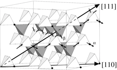
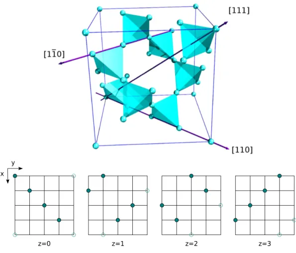
Competing magnetic interaction cause frustration and may prevent conventional magnetic order. As a consequence, complex ground states with unusual excitations can be realized, leading to a variety of interesting physical properties. One example is the so-called spin-ice material Dy2Ti2O7. In Dy2Ti2O7, the magnetic Dy ions form a pyrochlore sublattice, consisting of corner-sharing tetrahedra.

Due to a strong crystal field, the Dy momenta are aligned along their local easy axes pointing either into or out of the tetrahedra. The magnetic Dy ions inter- act via nearest-neighbor exchange and long-range dipole-dipole interaction. This highly frustrated spin-spin interaction is analogous to the proton displacement in water ice and leads to a residual entropy given by the Pauling’s entropy [1].

The macroscopically degenerate spin-ice ground state is realized by the ice rule 2in-2out which is fulfilled when two Dy spins per tetrahedra point into and the other two out of the tetrahedra. Elementary dipole excitations can be created by flipping one spin resulting in two neighboring tetrahedra with configurations 3in-1out and 1in-3out, respectively. These dipole excitations can fractionalize into two individual monopole excitations which can move independently within the pyrochlore lattice and are realizations of Dirac monopoles which are connected via Dirac strings [2].

Less is known about the interaction of these monopole excitations with each other or with other quasi particles. The aim of this thesis is to investigate the dynamics of these monopole excitations. In Refs. [3, 4], the observation of a monopole current due to a small magnetic field was reported. This point, however, is currently under strong debate [5] and remains an open question up to now. Suitable probes to study the dynamics of such elementary excitations are measurements of the thermal conductivity which are the main subject of this thesis. Up to now, only one experimental study about the thermal conductivity of Dy2Ti2O7 is published [6]. This work focuses on the relaxation times of the magnetic system in Dy2Ti2O7 which are anomalously enhanced at lowest temperatures. In Ref. [6], the thermal conductivity has been measured along the [110] direction for magnetic fields up to 1.5 T parallel to the heat current ~j.

Within this thesis, the thermal conductivity of Dy2Ti2O7 has been measured in great detail for different heat-current directions and various magnetic-field directions.

To study the different transport mechanisms contributing to the heat transport, three reference compounds are investigated in this thesis, the non-magnetic Y2Ti2O7 and two doped magnetic reference compounds (Dy_0.5Y0.5)2Ti2O7

(10)

and Dy₂(Ti0.9Zr0.1)2O7. In case of (Dy_0.5Y0.5)2Ti2O7, the idea is to suppress the spin-ice features by essentially conserving the phononic properties. In Dy₂(Ti_0.9Zr_0.1)₂O₇, the substitution with much larger Zr ions is supposed to affect the phononic properties by basically conserving the spin-ice properties.

Unconventional magnetic ordering can also be observed when reducing the dimensionality of the magnetic system, i.e.in low-dimensional spin systems. The second part of this thesis concerns the quasi one-dimensional antiferromagnetic spin-chain compound BaCo2V2O8, which is a realization of an effective spin-1/2 Ising-like spin chain. For magnetic fields parallel to thecaxis, the magnetization saturates at Bs|| ≃ 23 T and perpendicular to the c axis at Bs⊥ ≃ 41 T. In zero field, the system orders due to inter-chain coupling at TN= 5.4 K [7].

In low-dimensional spin systems, magnetic excitations can lead to large and unusual magnetic heat transport [8]. In integrable spin models, the heat transport is ballistic, i.e. dissipationless, and the magnetic thermal conductivity diverges. Enhanced heat transport was found mainly for low-dimensional S = 1/2 Heisenberg spin systems, like spin chains, spin ladders, and 2D square lattices. In this context, the question arises whether a magnetic heat transport can be observed for the Ising-like spin chain BaCo2V2O8. To resolve this issue, the thermal conductivity of BaCo2V2O8 has been measured for different heat- current directions parallel and perpendicular to the spin chains and for various magnetic-field directions. To study the transport mechanisms in BaCo2V2O8, additional thermal-conductivity measurements have been performed on two doped compounds, (Ba0.9Sr0.1)Co2V2O8 and Ba(Co0.95Mg_0.05)2V2O8, and on the iso-structural BaMn₂V₂O₈. The idea of Sr doping in (Ba_0.9Sr_0.1)Co₂V₂O₈ is to increase defect scattering in order to suppress the phononic thermal conductivity by essentially conserving the magnetic properties. In Ba(Co0.95Mg_0.05)2V2O8, doping with the non-magnetic Mg splits the Co chains into finite chain segments.

This is assumed to have a strong influence on the magnetic system. The Heisen- berg S = 5/2 spin chain BaMn2V2O8 is an iso-structural reference compound with isotropic magnetic properties.

This thesis is structured as follows. First, a brief introduction into the theoretical and experimental framework of the thermal conductivity is given. In Sec. 4, the thermal-transport properties of the spin-ice compound Dy₂Ti₂O₇ is studied. Sec. 5 deals with the study of the thermal conductivity of the spin-chain compound BaCo2V2O8. In the appendix, additional measurements which were performed during this thesis are presented.

(11)

2 Theory

2.1 Thermal Conductivity

In this chapter, basics of transport theory are briefly summarized. A more detailed introduction can be found in Refs. [9–21]. The thermal conductivity κ of a solid is defined as

~j =−κ ~∇T , (2.1)

where~j is the heat current and∇~T is the temperature gradient over the sample.

The negative sign reflects the fact that the heat flows from the hot to the cold end of the sample. Generally, κ is a 2nd-order tensor. For an isotropic crystal, κ is reduced to a scalar κ. By means of the kinetic gas theory, the thermal conductivity κ can be written as

κ= 1

dcvℓ , (2.2)

where d is the dimensionality (usually d = 3) and c is the specific heat of the considered (quasi-) particles with mean velocity v and mean free path ℓ. In the case of phonons, the thermal conductivity is described by the Debye model, presented in the following chapters.

2.1.1 Phononic Contribution (Debye Model)

The phononic specific heat (lattice contribution) can be calculated via the Debye formula

c_ph= 9N_Ak_B T

ΘD

3Z Θ_D/T

0

x⁴e^x

(e^x−1)² dx , (2.3) where ΘD denotes the Debye temperature. The integral in Eq. (2.3) can only be numerically calculated. In the limitT → ∞, the integral converges to ¹₃(ΘD/T)³ and, thus, one obtains the high-temperature limit c = 3NAkB (Dulong-Petit).

ForT → 0, the integral in Eq. (2.3) converges to R_∞

0 = 4π⁴/15≈25.9758. This yields the low-temperature T³ dependence for the phononic specific heat

c_ph = 12π⁴ 5

N_Ak_B

ΘD3 T³. (2.4)

Within the Debye model, the phononic thermal conductivity is given by κph = kB

2π²v kB

~

3Z Θ_D/T

0

x⁴e^xτ(ω, T)

(e^x−1)² dx , (2.5)

(12)

where v is the mean sound velocity, ω is the phononic angular frequency, x= (~ω)/(kBT), and τ⁻¹(ω, T) =v/ℓ is the total scattering rate, where ℓ is the mean free path. The mean sound velocity can be estimated via

v = Θ_D kB

~

(6π²n)⁻^1/3, (2.6)

where n=N/V is the atomic density per volume.

The integrals in Eqs. (2.3) and (2.5) can only be numerically calculated. In this thesis, the calculations and the fitting of experimental data is performed by the numerical computation software Scilab [22]. Assuming the different scattering processes to act independently, the total scattering rate is given by the sum of the scattering rates of each process (Matthiessen’s rule), i.e.

τ_tot⁻¹ =X

i

τ_i⁻¹. (2.7)

A variety of different scattering rates can be found in literature. The scattering rates used for the analysis in this thesis are the following:¹

Boundary Scattering

τ_bd⁻¹ =v/L (2.8)

This term describes reflection of phonons by the crystal surface, where L is the characteristic sample length. At very low temperatures (T → 0), the phononic thermal conductivity is essentially dominated by boundary scattering, i.e. the mean free path is only limited by the effective sample length (ℓ∼L).

The phononic specific heat cph and the sound velocity can be estimated by Eqs. (2.4) and (2.6), respectively. By inserting these quantities into Eq. (2.2), one can estimate the phononic thermal conductivity at low temperatures (T → 0).

In Refs. [26, 27], this estimation of the phononic thermal conductivity at lowest temperatures is used to investigate the presence of phonon scattering on magnetic excitations in the low-temperature limit. The authors calculate the mean free path ℓ via Eqs. (2.2), (2.4), and (2.6) and compare the (temperature-dependent) mean free path ℓ with the effective sample width W = 2 ¯w/√

π, where ¯w is the geometric mean width of a rectangular sample [28–30]. For a ratioW/ℓ≃1, one can assume the phononic thermal conductivity to be affected only by boundary scattering. W/ℓ <1 indicates an additional scattering process, e.g. on magnetic excitations.

1A detailed discussion of different scattering rates can be found in Refs. [12, 17, 23–25].

(13)

Point-Defect Scattering

τ_pd⁻¹ =P ω⁴ (2.9)

This term describes scattering of phonons on point defects, where P is an adjustable parameter. Short-wave phonons are more scattered than long-wave phonons, which dominate at low temperatures. Thus, this term is most effective in the temperature range of the phononic maximum of κ(T). At higher temperatures, the Umklapp scattering dominates.

Umklapp Scattering

τ_um⁻¹ =Uω²T exp

−ΘD

uT

(2.10) This term describes Umklapp scattering, whereU and u are adjustable parame- ters. The parameteru reflects the temperature range where Umklapp scattering sets in.

Resonant Phonon Scattering

τ_res⁻¹ =R 4ω⁴∆⁴

(∆² −ω²)² (N0+N1) (2.11) This term describes resonant scattering on a two- (or multi-) level system [31, 32].

R is an adjustable parameter, ∆ is the energy splitting, and N0 and N1 are the population factors of the two considered levels. In the special case of a two- level system, N0 and N1 sum up to 1. This scattering process affects phonons with an energy (frequency) close to the energy splitting ∆, which can depend on temperature as well as on the external magnetic field.

Scattering on magnetic Excitations at a magnetic Transition

τ_mag⁻¹ =Mω⁴T²Cmag(T) (2.12) This term describes scattering on magnetic excitations around a magnetic transition [24, 25] and results in a suppression ofκ(T) around the transition temperature. M is an adjustable parameter andCmag(T) is the temperature-dependent magnetic specific heat, which exhibits a peak around the magnetic transition.

(14)

2.1.2 Minimum Thermal Conductivity

In the high-temperature regime, the phononic thermal conductivity is proportional to 1/T (due to Umklapp scattering). To avoid the mean free path ℓ to become smaller than the inter-atomic distance, one can introduce a minimum mean free path ℓmin [33, 34] and, thus, a lower limit for the relaxation times

τ(ω, T) = max

τ_Σ(ω, T),ℓmin

v

, (2.13)

whereτ_Σ(ω, T) is the relaxation time obtained from the scattering rates discussed above. The minimum mean free path results in a minimum thermal conductivity κmin at high temperatures (typically at room temperature).

2.1.3 Electronic Contribution

The transport properties of electrons are described in detail in Ref. [35]. Here, a brief introduction is given. The electronic contributionκel of the thermal conductivity can be obtained by Eq. (2.2). The specific heat of the Fermi gas is given by [10]

cel = 1 2π²nkB

T TF

(2.14) with the Fermi temperature TF =ǫF/kB and the electron density n. The Fermi energy can be expressed in terms of the Fermi velocity

ǫF = 1

2mv²_F. (2.15)

By inserting Eq. (2.14) into Eq. (2.2) one obtains κel= 1

3celvFℓ= π²nk²_BT τ

3m , (2.16)

where the dimensionality isd= 3 and the mean free pathℓ =vFτ can be written in terms of the scattering time τ. The electron mass is m = 9.1094·10⁻³¹kg [36]. Analogues to Eq. (2.2), the total scattering rate is the sum of the different scattering rates of each involved process,

τ_el⁻¹ =τ_defect⁻¹ +τ_el-ph⁻¹ . (2.17) At very low temperatures, the defect scattering dominates. As the defects are essentially temperature independent, the scattering rate is basically constant and results in a linear increase of the electronic thermal conductivity at very low temperatures. At higher temperatures, the scattering of electrons on phonons is the dominant process. This leads to a reduction ofκat higher temperatures and, thus, to a characteristic low-temperature maximum of κ(T) [37].

(15)

2.1.4 Wiedemann-Franz Law

Good electrical conductors (metals) also are good thermal conductors. This results from the fact that the electrons which carry the electric charge can also transport heat. Within the Drude model, the electrical conductivity is given by [11]

σ = ne²τ

m , (2.18)

wheren is the electron density, e= 1.602·10⁻¹⁹C is the elementary charge [36], τ is the scattering time, and m is the electron mass. Assuming only elastic scattering of the electrons, one obtains the Wiedemann-Franz law by combining Eqs. (2.16) and (2.18),

κel

σ = π² 3

kB

e 2

T ≡L0T , (2.19)

where L0 = 2.45·10⁻⁸WΩ/K² is the Lorenz number. In good metals, the electronic contributionκel is much larger than the phononic contributionκph, which can basically be neglected.

2.1.5 Magnetic Contribution

The preceding sections dealt with the heat transport by phonons and electrons.

In principle, every (quasi) particle with a specific heat and a non-vanishing group velocity can carry heat. A detailed introduction to the heat transport by magnetic excitations can be found in Refs. [8, 9, 38]. Here, the essential points of Ref. [8]

are briefly summarized.

Magnetic heat transport has been observed for a wide range of different mate- rials [39–45]. Here, we focus on a special class of magnetic systems with reduced dimensionality, i.e. one- or two-dimensional spin systems, and antiferromagnetic Heisenberg exchange between nearest-neighbor spins. The most prominent compounds realizing a magnetic heat transport are copper-oxide systems (cuprates) which will be introduced in the following.

Fig. 2.1 illustrates three different spin structures which are realized by various cuprate systems. S = 1/2 Heisenberg AF spin chains (Fig. 2.1(a)) are realized by, e.g., CaCu2O3, SrCuO2, and Sr2CuO3. The S = 1/2 Heisenberg AF two- leg spin ladder (Fig. 2.1(b)) can be realized by different compounds of the type (Sr,Ca,La)14Cu24O41. The 2D square lattice (Fig. 2.1(c)) can be regarded as a spin ladder with an infinite number of legs and can be realized by La2CuO4. These compounds have rather large coupling constants of J ≈1500 K− 2000 K [8].

The different spin structures shown in Fig. 2.1 have different ground-state properties and elementary excitations. Within the spin chain, the correlation of the spins is quasi-long range and decays algebraically with increasing distance

(16)

Figure 2.1: Different spin structures of antiferromagnetically coupled S= 1/2 Heisenberg spins. a) spin chain, b) two-leg spin ladder, c) two- dimensional square lattice (taken from [8]).

between the spins [46]. The elementary excitations are called spinons. They are gapless and carry a spin ofS = 1/2 [47]. The ground state of the two-legS = 1/2 Heisenberg spin ladder is a spin liquid. The short-range spin-spin correlations decay exponentially with increasing distances. The elementary excitations are magnons (triplons) with spin S = 1 and a spin gap ∆ [48]. The ground state of the antiferromagnetic Heisenberg S = 1/2 2D square lattice is a N´eel state [49].

The elementary excitations are spin waves.

The magnetic heat transport in one-dimensional antiferromagnetic S = 1/2 Heisenberg chains is predicted to be dissipationless, i.e. to have no thermal resis- tivity [50, 51]. This so-called ballistic heat transport originates from the fact that the thermal-current operator and the Hamiltonian commute, i.e. the thermal- current operator is a conserved quantity. The question whether the heat transport is conserved also in spin-ladder compounds is currently under debate [52–55]. In real crystals, the thermal conductivity is affected by external scattering processes and, hence, remains finite. In the following, experimental results of thermal- conductivity measurements are shown for different types of low-dimensional spin systems.

The upper panels of Fig. 2.2 illustrate experimental thermal-conductivity data for the compounds realizing the different spin structures shown in Fig. 2.1, i.e.

(a) spin chain, (b) spin ladder, and (c) 2D square lattice [8, 56–59]. The extracted magnetic contributions κmag are shown in the lower panels.² The magnetic thermal conductivityκmag of the gapless spin-chain compound CaCu2O3 (Fig. 2.2(a)) almost linearly increases with increasing temperature. The magnetic contribu- tionsκmagof the gapped spin-ladder compounds Sr14Cu24O41and Ca9La5Cu24O41

(Fig. 2.2(b)) show an activated behavior at low temperatures. At ∼150 K, depending on the actual compound, κmag exhibits a broad maximum and decreases

2Details of how to extract the magnetic contribution of the respect data can be found in [8].

(17)

Figure 2.2: Upper panels: Thermal conductivity of S= 1/2 Heisenberg antiferromagnets. (a) spin chain, (b) spin ladder, (c) 2D square lattice. Lower panels: Extracted magnetic thermal conductivity κ_mag for the respective spin systems (taken from [8, 56–59]).

at higher temperatures. Fig. 2.2(c) showsκmagfor the 2D square lattice La2CuO4. At low temperatures, κmag increases quadratically with increasing temperature and shows a maximum around∼300 K.

The spin systems presented up to here have rather large exchange couplingsJ.

In the following, a class of low-dimensional spin systems with much lower exchange energies is presented. Due to the lower J, one can strongly influence the spin gap by magnetic fields which can be realized by typical laboratory mag- nets. A disadvantage of the lower J, however, is that one needs to measure the thermal conductivity at far lower temperatures well below 1 K to observe κmag. A magnetic heat transport was observed for the Haldane spin-chain compound Ni(C2H8N2)2NO2(ClO4) (NENP) [60] and for the S= 1/2 Heisenberg spin-chain compound Cu(C4H4N2)(NO3)2 (CuPzN) [61, 62]. The latter will be briefly discussed in the following.

CuPzN is a HeisenbergS= 1/2 spin chain with intra-chain exchange coupling J = 10.3 K and a rather small inter-chain coupling|J^′/J| ≈4·10⁻³ [63–65]. At a critical fieldBc= 15.0 T, the spin system enters a gapped phase. The reduction of κ(B) parallel to the spin chains due to the magnetic field is illustrated in

(18)

Figure 2.3: Magnetic-field dependent reduction ofκ(B) for CuPzN at various constant temperatures between 0.37 K and 7.82 K (taken from [61]).

Fig. 2.3. At lowest temperatures, κ(B) stays almost constant up to ∼13 T. At higher fields, κ(B) decreases with increasing field and forms a plateau around the critical fieldB_c. For fields aboveB_c,κ(B) further decreases. The plateau feature is observable up to ∼2.5 K, although broadened. Above ∼3.5 K, the plateau feature vanishes. At low temperatures and small magnetic fields, κ(B) exhibits a small local minimum which can probably be attributed to phonon scattering on magnetic excitations (cf. discussions in Ref. [66]).

The thermal-conductivity data in Fig. 2.3 very clearly show the presence of a magnetic heat transport within the gapless phase below Bc. AboveBcwhere the spin gap opens, κ(B) drastically decreases with increasing field. The magnetic thermal conductivity κmag can be calculated via mean-field theory including the Jordan-Wigner transformation [67–69] by assuming a momentum-independent mean free pathℓ. Comparison with experimental data provide an essentially field- independent mean free path which increases linearly with increasing temperature [61]. This is in accordance to theoretical predictions for Luttinger liquids [61, 70, 71].

Heisenberg Spin-ladder compounds with rather small exchange couplings can be realized by (C₅H12N)₂CuBr4 (HPIP) and (C₇H10N)₂CuBr4 (DIMPY). The main difference between HPIP and DIMPY is the ratio of the exchange couplings along the legs and the rungs, J_|| and J_⊥, respectively. In the case of HPIP, the coupling J_|| ≃3.6 K is smaller than J_⊥ ≃13 K [66, 72–78]. Between the critical fieldsBc₁ ≃6.6 T andBc₂ ≃14.6 T [72], the zero-field spin gap ∆≃9.5 K vanishes and the spin system is in a Luttinger-liquid state. In the case of DIMPY,

(19)

the leg couplingJ_|| ≃8.4 K is larger than the rung couplingJ_⊥≃4.3 K. The spin system has a zero-field spin gap of ∆≃3.7 K and two critical fields Bc1 ≃3 T and B_c₂ ≃30 T [79, 80].

The thermal conductivity of HPIP has been measured in magnetic fields up to 17 T at temperatures down to 0.37 K [66]. In this temperature range, no magnetic heat transport is observed, i.e. κ is purely phononic. The field dependence of κ can be attributed to scattering on magnetic excitations in the gapless phase [66].

Up to now, no literature data of the thermal conductivity of DIMPY has been published.

Within the framework of this thesis, efforts were made to measure the thermal conductivity of HPIP and DIMPY in a dilution refrigerator, to test if a magnetic contribution κmag is observable at lower temperatures. Due to weak thermal couplings of the HPIP crystals to the sample holder, the κ measurements were only possible above 0.2 K. The results are shown in Appendix A (Fig. A.1).

The features observed in κ(B) above 0.4 K [66] can be reproduced up to 10 T.

When lowering the temperature, the observed features indeed become sharper.

However, no magnetic heat transport can be observed down to 0.2 K.

The thermal conductivity of DIMPY has been measured down to 0.35 K.

Due to sample instability and incompatibility with the adhesives, the thermal conductivity could not be measured reproducibly. Two datasets of κ of DIMPY are shown in Appendix A (Figs. A.4 and A.5). Unfortunately, both datasets show a different behavior and do not allow a conclusive interpretation. Hence, the question whether the spin-ladder compound DIMPY shows magnetic heat transport remains an open question.

2.2 Demagnetization

The demagnetization field (stray field) is a magnetic field which is generated by the magnetization M of a magnetic sample. In case of a paramagnet, the demagnetization field counteracts an external magnetic fieldHext and, thus, leads to a reduction of Hext. As the magnetization M(H) itself is a response to an external magnetic field, magnetization and demagnetization influence each other.

In case of a paramagnet, an increase of the external field leads to an increase of the magnetization and, thus, to a reduction of the causative field.

The demagnetization effect is strongly anisotropic with respect to the sample geometry and to the sample orientation within the external magnetic field (shape anisotropy). For the simplified case of an ellipsoidal sample, the demagnetization fieldHDis homogeneous within the sample and proportional to the magnetization M, i.e.

HD=−DM , (2.20)

whereD is the demagnetization factor which depends on the actual shape of the

(20)

0.0 0.2 0.4 0.6 0.8 1.0 0.0

0.2 0.4 0.6 0.8 1.0

(a)

c/b = 1 c/b = 0.5

c/b = 0.25 c

b

D

1.25 1.67 2.5 5 ∞

B

a

a = c

c/b

c/b = 2 c/b = 4 a = b

B

0.0 0.2 0.4 0.6 0.8 1.0

(b)

c/b = 1

c/b = 0.5 c/b = 0.25

c b

D

1.25 1.67 2.5 5 ∞

B

a

a = b

c/b

c/b = 2

c/b = 4 a = c

B

Figure 2.4: Demagnetization factor of a (a) cigar and (b) planar-shaped ellipsoidal sample as a function of the ratios of the semi-major axes a,b, and c. The external magnetic field is directed parallel to b. [81]

ellipsoid. Hence, the reduced magnetic field is given by

H =Hext−DM . (2.21)

Obviously, the demagnetization field HD becomes constant when the magnetization reaches its saturation value. For larger fields, the demagnetization correction simply is a constant offset.

The demagnetization factor D of an ellipsoid can be calculated numerically depending on the ratio of the three semi-major axes a, b, and c [81]. Fig. 2.4 shows the demagnetization factor D for a cigar- and a planar-shaped ellipsoidal sample (panel (a) and (b), respectively). In both cases, the special case of a circle (a = b = c) leads to a demagnetization factor of D = 1/3. On the left

(21)

hand side of Fig. 2.4(a), the magnetic field is parallel to the long semi-major axis b. For an infinitesimally thin sample, the demagnetization factor vanishes.

On the right hand side, the magnetic field is directed along one of the short axes.

Here,Dconverges to 1/2 for an infinitesimally thin sample. Fig. 2.4(b) shows the demagnetization factor of a planar-shaped sample. When applying the magnetic field parallel to one of the longer semi-major axes, D vanishes in the limit of an infinitesimally thin plane. ForB~ parallel to the short axis, the demagnetization factor converges to 1 in the limit of an infinitesimally thin plane.

Demagnetization effects can be minimized by choosing a suitable sample geometry, i.e. a thin planar- or cigar-shaped sample with the long edge parallel to the external magnetic field. In some cases, the measurement setup inhibits a convenient orientation of the sample with respect to the magnetic field. In this case, the demagnetization can have a strong influence on the applied external field. Therefore, the demagnetization field has to be subtracted from the external field to obtain the correct internal field. This requires the knowledge of the actual magnetization M(H), which has to be measured separately on a sample of suitable shape.

One possibility to calculate HD is to approximate the sample by an ellipsoid with a known demagnetization factor. Alternatively, one can calculate the demagnetization field numerically by means of a Mathematica script (written by O. Breunig), which makes use of the Radia package [82, 83]. The script works as follows. The spatial distribution of the magnetic field inside the sample is calculated on the basis of experimental magnetization data. Generally, one can choose an arbitrary sample geometry within the calculation software. The demagnetization corrections for the measurements within the framework of this thesis were done by approximating the samples as rectangular-shaped samples.

In a last step, the average internal magnetic field is obtained by integrating the field over the whole sample.

The thermal-conductivity measurements are treated in a slightly different way.

As one can make an assertion about the measured κ only between the different temperature contacts (Fig. 3.1 on page 24), which are attached on the sample at approximately 1/3 and 2/3 of the sample height, the average magnetic field is obtained by integrating over the sample volume between these two temperature contacts.

All measurements within this thesis, including a magnetic field, were corrected by means of this script. The corresponding magnetization data were measured by M. Hiertz during his diploma thesis [84].

(22)

(23)

3 Experimental

This chapter concerns the experimental environment and the measurement techniques used to obtain the data presented in this thesis. The main focus lies on the thermal-conductivity measurements, which will be described in detail.

The magnetization and magnetostriction measurements were performed by M. Hiertz during his diploma thesis [84] and will be described in detail there.

The magnetization measurements were done with a home-built force magnetome- ter which has been built up by D. Loewen and further modified by S. Scharffe during their diploma theses [85, 86]. The magnetostriction measurements were performed with a home-built capacitance dilatometer which has been built by O. Heyer during his diploma thesis [87]. The principle ideas of the capacitance dilatometry are described in Ref. [88].

3.1 Thermal-Conductivity Measurements

The thermal conductivityκcan be measured via the steady-state method, which will be explained in the following. In one dimension, the definition of κ (Eq. 2.1 on page 11) can be rewritten into the form

P

A =κ∆T

∆x . (3.1)

The heat currentj =P/Ais given by the ratio of the sample-heater powerP and the sample cross sectionA. The temperature gradient ∆T /∆xis assumed to be constant within the sample. Therefore, one needs to measure the temperature difference ∆T between two determined levels of the sample with distance ∆x.

To ensure a homogeneous heat current within the sample, one needs to chose a suitable sample geometry. The sample should be a thin crystal with the long edge parallel to the heat current.

Fig. 3.1 illustrates the steady-state method to measure the thermal conductivity. In order to measure κ via Eq. (3.1), one needs to know the geometry of the sample, i.e. Aand ∆x, the heating powerP, and the temperature difference

∆T. The heating power is the product of the heater current IH and the voltage dropUHover the heater. The temperature difference ∆T can be measured by two different approaches. One can either measure ∆T via a thermocouple or one can measure the absolute values of the temperatures at both levels. The technique including the thermocouple is used in the temperature range between 5 K and 300 K. The method including two thermometers can be used below ∼20 K, in

(24)

Figure 3.1: Steady-state method to measure the thermal conductivity. The temperature gradient is produced by a sample heater on top of the sample.

The temperature difference can either be obtained via a thermocouple or via two thermometers attached at the sample.

principle, down to lowest temperatures. Both techniques will be described in the following.

3.2 Thermal-Conductivity Measurements in the High- Temperature Regime

In the temperature range between 5 K and 300 K, the temperature difference is measured via a thermocouple as shown in Fig. 3.2. The advantage of this measurement technique is that one directly measures the temperature difference

∆T. As a drawback, one cannot directly measure the actual sample temperature as the thermometer is placed on the sample-holder platform. Heating the top of the sample certainly heats up the whole sample. In this temperature regime, the thermal resistance between sample and sample holder usually is rather small, compared to the low-temperature region discussed below. One possibility to directly measure such a heating is to use a second thermocouple which measures the temperature difference between the sample-holder thermometer and the lower end of the primary thermocouple.

The thermocouple used here consists of Chromel³ and a gold-iron alloy (0.07% iron). This sort of thermocouple has been used within many diploma and PhD theses. The thermocouples used in this thesis are made of one peace of gold (0.07% iron) wire (∼10 cm) and two Chromel wires (∼5 cm). Both wire types

3Chromel consists of 90% nickel and 10% chromium.

(25)

Figure 3.2: Photograph of a thermocouple consisting of chromel and a gold- iron alloy (0.07% iron).

0 50 100 150 200 250 300

10 12 14 16 18 20 22

0 T 4 T 8 T 12 T

S (µV/K)

T (K)

0 10 20 30

10 12 14 16 18 20

S (µV/K)

T (K)

Figure 3.3: Thermopower of the thermocouple used here for various constant magnetic fields. This inset schematically shows the experimental setup used to calibrate the thermocouple.

(26)

have a rubber-like cable insulation, which has to be removed at both ends. This can be done with a scalpel. The Chromel wire is rather robust. The gold wire, however, has to be treated very cautiously. Another difficulty is to solder up the ends of the respective wires. To be able to solder the Chromel wire, first, it has be treated with an acid flux. The major problem, however, is to solder the gold wire as it melts quickly at a rather low temperature. This can be best done with solder tin containing lead. This reduces the melting point to ∼180^◦C.

The thermocouple has been calibrated for various magnetic fields. The results are shown in Fig. 3.3 for zero field and for three different magnetic fields.

Below 60 K, the thermopower strongly depends on the magnetic field. In this temperature region, the thermopower S(T) has been measured for 0 T, 2 T, 4 T, 6 T, 8 T, 10 T, 12 T, 14 T, and 16 T. Above 60 K, the thermopower is hardly field dependent. Here, the S(T) curves are measured in 0 T, 6 T, and 14 T.

The experimental setup to calibrate the thermocouple is schematically illustrated in the inset of Fig. 3.3. It is similar to the calibration setups presented in e.g. Refs. [31, 89]. Both ends of the thermocouple are attached at the sample- holder platform and on a sapphire plate with temperaturesT0andT1, respectively.

The sapphire plate is thermally decoupled from the sample-holder platform via a thick Manganin⁴ wire. The temperature difference ∆T = T1−T0 is produced by a heater placed on the sapphire plate.

3.3 Thermal-Conductivity Measurements in the Low- Temperature Regime

Below 5 K, the thermopower of the thermocouple used here rapidly vanishes (see Fig. 3.3). Therefore, one has to measure the temperature difference via two individual thermometers, i.e. ∆T = T2−T1. The advantage of this method is the knowledge of the absolute temperatures T₁ and T₂ directly at the sample.

Therefore, one can determine the actual sample temperature as the mean value of both temperatures, i.e. Tsample = ¹₂(T1 + T2). This is very important as the thermal-contact resistances between the sample holder and the sample often become very large at lowest temperatures.

The challenge is to accurately calibrate both thermometers at the sample.

A reasonable temperature difference should be in the order of several percents of the sample temperature. Thus, both thermometers have to provide the same absolute values within a tolerance well below 1 per mill. Therefore, both thermometers have to be calibrated within each measurement run as every cooling of the thermometers leads to a slight change of the R(T) characteristics. A detailed description of the techniques to measure the temperature is given in Sec. 3.5.

The thermometers are calibrated with respect to the sample-holder thermometer. It is important to calibrate both thermometers simultaneously to ensure that

4Manganin consists of copper (86%), manganese (12%), and nickel (2%) [90].