Thermodynamics and Heat Transport of doped Spin-Ice Materials

Thermodynamics and Heat Transport of doped Spin-Ice Materials

I n a u g u r a l - D i s s e r t a t i o n

zur

Erlangung des Doktorgrades

der Mathematisch-Naturwissenschaftlichen Fakult¨ at der Universit¨ at zu K¨ oln

vorgelegt von

Simon Scharffe

aus Bergisch Gladbach

K¨ oln, 2016

Vorsitzender der Pr¨ ufungskommission: Prof. Dr. S. Trebst

Tag der m¨ undlichen Pr¨ ufung: 22.04.2016

Contents

1 Introduction 1

2 Theory 5

2.1 Specific heat . . . . 5

2.1.1 Phonon contribution . . . . 6

2.1.2 Electronic contribution . . . . 7

2.1.3 Schottky anomaly . . . . 7

2.2 Thermal conductivity . . . . 8

2.2.1 Phonon contribution . . . . 9

2.2.2 Electron contribution . . . . 10

2.2.3 Heat transport by magnetic excitations . . . . 10

2.3 Demagnetization . . . . 11

3 Experimental 13 3.1 Cryogenic environments . . . . 13

3.2 Magnetization . . . . 15

3.3 Thermal conductivity . . . . 16

3.3.1 Low-temperature sample wiring . . . . 17

3.3.2 Calibration of RuO ₂ thermometers . . . . 19

3.3.3 Measurement instruments . . . . 20

3.4 Thermal expansion and magnetostriction . . . . 21

3.5 Specific heat . . . . 22

3.5.1 Relaxation method . . . . 22

3.5.2 Heat-flow method . . . . 24

3.6 Magnetocaloric effect . . . . 27

4 Introduction to spin ice 33 4.1 Magnetic frustration . . . . 33

4.2 History . . . . 34

4.3 Single-tetrahedron approximation in external magnetic field . . . . 40

4.4 Internal thermal equilibration . . . . 43

4.5 Pauling’s residual entropy . . . . 44

4.6 Magnetic monopoles & dumbbell model . . . . 46

4.7 Monopole dynamics . . . . 49

4.8 Literature heat transport . . . . 50

5 Sample characterization 55

5.1 Crystal growth . . . . 55

5.2 Dilute spin ice: (Dy _1-x Y _x ) ₂ Ti ₂ O ₇ . . . . 56

5.2.1 Literature . . . . 56

5.2.2 Magnetization . . . . 58

5.3 Zirconium doping: Dy ₂ (Ti _1-x Zr _x ) ₂ O ₇ . . . . 59

5.4 Dilute spin ice: (Ho _1-x Y _x ) ₂ Ti ₂ O ₇ . . . . 61

5.4.1 Literature . . . . 61

5.4.2 Magnetization . . . . 62

5.5 Zirconium doping: Ho ₂ (Ti _1-x Zr _x ) ₂ O ₇ . . . . 63

6 Ho

Ti

O

vs. Dy

Ti

O

65 6.1 Literature results . . . . 65

6.2 Experimental results . . . . 66

6.2.1 Magnetic field || [001] . . . . 66

6.2.2 Magnetic contribution . . . . 75

6.2.3 Magnetic field || [111] . . . . 78

6.3 Conclusion . . . . 82

7 Dilute spin ice (Dy

Y

)

Ti

O

83 7.1 Hysteresis and relaxation effects . . . . 83

7.1.1 H ~ || [001] and ~ j || [1¯ 10] . . . . 84

7.1.2 H ~ || [111] and ~ j || [1¯ 10] . . . . 86

7.1.3 H ~ || [111] and ~ j || [111] . . . . 89

7.1.4 Conclusion . . . . 94

7.2 Specific heat and entropy . . . . 95

7.2.1 Literature results . . . . 95

7.2.2 Experimental results . . . . 97

7.2.3 Conclusion . . . 111

7.3 Heat transport . . . 111

7.3.1 Literature results . . . 111

7.3.2 Experimental results . . . 114

7.3.3 Conclusion . . . 125

8 Summary 127 A 1D Ising-chain system CoNb

O

131 A.1 Introduction . . . 131

A.1.1 Crystal structure . . . 131

A.1.2 Sample growth . . . 132

A.1.3 Literature results . . . 133

Contents

A.2 Experimental results . . . 133

A.2.1 Magnetization . . . 133

A.2.2 Specific heat . . . 136

A.2.3 Phase diagram . . . 139

A.3 Comparison to 1D Ising model in transverse magnetic field . . . 142

A.4 Quantum criticality . . . 145

A.5 Conclusion . . . 146

Bibliography 149

List of Figures 161

List of Tables 165

Publikationsliste 167

Danksagung 169

Zusammenfassung 171

Abstract 173

Offizielle Erkl¨ arung 175

1 Introduction

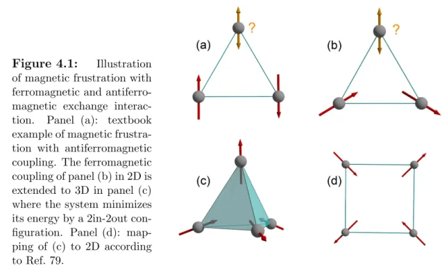
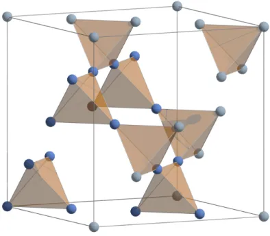
In the field of condensed-matter physics the concept of magnetic frustration leads to fascinating properties which arise from microscopic details of the interplay between different interactions and geometric constraints leading to the existence of complex ground states and exotic excitations [1–3]. Among these exotic excitations are frac- tionalized electric charges in the quantum Hall effect and fractionalized magnetic dipoles in a class of geometrically frustrated magnets known as spin ice [4]. Pro- totype spin-ice materials are the pyrochlores Dy ₂ Ti ₂ O ₇ and Ho ₂ Ti ₂ O ₇ where the geometric frustration of magnetic interactions prevents long-range magnetic order down to lowest temperature. The magnetism of both materials can be well de- scribed by non-collinear S = 1/2 Ising spins with large magnetic moments of about µ = 10µ _B that form a network of corner-sharing tetrahedra. A strong crystal elec- tric field results in an Ising anisotropy with quantization axes pointing along the lo- cal {111} directions. Antiferromagnetic nearest-neighbor exchange interactions are overcome by strong dipolar interactions leading to an effective ferromagnetic cou- pling. A sixfold degenerate ground state with two spins pointing into and two out of each tetrahedron originates from the interplay between the geometric constraints and the effective ferromagnetic coupling. This 2in-2out arrangement is equivalent to Pauling’s ice rule describing the hydrogen displacement in water ice and results in a residual zero-temperature entropy of S _P = R/2 ln(3/2) [5, 6]. The lowest excitation in spin-ice systems is a single spin flip which creates a pair of 1in-3out and 3in-1out configurations on neighboring tetrahedra and due to the ground-state degeneracy such a pair can fractionalize into two individual excitations that can propagate almost independently within the pyrochlore lattice. These unique excitations are described as (anti-)monopoles connected via Dirac strings [4, 7].

The knowledge about the dynamics of these monopoles and their interaction with

phonons is still limited [8–10]. A suitable method to investigate the dynamics of the

monopoles are measurements of the thermal conductivity. However, a possible mon-

opole contribution to the heat transport is under strong debate [11–15]. Refs. 11–13

assume a phonon-dominated heat transport in zero field and a field-induced suppres-

sion of κ _ph by some field-dependent scattering mechanisms of phonons by magnetic

excitations. Ref. 13 attributes a low-field decrease of κ(H) to a possible magnetic

contribution but the description within the Debye-H¨ uckel theory fails which is in-

terpreted to be a lack of evidence for monopole heat transport. In Refs. 14, 15,

the interpretation differs and is based on a comparative study of (Dy _1−x Y

) ₂ Ti ₂ O ₇ with x = 0, 0.5, and 1. It is found that, in the high-field range above about 1.5 T, a field-induced suppression of κ ph (H) is present for both, the spin ice Dy 2 Ti 2 O 7 and the highly dilute (Dy _0.5 Y _0.5 ) ₂ Ti ₂ O ₇ in which spin-ice behavior is essentially sup- pressed [16, 17]. In the pure Dy ₂ Ti ₂ O ₇ , however, an additional low-field decrease of κ(H) is observed. The anisotropic field dependence and the hysteresis behavior clearly correlate with the spin-ice physics. All these findings evidence a sizable κ _mag in zero field, which is successively suppressed by an external magnetic field due to the field-induced suppression of the monopole mobility. Experimental indication for a zero-field monopole contribution to the heat transport has also been proposed from an analysis of κ(T ) of Ho ₂ Ti ₂ O ₇ at different magnetic fields [18]. However, the magnitude of κ _mag estimated for Ho ₂ Ti ₂ O ₇ is more than an order of magni- tude smaller than κ _mag of Dy ₂ Ti ₂ O ₇ . To address the question if the monopoles contribute to the thermal conductivity of spin ice, in this thesis a detailed com- parative study of the different thermodynamic properties of Ho ₂ Ti ₂ O ₇ , Dy ₂ Ti ₂ O ₇ and the corresponding 50% dilute reference materials is performed to clarify the influence of magnetic excitations on the heat transport. The measurements are accomplished at temperatures ranging from 0.3 to 10 K and magnetic fields up to 7 T using custom setups. In addition, the thermal conductivity of the dilution se- ries (Dy _1−x Y

) ₂ Ti ₂ O ₇ for various x is obtained in order to get a more quantitative verification of the monopole contribution to the heat transport. A special emphasis is also put on the low-field hysteresis and relaxation phenomena observed in the thermal conductivity of Dy ₂ Ti ₂ O ₇ at lowest temperature. It is studied in how far equilibration states are realized.

The long-predicted residual entropy for spin ice [5, 6] has been expanded to a gen- eralized Pauling approximation for dilute spin ice [19] where the magnetic Dy ³⁺ or Ho ³⁺ ions are partly replaced by non-magnetic elements. This generalization has been demonstrated by first studies [19]. But recently, an absence of Pauling’s resid- ual entropy S _P in Dy ₂ Ti ₂ O ₇ has been reported based on measurements of the specific heat over timescales of 10 ⁴ s [20]. To address this discrepancy, the temperature- and field-dependent change of entropy of the dilution series (Dy _1−x Y

) ₂ Ti ₂ O ₇ with x = 0–0.75 is studied by means of the specific heat and the magnetocaloric effect in a temperature range from 0.3 to 30 K. Additional information about the low- temperature thermal equilibration of the systems is gained. Furthermore, Monte Carlo data on the magnetic specific heat and entropy of dilute spin ice have been published [21] which are quantitatively compared to the obtained experimental results.

This thesis is structured as follows. First, a brief overview of the theoretical and experimental work is given in Chap. 2 and 3. In Chap. 4, the spin-ice materials are introduced and the most important findings on these systems are summarized.

The sample characterization of the spin-ice compounds is presented in Chap. 5. A

comparative study of the spin-ice compounds Ho ₂ Ti ₂ O ₇ and Dy ₂ Ti ₂ O ₇ is performed

in Chap. 6 followed by a detailed study on the heat transport and specific heat of

dilute spin ice (Dy _1−x Y

) ₂ Ti 2 O 7 in Chap. 7 for different directions of the applied

magnetic field. A summary of this work is followed by the appendix where the study

on the quasi 1D Ising-chain system in transverse magnetic field of the diploma thesis

is continued by measurements of the magnetization.

2 Theory

This chapter gives an introduction into the basic concepts and models that are employed in the discussions of the spin-ice systems. A broad overview about con- ventional mechanisms established in literature is given, and some important basic relations are quoted. More detailed descriptions and further information can be found in literature [16, 22–36].

2.1 Specific heat

The specific heat is one of the fundamental thermodynamic properties. It can provide insights into excitations and phase transitions of solids, gases and fluids.

The molar specific heat at a constant volume V or pressure p is given by [24]

c

= N _A /N ∂U

∂T

c

= N _A /N ∂U

∂T

(2.1) with the number of particles N , the Avogadro constant N _A and the internal energy U . In a real experiment, it is very difficult to keep the volume of a solid constant and that is why c

is the experimentally accessible property. However, the relative difference between c

and c

is smaller than 1% in solids for T < 300 K. Thus, in most cases it is not differentiated between both properties. The total differential of the internal energy U = U (S, V, N ) of a system is

dU = T dS − p dV + µ dN (2.2)

with the entropy S, the temperature T , and the electrochemical potential µ. From Eq. (2.2), the relation between c

and the entropy S is given by

c

= N _A N

∂U

∂T

= N _A N T ∂S

∂T

. (2.3)

The entropy S is obtained by temperature integration via S = N A

N

T

Z

0

c

(T

)

T

dT

. (2.4)

The specific heat measures the sum of all thermal excitations of a system whereas a separation of the single contributions can be very difficult. However, elementary excitations like phonons or magnons show characteristic temperature dependencies that allow a distinction. The phononic contribution to the specific heat can be either estimated by models, e.g. the Debye model, or by measurements of non- magnetic reference materials.

2.1.1 Phonon contribution

The law of Dulong-Petit uses a classical Ansatz and yields a temperature- independent molar specific heat of

c

= f

2 N A k B (2.5)

where f are the degrees of freedom. Thus the molar specific heat is obtained via c

= 3N _A k _B = 3R with the general gas constant R = 8.31 J/mol K.

Quantum mechanical models are applied to calculate the specific heat in the low- temperature regime. The models invented by A. Einstein and P. Debye are based on the same ansatz. Both models use the Ansatz for the phonons to be harmonic oscillators whose internal energy can be derived via [37]

U = Z

D(ω)hn(ω)i ~ ωdω (2.6)

with density of states D(ω) and hn(ω)i as the thermal population value of a 1- dimensional oscillator with frequency ω.

Within the Debye model, an averaged isotropic linear dispersion relation ω = v _s k is assumed with the average sound velocity v _s . Then, the density of states in 3 dimensions is given by D(ω) = V ω ² /2π ² v _s ³ with the volume V of the solid. The molar specific heat is obtained via [24]

c _V = 9R T

Θ D

3

T ³

Z Θ

0

x ⁴ e

(e

− 1) ² dx (2.7)

with x = ( ~ ω) / (k _B T ) and the Debye temperature Θ _D . The integral in Eq. (2.7) can only be solved numerically and for low temperatures (T Θ _D ) the equation converges to the famous T ³ -dependence of the lattice contribution to the specific heat

c V = 12π ⁴ 5 R

T Θ _D

3

= βT ³ . (2.8)

2.1 Specific heat

For high temperatures (T Θ _D ), Eq. (2.7) yields the classical Dulong-Petit for- mula c _V = 3R.

In the low-temperature range (T Θ D ), the Debye model yields a good description of the phononic specific heat of solids. Here, the long-wavelength acoustic phonons are mostly populated which show a nearly linear dispersion. However, systems that reveal flat optical phonon branches are not well described [24, 37, 38]. These flat optical phonon branches (ω is almost constant) are often approximated by the Einstein model in which the phononic contribution is estimated by considering N oscillators with the same frequency ω. Thus, the internal energy from Eq. (2.6) is given by [24]

U = 3N hni ~ ω = 3N ~ ω

e

− 1 . (2.9)

The factor 3 accounts for the three degrees of freedom of every single oscillator. By applying Eq. (2.3), the specific heat is obtained via [24]

c

= ∂U

∂T

V

= 3N _A k _B ~ ω

k _B T 2

e

e

− 1 . (2.10) In the high-temperature limit, the Einstein model is also equivalent to the law of Dulong-Petit.

2.1.2 Electronic contribution

The electronic contribution to the specific heat can be obtained from considerations of the free electron gas in a solid. The molar specific heat of the free electron gas is given by

c el = Rπ ² 2

T

T _F = γT (2.11)

where T _F is the Fermi temperature. The total specific heat c _tot = c _ph + c _el in the low-temperature limit T Θ _D T _F is often expressed in terms of

c tot

T = γ + βT ² (2.12)

where β follows from Eq. (2.8).

2.1.3 Schottky anomaly

The Schottky anomaly is an effect which results from the thermal population of

higher-lying discrete energy levels. The internal energy U of N non-interacting

particles with energy levels E

with degeneracy g

is given by

U = N P

i

E

g

exp(−E

/k _B T )

Z . (2.13)

with the partition sum Z = P

i

g

exp(−E

/k B T ). The molar specific heat of a sys- tems of non-interacting particles with discrete energy levels follows from Eq. (2.13) by c = N _A /N

to be

c sch = N _A k _B T ²

P

i

E

² g

exp(−E

/k _B T )Z −

P

i

E

g

exp(−E

/k _B T ) 2

Z ² (2.14)

In the case of a two-level system, where the first g ₁ -fold degenerate excited state is separated from the g ₀ -fold degenerate ground state by the energy gap ∆E, Eq. (2.14) simplifies to

c 2,sch = N _A ∆E ² k _B T ²

g ₁ g ₀

exp(−∆E/k _B T )

1 +

0

exp(−∆E/k _B T ) 2 . (2.15)

2.2 Thermal conductivity

The thermal conductivity κ of a solid is given by

~j = −κ ~ ∇T (2.16)

with the heat current ~j and the temperature gradient ∇T ~ over the solid. The negative sign is related to the fact that the heat flows from the hot end to the cold end of the sample. In general, the thermal conductivity κ is a 2nd-order tensor which reduces to a scalar κ in an isotropic system.

If the kinetic gas theory is applied, the thermal conductivity is determined by heat carrying (quasi-)particles and it can be expressed via [24]

κ = 1

d cv` (2.17)

where d denotes the dimensionality, c the specific heat, v the group velocity and

` = vτ the mean free path of the heat carrying quasi-particles (τ is the relaxation time). In most cases two kinds of excitations are responsible for the heat transport:

phonons and electrons. The theoretical description is usually based on the Debye

model for phonons, and on electronic gas theory for the electrons.

2.2 Thermal conductivity

2.2.1 Phonon contribution

The heat carrying quasiparticles in an insulating crystal lattice are phonons. The phononic specific heat is given by the Debye formula from Eq. (2.7). Using the Debye model, the phononic contribution to the thermal conductivity follows to be

κ _ph = k _B 2π ² v

k _B

~ 3

T ³

Z Θ

0

x ⁴ e

τ (ω, T )

(e

− 1) ² dx (2.18) with the mean sound velocity v. The temperature and frequency dependent total scattering rate is τ

(ω, T ) = v/`. With assumption that the different scattering processes act independently, one can write τ

as a sum of the different scattering rates

τ

= τ _um

+ τ _pt

+ τ _bd

+ τ _mag

+ . . . (2.19) Many different scattering rates are found in literature. The scattering rates from Eq. (2.19) have the following meanings:

• Umklapp scattering:

τ _um

= U ω ² T exp

− Θ _D uT

(2.20) This term describes the Umklapp scattering where U and u are free parame- ters. The temperature range where the Umklapp mechanism sets in is defined by the parameter u. With raising temperature, the number of phonons rapidly increases and, thus, this scattering mechanism becomes more and more im- portant.

• Boundary scattering:

τ _bd

= v/L (2.21)

This mechanism describes the reflection of phonons at the crystal surface. It is obtained via τ _bd

= v/L with the characteristic sample length L. At very low temperatures, this scattering process is dominant in high-quality crystals and hence the mean free path ` is only limited by the sample length ` ≈ L.

• Point defect scattering:

τ _pt

= P ω ⁴ (2.22)

In this case τ _pt

is the scattering of phonons on point defects with P as a

free fitting parameter and the frequency ω. The frequency dependency of

this scattering mechanism can be qualitatively understood. The probability

of long wavelength phonons being scattered on point defects is less than of

phonons with shorter wavelengths.

• Scattering with magnetic excitations:

τ _mag

= M ω ⁴ T ² C _mag (T ) (2.23) This term describes scattering on magnetic excitations around a magnetic transition [39, 40] and results in a suppression of κ(T ) around the transi- tion temperature. M is a free parameter and C _mag (T ) is the temperature- dependent magnetic specific heat, which reveals a peak around the magnetic transition.

2.2.2 Electron contribution

The electronic specific heat is proportional to k _B T , see Eq. (2.11). The kinetic gas theory in Eq. (2.17) for the thermal conductivity of quasiparticles is also valid for electronic heat transport. The Fermi velocity v _F is applied for the electrons and this yields [25]

κ _el = 1

3 c _el v _F ` = π <sup>2</sup> nk <sub>B</sub> T `

3mv _F (2.24)

where n is the electron density, c el = 1/2 π ² nk B T /T F is the specific heat of the Fermi gas and the Fermi temperature T _F = _F /k _B . The Fermi energy _F can be obtained via _F = 1/2 mv _F ² .

2.2.3 Heat transport by magnetic excitations

In addition to the heat transport by phonons and electrons, which is already well un- derstood, there is a strong interest in finding experimental and theoretical evidence for heat transport by magnetic excitations predicted in 1936 [41]. The analysis of the magnetic heat transport focused on the excitations and the scattering processes by e.g. defects, phonons and electrons. Classical spin wave magnetic heat trans- port was found for ferrimagnetic yttrium-iron-garnet [42], in magnetically ordered systems [43] and later in various low-dimensional (quantum) materials [44–46]. A detailed summary of heat conduction in low-dimensional quantum magnets can be found in Ref. 47. The basic physics which determines the T -dependence of κ is calculated via

κ = 1 d

1 (2π)

Z

c

v

l

dk (2.25)

with the dimensionality d of the system, the specific heat c

, the velocity v

and the mean free path l

of a particle with wave vector k. From Eq. (2.25), a low- temperature result can be derived for the case of 1D and 2D magnetic systems

κ _mag ∝ l _mag f(T ), (2.26)

2.3 Demagnetization

with the magnetic mean free path l _mag based on the assumption that l _mag ≡ l

as l

hardly varies as a function of momentum in the relevant energy range and f (T ) reflects the characteristics of the considered spin system as a function of temperature.

Concerning the spin-ice compounds (Ho _1−x Y

) ₂ Ti ₂ O ₇ and (Dy _1−x Y

) ₂ Ti ₂ O ₇ , the aspect of a possible heat transport by magnetic excitations is under strong debate.

It is discussed whether the magnetic monopoles, which are the basic excitations in the spin-ice systems, contribute to the heat transport or not. A detailed study on the magnetic contribution to the heat transport will be presented in Chap. 6 and 7.

2.3 Demagnetization

In the analysis of the spin-ice compounds Ho ₂ Ti ₂ O ₇ and Dy ₂ Ti ₂ O ₇ demagnetiza-

tion effects have to be taken into account [14, 15, 17, 18, 48, 49]. In many cases

demagnetization effects are neglected. The spin-ice materials, however, exhibit

large magnetic moments of about µ = 10µ _B per magnetic ion and, hence, these

effects can become important. The demagnetization effect is strongly anisotropic

with respect to the geometry of the sample (shape-anisotropic). Concerning the

thermodynamic measurements of the spin-ice compounds, demagnetization effects

are taken into account if the magnetic field is applied perpendicular to the longest

dimension of the sample. In such a case, the effective magnetic field within the sam-

ple can deviate by 10% in maximum from the applied external field for standard

sample dimension of about 3 × 1 × 1 mm ³ . By applying the magnetic field along

the longest dimension of the sample, demagnetization effects are neglected because

their influence is basically not visible. The demagnetized field within the sample

accounts for at least 98-99% of the applied external field. Detailed descriptions of

the demagnetization effect can be found in literature [16, 50].

3 Experimental

This chapter introduces the cryogenic setups, the sample holders and the measure- ment techniques which were applied to obtain the magnetization, specific heat, mag- netostriction, thermal conductivity and the magnetocaloric effect data discussed in this thesis. The experimental data were exclusively measured in custom home-built devices.

3.1 Cryogenic environments

The Heliox VL , produced by Oxford Instruments , is a ³ He system which can be installed in cryogenic environments with different magnets and allows home- built sample holders to be operated in a high vacuum and in a temperature range from ≈ 0.25 K up to 30 K [51]. Hereby, the ³ He is captured in a closed cycle and the base temperature (≈ 0.25 K) is reached by vapor pumping within the closed system.

Fig. 3.1 shows the Heliox VL insert with the features marked by arrows that are required to reach base temperature. The sample holders are attached at the bottom of the insert whereby a distance of 185 mm to the magnetic-field center has to be taken into account for the standard cryostats. The sliding seal allows to slowly insert the system into a cryostat. By pumping the sample chamber (closed with a cone), high vacuum is reached which is essential for specific heat and thermal conductivity measurements. However, a small amount of ⁴ He is used as contact gas

sliding seal cone seal

He pot

needle ventile

He reservoir

3

He sorb

3

l-plate He pipe He pump

4

vacuum pump

vacuum feedthrough

sample holder

185 mm to

magnetic-field center

Figure 3.1: ³ He refrigerator with sorption pump – Heliox VL

d

d

Dd

coil sample capacitor

plates

H = 0 dH/dz = 0

Hall probe

grounded shield r

Figure 3.2: Schematic drawing of the Faraday magnetometer. Left: in the ab- sence of a magnetic field, the sample undergoes no force and d 0 remains constant.

Right: a gradient dH/dz 6= 0 leads to a mechanical deflection ∆d.

within this chamber in order to quickly cool down the system to 4 K where the gas is pumped by a Carbon sorb. Liquid ⁴ He encloses the Heliox VL and is evaporated by pumping through the ⁴ He pipe. The main cooling power is located at the λ-plate which reaches a temperature of about 1.8 K. Due to this cooling, the gaseous ³ He condenses and is accumulated in the ³ He pot. Base temperature is then reached by minimizing the vapor pressure of the liquid ³ He in the pot by pumping of the ³ He sorb. The cooling power is provided until the ³ He is completely evaporated which leads to an operation time of approximately 20 h at base temperature (0.25 K).

Temperatures in the range of 0.25 K < T ≤ 1.7 K are adjusted by slightly heating

the ³ He sorb and thereby reducing its pumping performance. The vapor pressure

is increased and this results in higher ³ He pot temperatures. For T > 1.7 K,

the ³ He pot is directly heated against the cooling power of the λ-plate. Due to

the change in the heating mode and the anomalies of ⁴ He at low temperatures

and low pressure, the temperature stability of the Heliox VL strongly varies in

the covered temperature range. Around 2 K, the stability has a minimum which

can cause problems in the thermal conductivity and specific heat measurements

requiring stable conditions. When the ³ He is completely evaporated and stored in

the sorb, base temperature can be reached again by heating the sorb such that the

adsorbed ³ He gas is released. This is accompanied with an increase of the ³ He-pot

temperature to ≈ 2 K and, hence, of the sample holder.

3.2 Magnetization

3.2 Magnetization

The magnetization data are obtained in a home-built Faraday magnetometer. The magnetometer can be installed into the ³ He system Heliox VL which operates as the temperature controller. Design drawings and details of the functionality can be found in Refs. 52–54. Since the completion of the Faraday magnetometer in 2011, it needed a lot of effort and various measurements techniques were applied to finally obtain high-quality data. By comparing the magnetization data to corresponding data of a commercial Superconducting Quantum Interference Device ( SQUID ) setup [55], that covers the temperature range from 2 K up to 400 K, the technique could be improved until only minimal deviations were obtained [52, 53].

The functionality of the Faraday magnetometer is shown in a schematic drawing in Fig. 3.2. In zero magnetic field and at constant temperature, the distance d ₀ be- tween the two capacitor plates connected via two copper beryllium (CuBe) springs is stabilized and calculated via d ₀ = ₀ πr ² 1/C ₀ with the starting capacity C ₀ . The capacity is measured with a commercial AC capacitance bridge (AH2550/2500 by Andeen Hagerling) that operates at a fixed frequency of 1 kHz. Here, ₀ is the vacuum permittivity and r is the radius of the smaller capacitor plates which is shielded by a grounded frame to avoid stray fields, see Fig. 3.2. Within a magnetic- field gradient dH/dz 6= 0, a sample with the magnetic moment m experiences a force F = m dH/dz. This force leads to a deflection ∆d that relates to an induced change of the capacitance

∆d = ₀ πr ² ( 1 C − 1

C 0

). (3.1)

As can be seen in Fig. 3.2, the sample is located in the center of an additional coil which can create a magnetic moment m _c = nI · A with the winding number n, the current I applied by a Keithley 2400/6220 current source and the area A of the coil. The generated m _c compensates or enforces the deflection ∆d. Due to the linearity F = k∆d, an m _c,ex is extrapolated to fully compensate the magnetic moment of the sample. It turned out that this approach yields the best results [52–

54] and it is named ”compensation method”. In the experiment, the magnetic

field gradient is achieved by simply adjusting the Heliox VL to be located above

the homogeneous field center. This distance from the center has to be adjusted

such that a measurable deflection can be detected in the field gradient, but the

maximum accessible field is still large enough. A distance of 2–7 cm was found to

be applicable. The magnetization data of this thesis were measured with a distance

of 5 cm to the field center which decreases the maximum field by approximately

10% in the operated magnets. The absolute value of the magnetic field within the

gradient dH/dz 6= 0 is measured by a Hall effect probe model LHP-NU [56] which

is attached at the same level as the sample, see Fig. 3.2.

Figure 3.3: Schematic drawing of a sample as- sembled for a steady-state thermal-conductivity mea- surement. Inset: real assembled sample.

Dx, DT

thermometers bath

heater P

cross section A

T

T

3.3 Thermal conductivity

The thermal conductivity κ of a sample is a physical transport property which can be measured in an experiment using different methods. The thermal conductiv- ity data shown and discussed in this thesis are produced by applying the steady- state method. Information on different methods can be found in literature [57–61].

Fig. 3.3 shows a schematic drawing of a sample which is prepared for a steady-state thermal-conductivity measurement. A heater is fixed on the top side of the bar- shaped sample which is connected to a thermal bath on the lower side. By applying a power P to the heater, a heat current ~j is produced which flows through the cross section A along the longest dimension of the sample. The resulting temperature difference ∆T = T ₂ − T ₁ is assumed to be linear within the sample which is an reasonable approximation. It is measured by two thermometers at different levels of the sample. In the experiment, the actual sample temperature is estimated via T _sample = ¹ ₂ (T ₁ + T ₂ ). In order to ensure a measurable variation ∆T and a reliable determination of T sample , the thermometers are attached at approximately one third and two thirds of the sample. Afterwards, ∆x is measured under a microscope with an applicable scale.

According to Eq. (2.16), the thermal conductivity of a solid is given by κ = P

A

∆x

∆T (3.2)

where P/A = j is the heat current. It is assumed that dT /dx is constant within

the sample. The sample geometry (∆x,A) and the applied power P can directly

3.3 Thermal conductivity

(

(a) (b)

Figure 3.4: Panel (a): expanded view of a Dy ₂ Ti ₂ O ₇ sample with dimension 3 ×1.7 ×1.2 mm ³ prepared for a steady-state thermal-conductivity measurement at low temperatures. The heat gradient ∆T is produced by a SMD heater (1 or 10 kΩ at room temperature) mounted on top of the sample. Panel (b): L-shaped transport holder that allows to orient the sample with respect to the external magnetic field.

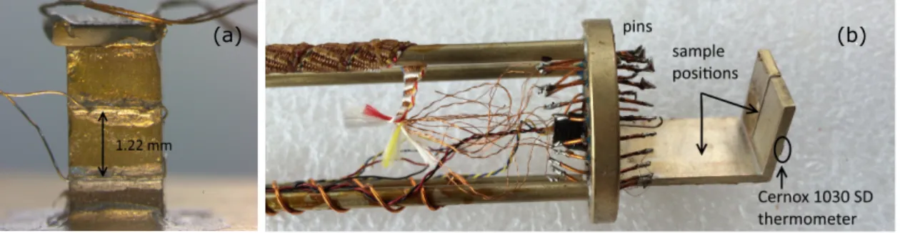
be measured, but an exact determination of temperature difference ∆T is quite challenging. Two different approaches are applied to measure ∆T . In the high- temperature regime for 5 K ≤ T ≤ 300 K, a thermocouple is used which consists of a chromel and a gold-iron alloy (0.07%Fe). Details about this technique can be found in Refs. 16, 32. However, the spin-ice physics only occurs in the low- temperature regime well below 5 K. Hence, the thermal conductivity measurements is obtained by another approach which is introduced in the following.

3.3.1 Low-temperature sample wiring

All measurements were performed on oriented single crystals and most suitable for

the steady-state method are bar-shaped samples with dimensions of ≈ 3 × 1.5 ×

1 mm ³ . Fig. 3.4 (a) shows a detailed view of an oriented single crystal Dy ₂ Ti ₂ O ₇

with dimensions 3 × 1.7 × 1.2 mm ³ that is completely wired for a steady-state

thermal-conductivity measurement at lowest temperatures. The typical ∆x varies

between 0.8 and 1.7 mm. The bottom of the sample is connected to a big copper

block that operates as the thermal bath. This block is fixed on the L-shaped

transport sample holder shown in Fig. 3.4 (b). Its L-shape allows to mount the

sample at different orientations with respect to the external applied magnetic field

direction. Fixing the sample on the bottom part leads to an applied magnetic field

along the longest dimension of the sample parallel to the heat current, i.e., ~j || H. ~

The lateral part of the holder is used to orient a magnetic field perpendicular to

the heat current, i.e., ~j ⊥ H, along another crystallographic direction. As can ~

be seen in Fig. 3.4 (a), platinum wires with a diameter of 0.05 mm, produced by

Heraeus [62], are attached to the sample at approximately one third and two thirds

Figure 3.5: Schematic drawing of the pseudo 4-wire technique used to wire the SMD heater in a thermal- conductivity measurement.

U I

pin plate

Heater SMD

copper wires manganin wires

of the longest dimension. Platinum is used due to its high thermal conductance (for measuring ∆T ) and its considerably high flexibility (even compared to copper wires). This flexibility eases to fix the wires to the backside of the small RuO ₂ thermometers (' 0.2 × 0.5 × 1 mm ³ ) with silver glue. These RuO ₂ thermometers are applied for the low-temperature thermal-conductivity measurements (0.25 K . T . 10 K) and exhibit a resistance of 5.3 kΩ at room temperature. Manganin wires electrically connect the RuO ₂ thermometers and the SMD heater to the pins of the sample holder, see Fig. 3.4 (a). Here, manganin is utilized due to its sufficient electrical conductivity but very low thermal conductivity. Thus, the majority of the heat provided by the SMD heater flows homogeneously through the sample into the bath instead of dissipating through the attached wires. This effect is even enhanced by spooling comparably long wires to connect the heater and the RuO ₂ thermometers. The accuracy of the thermometers is not affected by the growing electrical resistance because the 4-wire technique is applied.

Due to the rather high electric resistance of the manganin wires (' 60−100 Ω) which electrically connect the heater, it is not possible to prevent them from producing a certain amount of heating power in the experiment. In order to account for this additional amount of heating power, a pseudo 4-wire technique is applied to wire the heater. This wiring technique is depicted in Fig. 3.5. As can be seen, the heater is wired with 3 manganin cables to the pin sheet. Then, the pin of the single connection to the heater is connected to a fourth pin with a short copper wire.

This method is equivalent to the standard 4-wire resistivity measurement of the red dashed box. Consequently, the resistance of the heater and of one supply cable is measured. The idea is that half of the heat produced by the wires is transferred to the sample and the other half to the bath. Therefore, the total heating power can be calculated by the sum of the power of the heater and of one manganin cable.

The magnitude of the possible error σ can be estimated via σ ≤

heater

≈ _{1−70 kΩ} ^{100 Ω} .

3.3 Thermal conductivity

Adhesives

Due to different requirements for the thermal and electrical properties of the various parts which are assembled in wiring a sample for a heat-transport measurement in the low-temperature regime, it is essential to choose suitable adhesives. The choice depends on whether the sample is an insulator or metallic, on the samples’

compatibility with solvents and on the required mechanical stability. The industry offers a large number of products with different properties. This is a list of the adhesives that were used for wiring the crystals:

• Silver Glue:

Leitsilber G3303A Plano GmbH (silver glue) is a solvent-based glue con- taining silver particles [63]. It is both a good thermal and electrical conductor.

In wiring a sample, it is generally applied to mount the 0.05 mm platinum wires at two levels of the crystal, as can be seen in Fig. 3.4 (a). In this process, a da Vinci Maestro Tobolsky-Kolinsky 10/0 brush [64] is utilized to bring a narrow line of silver glue onto the wires which are stretched over the sample. The spin-ice crystals are insulating and, thus, silver glue could also be employed to fix the samples to the thermal bath. Furthermore, it was partly applied to mount the SMD heater on top of the crystals. The silver glue is highly soluble by solvents like acetone which is a clear advantage. In Ref. 16, an arising mechanical instability of the spin-ice crystals mounted with Leit- silber G3303A in an external magnetic field is reported originating from an arising torque for particular field directions. However, it turned out that the stability is sufficient.

• VGE 7031 Varnish:

VGE-7031 Insulating Varnish possesses electrical and bonding proper- ties which make it an applicable adhesive for heat-transport measurements.

At cryogenic temperatures, it is electrically insulating and exhibits a suffi- ciently large thermal conductivity of 0.062 W/mK at 4.2 K and 0.034 W/mK at 1 K [65]. The varnish can be air-dried within 1-2 hours and it can be additionally baked after assembling all parts in order to reach the maximum stability. It is completely solvable in aceton and ethanol. The VGE-7031 Insulating Varnish was partly used to mount the SMD heater on top of the samples. In the case of metallic samples, it is a convenient alternative to mount the crystals on the thermal bath.

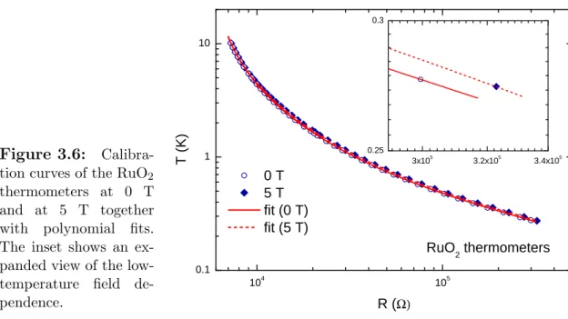
3.3.2 Calibration of RuO ₂ thermometers

The RuO ₂ thermometers are calibrated in advance of every single thermal-

conductivity measurement in the low-temperature regime. This is required because

Figure 3.6: Calibra- tion curves of the RuO ₂ thermometers at 0 T and at 5 T together with polynomial fits.

The inset shows an ex- panded view of the low- temperature field de- pendence.

1 0 ⁴ 1 0 ⁵

0 . 1

1

1 0

0 T 5 T f i t ( 0 T ) f i t ( 5 T )

T ( K )

R ( Ω)

R u O

2

t h e r m o m e t e r s

3 x 1 0⁵ 3 . 2 x 1 0 ⁵ 3 . 4 x 1 0 ⁵

0 . 2 5 0 . 3

their characteristics slightly change by every sample preparation and installation into the cryogenic environment. The calibration is performed in a separate run against the Cernox 1030 SD thermometer of the sample holder, see Fig. 3.4 (c). A characteristic calibration curve of the temperature T as a function of the resistance R of one RuO ₂ thermometer is shown in Fig. 3.6. It reveals a clear magnetic-field dependence for temperatures below ' 1 K, see inset. The measured curves are fitted by polynomials of degree 5–7 (solid and dashed red lines). A linear interpolation is used to calculate the field dependence between the measured fields which is found to be a good approximation [16, 32, 66]. In addition, the quality of the calibration can be improved by separately fitting the data in the low- temperature (0.25–2 K) and in the high-temperature regime (1.6 K–10 K). Then, the calibrations have to be switched in the overlapping temperature range.

3.3.3 Measurement instruments

Several instruments are available to measure the resistances R of the thermometers and to apply a power P to the sample heater. Here, a list of the instruments applied for the thermal-conductivity measurements is given:

• Resistance bridges

The Lakeshore 370 [65] is an AC resistance bridge which measures the resistance of the sample-holder thermometer and of the RuO ₂ thermometers.

The Lakeshore 370 is set to auto-range resistance and to voltage excitation

mode. It turned out that a voltage excitation of 632 µV is suitable in the

3.4 Thermal expansion and magnetostriction

capacitorplates

CuBe

springs sample

screw fixed

movable

Figure 3.7: Schematic drawing of a thermal expansion/magnetostriction cell with an assembled sample adapted from Ref. 68. The fixed and the movable part are connected via CuBe springs. The length change of the sample is calculated by the measured change in the capacitance.

temperature range from 0.25 K up to about 10 K. This excitation is low enough to prevent self-heating by the thermometers and it is high enough for low-noise data up to 10 K.

• Keithley instruments

A current source and a voltmeter are employed to measure the applied power to the SMD heater. It turned out that a Keithley 2182 nanovoltmeter [67]

and a Keithley 6220 current source [67] yield the best accuracy. However, the resolution of the Keithley 182 is still sufficient. The fast operation of a Keithley 6220 is a clear advantage compared to a Keithley 2400 .

3.4 Thermal expansion and magnetostriction

The length change ∆L

along the crystallographic axis i of a crystal can be mea-

sured as a function of the temperature (thermal expansion) or the magnetic field

(magnetostriction). The most common method to detect small length changes is

the capacitance dilatometry. Based on the original design in Ref. 69, different

setups have been developed [68, 70, 71]. A schematic drawing of a thermal ex-

pansion/magnetostriction cell is shown in Fig. 3.7. Its design is similar to the

low-temperature capacitance dilatometer which was applied to obtain the magne-

tostriction data in this thesis. In general, these setups consist of a fixed and a

movable part which are connected via springs. The crystal is clamped with a screw

between both parts and the length change ∆L can be calculated by the change in the capacitance ∆C via

∆L = ₀ πr ² 1

C − 1 C ₀

(3.3) with the starting capacity C ₀ , the vacuum permittivity ₀ and the radius r of the smaller capacitor plate which is shielded by the grounded movable part to prevent stray fields, see Fig. 3.7. In the experiment, ∆C is measured with a commercial AC capacitance bridge ( AH2550/2500 by Andeen Hagerling) that operates at a fixed frequency of 1 kHz. Length changes down to 10

m can be resolved because ∆C strongly increases for small distances between the plates and due to the high resolution of the capacitance bridges. The thermal expansion coefficient α or magnetostriction coefficient λ can be calculated numerically from the length change ∆L via

α = 1 L ₀

∂∆L(T, H)

∂T , λ = 1 L ₀

∂ ∆L(T, H )

∂H (3.4)

with the initial length L ₀ of the sample.

3.5 Specific heat

In Chap. 7.2, specific heat data of the dilute spin-ice materials (Dy _1−x Y

) ₂ Ti ₂ O ₇ are presented which were obtained using a custom home-built low-temperature calorimeter. This low-temperature calorimeter was built by O. Breunig during his diploma thesis [72]. The low-temperature physics of the (Dy _1−x Y

) ₂ Ti ₂ O ₇ crystals strongly vary with its dilution x and, thus, two different methods were acquired to obtain the specific heat data for all systems. The choice of the method depends on the equilibration properties. The relaxation method is a standard technique and it is applicable if the internal equilibration of the phononic and magnetic subsystems in a crystal are much faster than the equilibration to the bath. At very low temperatures T . 0.5 K, the specific heat of pure and weakly dilute spin ice (Dy _1−x Y

) ₂ Ti ₂ O ₇ with x . 0.1 has to be measured using another approach due to the long-time internal equilibration of the magnetic subsystems [11, 14, 20]. This approach is introduced in Sec. 3.5.2

3.5.1 Relaxation method

One of the standard methods to determine the specific heat of a crystal is the

relaxation-time method and a schematic drawing of the experimental setup is shown

in Fig. 3.8 (a). The sample is fixed on a sapphire platform by a small amount of

3.5 Specific heat

bath K

, t

K

, t

sample

thermometer heater

sapphire platform

C

K

, t

C

∼ ( e x p ( - ( t - t

) / τ

) )

t

∆ T ( t )

T

∼ ( 1 - e x p ( - ( t - t

1

) / τ

) )

∆ T

m a x

+ T

0

T e m p e ra tu re

t i m e t

(a) (b)

Figure 3.8: Panel (a): schematic drawing of the specific heat setup adapted from Ref. 14. Panel (b): raw data of the relaxation method. At time t ₁ , the heater is switched on and T (t) = ∆T (t) + T ₀ increases. At t ₂ , the heater is switched off and T(t) relaxes back towards T 0 with a time constant τ = C/K 1 .

grease ( Apiezon N ) which solidifies upon cooling below room temperature. Sap- phire is a suitable material due to its small heat capacity but large thermal con- ductivity at low temperatures. K ₂ denotes the coupling between the platform and the sample via the grease. A thermometer ( Cernox 1030 BC ) and a SMD heater (R ' 27.3 kΩ at room temperature) are mounted to the platform by VGE-7031 Insulating Varnish [65]. The whole setup has a defined coupling to the bath via a thin platinum wire with the thermal conductance K ₁ . Another established method to measure the specific heat is the quasi-adiabatic heat pulse method which, however, was not applied in this thesis. Details can be found in Refs. 72, 73. In contrast to the relaxation method, it requires K ₁ to be as small as possible ¹ . For the relaxation method, it is assumed that K ₂ = ∞. The schematic tempera- ture dependence of a single heat pulse as function of time is shown in Fig. 3.8 (b).

Within the Heliox VL temperature controller, T ₀ does not equal the bath tem- perature. Instead, T ₀ is stabilized by an offset power P ₀ of the heater which yields a faster temperature control of the sample temperature and lowers the impact of fluc- tuations of the Heliox VL . When the stabilization criteria at T ₀ are fulfilled, the heating power is increased at t ₁ by applying an additional power ∆P to the heater.

Hence, T (t) = ∆T (t) + T 0 rises. At time t 2 , the additional power ∆P is removed and T (t) relaxes back towards T ₀ . With K ₂ = ∞ and T = T _sample = T _platform , it

1

Note that a finite K

is required to provide a finite cooling power.

follows from the first law of thermodynamics, that

∆Q = C dT. (3.5)

From Eq. (3.5), a differential equation can be extracted and it is given by

C dT = ∆P dt − K ₁ (T − T ₀ )dt. (3.6) Eq. (3.6) is solved by ∆T (t) _heat and ∆T (t) _cool for the heating and relaxation curves, namely [73]

∆T (t) _heat = ∆P/K ₁ (1 − exp(−(t − t ₁ )/τ ₁ )) (3.7)

∆T (t) _cool = ∆P/K ₁ exp(−(t − t ₂ )/τ ₁ ). (3.8) In the limit of t → ∞, the steady-state equation yields ∆P/K ₁ = ∆T (t → ∞) =

∆T _max . The relaxation time τ ₁ is related with the heat capacity via τ ₁ = C/K ₁ . The raw data of the heating and relaxation curves are fitted separately which yields K ₁ and τ ₁ . Note that reliable results are only obtained if τ ₁ determined from the heating and from the relaxation curve are identical. The heat capacity of the addenda is measured in a separate run and is subtracted from the data in the same way as the heat capacity of the Apiezon N grease which is known from literature [74, 75]. In the data analysis, so-called τ ₂ effects can also be taken into account which arise from an imperfect coupling of the sample to the platform via K ₂ [73]. In general, τ ₂ is defined by the coupling of the sample to the platform via the low-temperature Apiezon N grease. In order to minimize these effects in the experiment, it has to be ensured that the sample is properly attached with the grease and with a large cross section on the platform.

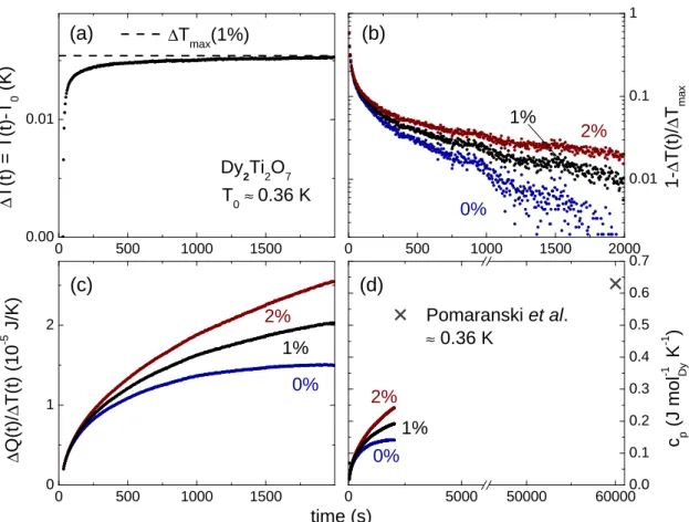
3.5.2 Heat-flow method

For T . 0.5 K, long-term internal equilibration has been observed in Dy ₂ Ti ₂ O ₇ [11, 14, 20]. This is related to the fact that the relaxation times τ

between the different sub-systems C _P (phononic) and C _M (magnetic) and, especially within C _M become very large compared to the equilibration with the platform τ ₂ and with the bath τ ₁ , see Fig. 3.8 (a). In order to account for these long-term equilibration pro- cesses, a new approach has been developed which was named ”constant heat-flow method” [14]. It analyzes the heating curves over long timescales and is equiva- lent to the method applied by Pomaranski et al. [20, 76] in which the specific heat is derived from the long-time temperature relaxation curves. The constant heat- flow method only differs from the relaxation method by the fact that the raw data

∆T (t) = T (t) − T ₀ are recorded for a longer period of time and an exponential

3.5 Specific heat

0 5 0 0 1 0 0 0 1 5 0 0

0 1 2

1 % 2 %

0 % ( c )

∆ Q (t )/ ∆ T (t ) (1 0

J /K )

t i m e ( s )

0 5 0 0 1 0 0 0 1 5 0 0 2 0 0 0

0 . 0 1 0 . 1

1

( b )

1 % 2 %

1 - ∆ T (t )/ ∆ T

0 %

0 5 0 0 1 0 0 0 1 5 0 0

0 . 0 0 0 . 0 1

D y

T i

2

O

T

≈ 0 . 3 6 K

∆ T

m a x

( 1 % )

∆ T (t ) = T (t )- T

( K )

( a )

0 5 0 0 0 5 0 0 0 0 6 0 0 0 0 0 . 0

0 . 1 0 . 2 0 . 3 0 . 4 0 . 5 0 . 6 0 . 7

P o m a r a n s k i e t a l . _≈ 0 . 3 6 K

( d )

1 % 2 %

0 %

c ( J m o l K )

Figure 3.9: Panel (a): heating curve ∆T (t) = T (t) − T 0 of Dy 2 Ti 2 O 7 at T ≈ 0.36 K. The dashed black line represents ∆T _max (1%), see text. Panel (b):

1 − ∆T(t)/∆T _max for different ∆T _max . Panel (c): constant heat-flow method for different ∆T max . Panel (d): comparison of c

for different ∆T max and with results from Pomaranski et al. [20].

increase of ∆T (t) is not required. In analogy to the relaxation method, the sample and the platform are raised to a constant temperature T ₀ above the thermal reser- voir by an offset power. Then, an additional power ∆P is applied to the heater.

Exemplary raw data ∆T (t) = T (t) − T ₀ of Dy ₂ Ti ₂ O ₇ at T ≈ 0.36 K are shown in Fig. 3.9 (a). In order to ensure measurable variations in ∆T (t) over long times, the thermal coupling K ₁ to the bath has to be weak. As can be seen, this setup allows for measurements up to about 2000 s whereas the variations in ∆T become too small for t > 2000 s. In order to obtain the heat capacity from the raw data,

∆T _max = ∆T (t → ∞) has to be determined which is obtained by an exponential

fit to the heating curve in the limit t → ∞ in the relaxation method. Within the

constant heat-flow method, ∆T _max can either be fixed by ∆T (2000 s) or by an esti-

mation of ∆T (t → ∞). Fig. 3.9 (b) presents the time-dependence of ∆T (t) in the

representation 1 − ∆T (t)/∆T _max whereas ∆T _max is increased by 0%, 1% and 2%

with respect to ∆T (2000 s). With increasing ∆T _max , 1 − ∆T (t)/∆T _max is enhanced and exhibits a linear decrease in the long-time limit. An exemplary ∆T _max , which is raised by 1% with respect to ∆T (2000 s), is depicted as the black dashed line in panel (a). As can also be seen in panel (b), 1 − ∆T (t)/∆T _max of Dy ₂ Ti ₂ O ₇ shows a clearly non-linear decrease in the semi-logarithmic representation which makes the standard relaxation method inapplicable. In order to calculate the specific heat via the constant heat-flow method, the heat applied to the sample as a function of time is obtained from the difference

∆Q(t) = ∆P t − Z

K 1 ∆T (t)dt (3.9)

between the total amount of heat ∆P t provided by the heater and the heat flown from the platform to the bath via R

K ₁ ∆T (t)dt with K ₁ = ∆P/∆T _max . Thus, the thermal coupling to the bath K ₁ = ∆P/∆T _max is related to the estimation of

∆T max . The heat capacity follows via

C(t) = ∆Q(t)/∆T (t) (3.10) which is shown in Fig. 3.9 (c) for different ∆T _max . Naturally, ∆Q(t)/∆T (t) cal- culated with ∆T _max (0%) saturates for t → 2000 s. It turns out that C(t) =

∆Q(t)/∆T (t) is highly sensitive to the estimation of ∆T _max . Thus, a reason- able estimation of ∆T _max is required. In the analysis of the raw data of this thesis, ∆T _max = ∆T (t → ∞) was obtained by slightly raising ∆T (2000 s) by 0.5-1% such that 1 − ∆T (t)/∆T _max reveals a linear decrease in the long-time limit but almost vanishes, see panel (b). The constant-heat flow method was applied for (Dy _1−x Y

) ₂ Ti ₂ O ₇ with x = 0–0.1 in the low-temperature regime T . 0.5 K.

Fig. 3.9 (d) compares the results of the specific heat c

for different ∆T _max ob- tained via the constant heat-flow method to c

determined by Pomaranski et al. [20]. This group applies an equivalent method which analyzes the temper- ature relaxation curves over 6 · 10 ⁴ s after the sample temperature is raised by

≈ 5–10% above the base temperature T ₀ . A weak link of Pt ₉₁ W ₉ with conductance K/T ≈ 2.8 · 10

W/K ² was used to connect the sample to a thermal reservoir in order to ensure measurable variations in ∆T (t) over these long timescales. This ap- proach reduces uncertainties of ∆T _max but it is extremely sensitive to the stability of the base temperature T ₀ which has to be stabilized over the whole time period of a single ∆T (t) curve (6 · 10 ⁴ s). At 0.36 K, c

of Pomaranski et al. exceeds the result obtained via the constant heat-flow method with ∆T _max (1%) by a factor of 3.

This deviation might stem from a too large coupling to the thermal reservoir which

restricted the measurements of ∆T (t) to 2000 s in the experiment. However, it is

systematically shown that the determination of c

by integrating over these long

timescales bares several problems and already small uncertainties in T ₀ or ∆T _max

lead to large deviations of c

in the long-time limit.

3.6 Magnetocaloric effect

1 3 1 4

( P + P ) / 2 = K ⋅ ∆ T ( b )

P ( µ W )

T = 2 K

H | | [ 0 0 1 ]

- 2 - 1

0 1 2 D y

T i

O

u p

d o w n ( a )

0 . 4 K 0 . 5 K 1 K 2 K

(T -T

)/ T

( % )

0 . 0 0 . 5 1 . 0 1 . 5

0 . 1 0 . 2

H | | [ 1 1 1 ] ( c )

µ

H ( T ) ( P + P ) / 2

K ⋅ ∆ T ( e m p t y s a m p l e h o l d e r )

T = 0 . 4 K

Figure 3.10: Panel (a): relative deviation from the target temperature (T − T ₀ )/T ₀ of Dy ₂ Ti ₂ O ₇ at various temperatures. Panel (b): antisymmetric curves of P with increasing and decreasing field at 2 K. The red line represents the symmetric contribution K∆T calculated from (P

+ P

)/2. Panel (c): non- antisymmetric curves of P at 0.4 K. The background contribution K∆P (green line) was determined in a separate run.

3.6 Magnetocaloric effect

This section introduces the magnetocaloric effect which was measured for pure and dilute spin ice (Dy _1−x Y

) ₂ Ti ₂ O ₇ with x = 0 and 0.75 at different temperatures. A special analysis of the magnetocaloric effect data allows to determine the change of entropy as a function of the external magnetic field. More information about this field-dependent effect and materials exhibiting magnetocaloric properties can be found in an review article [77]. The experimental data of the magnetocaloric effect were obtained using the low-temperature calorimeter which is also applied for the specific heat measurements, see a schematic drawing in Fig. 3.8 (a). The sam- ple is equally mounted on the sapphire platform by Apiezon N low-temperature grease. Then, the sample temperature T is raised to a target value T ₀ above the thermal reservoir of the Heliox VL by an SMD heater in zero magnetic field.

When T is stabilized at T ₀ , the magnetic field is continuously increased and then

decreased meanwhile a PID routine steadily controls and stabilizes T to the target

temperature. Typical curves of the relative temperature stability (T − T ₀ )/T ₀ as a function of the field for Dy ₂ Ti ₂ O ₇ at different target temperatures T ₀ are depicted in Fig. 3.10 (a). It turns out that the deviation from the target temperature amounts to about 1.2% in maximum for this material. This is a result of the comparably large heating/cooling of the sample due to the large magnetocaloric effect of the Dy ³⁺ ions with µ = 10µ B . These deviations are clearly smaller for the dilute system x = 0.75 due to the replacement of magnetic ions by non-magnetic yttrium.

The derivation of the change of entropy ∆S(H) follows Ref. 73. In general, the entropy S = S(H, T ) of a system depends on the temperature and the magnetic field. As a consequence, the differential is given by [78]

dS = ∂S

∂T

dT + ∂S

∂H

dH. (3.11)

As T is kept constant, the first term in Eq. (3.11) vanishes and the internal en- ergy U (S, V, N ) of a magnetic system at constant volume and particle number is determined by

dU = T · dS = T ∂S

∂H

dH. (3.12)

The power P of the heater is adjusted to keep T constant. Furthermore, the heat provided by the heater and the heat flown to the bath via the conductance K equal the differential of the internal energy via

dU = P (H)dt − K(H)∆T dt. (3.13)

Eq. (3.12) and (3.13) can be combined to determine the change of the entropy as a function of the magnetic field

P (H) − K(H)∆T

γ = T ∂S

∂H

(3.14) with the sweep rate of the magnetic field γ = dH/dt. The heating power P (H) can be separated into a background contribution and a contribution of the change of entropy whose sign depends on the field sweep direction. In the following, P

denotes the heating power with increasing magnetic field and P

with decreasing field. Thus, Eq. (3.14) can be rewritten to

P

(H) = K(H)∆T ± |γ|T ∂S

∂H

. (3.15)

The first term in Eq. (3.15) represents the background contribution K (H)∆T and

accounts for the heating power to reach the temperature difference ∆T between

the sample and the thermal reservoir. K(H)∆T is independent of the field-sweep