Thermodynamics and transport properties of the ferromagnetic metal SrRuO 3 and
the frustrated magnet Cs 3 Fe 2 Br 9
I n a u g u r a l - D i s s e r t a t i o n
zur
Erlangung des Doktorgrades
der Mathematisch-Naturwissenschaftlichen Fakultät der Universität zu Köln
vorgelegt von Daniel Brüning aus Menden (Sauerland)
Köln, 2020
Prof. Dr. Markus Braden Vorsitzender der Prüfungskommission: Prof. Dr. Simon Trebst
Tag der mündlichen Prüfung: 26.06.2020
Contents
1 Introduction 1
2 Theory 5
2.1 Electric transport . . . . 5
2.1.1 Longitudinal transport . . . . 6
2.1.2 Transverse transport . . . . 8
2.2 Magnetism . . . . 14
2.2.1 Magnetic exchange . . . . 15
2.2.2 Magnetic order . . . . 17
2.2.3 2D triangular lattice . . . . 21
2.2.4 Hexagonal closed packed structure . . . . 22
3 Experimental 25 3.1 Cryogenic setups . . . . 26
3.2 Magnetic field . . . . 27
3.3 Magnetization . . . . 28
3.3.1 SQUID magnetometer . . . . 28
3.3.2 Pick-up techniques . . . . 29
3.3.3 Faraday magnetometer . . . . 30
3.4 Thermal expansion and magnetostriction . . . . 36
3.5 Specific heat and magnetocaloric e ff ect . . . . 39
3.6 Pyrocurrent . . . . 44
3.7 Electric transport properties . . . . 45
4 SrRuO 3 49 4.1 Introduction . . . . 50
4.2 SrRuO 3 literature . . . . 52
4.3 Criticality of the ferromagnetic phase transition . . . . 56
4.4 Magnetic anisotropy . . . . 62
4.5 Magnetoelastic coupling and shape-memory e ff ect . . . . 67
4.6 Electric transport properties . . . . 72
4.7 Magnetic excitations . . . . 80
4.8 Conclusion . . . . 82
5 Cs 3 Fe 2 Br 9 85 5.1 Introduction . . . . 86
5.2 Crystal growth and structure . . . . 86
5.3 Literature about related materials . . . . 88
5.4 Zero-field characterization of Cs 3 Fe 2 Br 9 . . . . 94
5.4.1 Thermodynamic properties . . . . 94
5.4.2 Neutron scattering . . . 101
5.4.3 Magnetic structure . . . 102
5.5 Magnetic-field response . . . 107
5.5.1 Magnetic field ⊥ c . . . 107
5.5.2 Magnetic field k c . . . 110
5.6 Dielectric constant and electric polarization . . . 120
5.7 Comparison to related models and materials . . . 123
5.8 Conclusion . . . 127
6 Summary 129 A Appendix 133 A.1 Berry phase . . . 133
A.2 Full data sets Cs 3 Fe 2 Br 9 . . . 136
A.3 Dy 2-x Ho x Ti 2 O 7 . . . 141
A.4 LiFe(WO 4 ) 2 . . . 146
A.5 Ba 1-x Sr x Co 2 V 2 O 8 . . . 148
A.6 Küchler dilatometer cell e ff ect . . . 152
A.7 Magnetometer cell e ff ect in the gradient cryostat . . . 153
List of Figures 155
List of Tables 159
Bibliography 161
Danksagung 175
Contents
Abstract 177
Kurzzusammenfassung 179
Publikationen 181
Erklärung 183
1 Introduction
Magnetism fascinated humans ever since its discovery. From the first technical application as a compass [1] through the use for data storage in information technology [2] to possible future applications like spintronics [3], magnetism plays an important role in our everyday life and is a dominant engine of the technological progress. The spirit of understanding the underlying mechanisms fascinated and is still fascinating uncountable scientists.
Magnetic materials mostly consist of elements with partially filled shells. Very di ff erent magnetically ordered states exist, ranging from ferromagnetic metals like iron, cobalt, and nickel to antiferromagnetic oxides like MnO, FeO, CoO, and NiO [4], to complex magnetic systems like skyrmions in MnSi [5], to name a few examples. Fundamental interactions that play the most important role in such magnetic materials are coulomb interaction, ex- change interaction, and spin-orbit coupling. In materials with 3d transition-metal ions, the magnetism is typically dominated by electron-electron correlations. The increased or- bital size of 4d and 5d ions reduces the energy scale for the electron correlations, while the spin-orbit interaction grows to a comparable level. The interplay of these interactions yields many interesting phenomena. An example for systems where the spin-orbit inte- raction is very important are Kitaev materials [6] with a spin-liquid ground state which may be realized in α-RuCl 3 [7] and Na 2 IrO 3 [8, 9]. Another candidate was Ba 3 CeIr 2 O 9 [10], which turned out to be a so-called cluster material with Ir 2 O 9 bi-octahedra and strong spin-orbit coupling [11]. This thesis studies two related materials in this context, the first is the ferromagnetic metal SrRuO 3 with sizable spin-orbit interaction. The second is the new material Cs 3 Fe 2 Br 9 , which is an analogon to the cluster material Ba 3 CeIr 2 O 9 but with weak spin-orbit interaction in the Fe 2 Br 9 bi-octahedra.
Ruthenates became scientifically popular by the observation of superconductivity in
Sr 2 RuO 4 [12]. The material itself is not interesting from a technological perspective be-
cause of its low transition temperature, but due to its structural similarity to the high-T C
cuprates like YBa 2 Cu 3 O 7−δ [13]. Both materials consist of layers of corner-sharing MO 6
octahedra with M = Ru, Cu, respectively. The pairing symmetry in Sr 2 RuO 4 has been dis-
cussed controversially since the discovery of superconductivity in this material. There is
evidence for spin-triplet Cooper pairs [14] but only recently new insights raised questions
about this result [15]. Ferromagnetic fluctuations have been proposed as the pairing me- chanism. This motivated studies of the closely related ferromagnetic metal SrRuO 3 , which is the infinite-layered member (n = ∞) of the Ruddlesden-Popper series Sr n−1 Ru n O 3n + 1 , where the octahedra are also corner-sharing in the third dimension. SrRuO 3 is widely stu- died in thin films and also used as a ferromagnetic layer in perovskite heterostructures [16].
Another hot topic in solid-state physics is topology. Recently, the extraordinary behavior of the anomalous Hall conductivity and of the temperature dependence of magnetic exci- tations have been explained with the topology of the band structure [17, 18]. The presence of sizable spin-orbit coupling and Weyl points close to the Fermi energy yield an addi- tional contribution to the electron velocity based on the concept of the Berry curvature.
In Cologne, a recipe was found to synthesize large high-quality single crystals with the floating-zone technique [19]. This work provides a detailed study of these single crystals.
The thermodynamic characterization yields new insights in the criticality of the ferromag- netic phase transition. The magnetic anisotropy is clarified and a previously unknown shape-memory e ff ect of SrRuO 3 is found. The combined analysis of electric transport and magnetization measurements gives new insights in the anomalous Hall e ff ect induced by the Berry-curvature e ff ect. Its signature is found in neutron-scattering experiments. The reported analysis is improved by showing the anomalous temperature dependence not only for the magnon gap but also for the sti ff ness.
The second material studied in this work is the new potential cluster material Cs 3 Fe 2 Br 9 . Magnetic cluster materials contain separated structural building blocks of highly-connected metal coordination polyhedra. Inside these units, the metal-metal interaction is dominant and the metal-metal distance can be shorter than in the corresponding elemental metal [20]. The relative size of the intra-cluster and inter-cluster exchange determines the mag- netism of such materials. In Cs 3 Fe 2 Br 9 , the main building blocks are face-sharing Fe 2 Br 9
bi-octahedra arranged in triangular layers that are stacked to build a hexagonal structure.
Ba 3 CeIr 2 O 9 is structurally very similar and consists of face-sharing Ir 2 O 9 bi-octahedra.
In this material, the iridium ions form molecular orbitals inside each bi-octahedron with
strong spin-orbit coupling [11]. Cs 3 Cr 2 Br 9 and Cs 3 Cr 2 Cl 9 also consist of face-sharing
Cr 2 X 9 bi-octahedra [21] and are isostructural to Cs 3 Fe 2 Br 9 . However, in these 3d spin
systems the spin-orbit interaction is only a small perturbation. The chromium ions are
strongly bound so that their antiferromagnetic exchange dominates, leading to a singlet
ground state. An applied magnetic field reduces the energy of the magnetic states and
induces a phase transition to a magnetically ordered state [22]. Interestingly, Cs 3 Fe 2 Br 9
shows antiferromagnetic magnetic order. The phase diagram is studied with thermal ex-
pansion, magnetostriction, and magnetization. These studies also make use of high-field
facilities with the capability of magnetic fields up to 57 T. The magnetic ground-state struc- ture is determined by neutron scattering. The results are compared to related materials and numerical predictions for appropriate model Hamiltonians. This allows first approximati- ons of the underlying coupling strengths.
The thesis is structured as follows. Chapter 2 introduces required theoretical concepts,
with special focus on transverse transport mechanisms and numerical predictions for mag-
netic model Hamiltonians. The following introductory Chapter 3 presents the experimental
techniques and setups used in this work. Chapter 4 presents a study of the magnetoelas-
tic coupling, criticality, and electric transport of floating-zone-grown single crystals of the
ferromagnetic metal SrRuO 3 . The new potential cluster material Cs 3 Fe 2 Br 9 is studied in
Chapter 5 via multiple thermodynamic quantities. The obtained magnetic structure and
the magnetic phase diagram are compared to related materials and model systems.
2 Theory
Contents
2.1 Electric transport . . . . 5
2.1.1 Longitudinal transport . . . . 6
2.1.2 Transverse transport . . . . 8
2.2 Magnetism . . . . 14
2.2.1 Magnetic exchange . . . . 15
2.2.2 Magnetic order . . . . 17
2.2.3 2D triangular lattice . . . . 21
2.2.4 Hexagonal closed packed structure . . . . 22 This chapter introduces some basic models and concepts that are employed in the dis- cussion and interpretation of experimental results on SrRuO 3 and Cs 3 Fe 2 Br 9 in Chapters 4 and 5. Starting from a basic motivation of electric transport and the underlying scattering e ff ects, special attention is paid to transverse transport mechanisms. Besides the extrinsic e ff ects skew scattering and side jump, especially the intrinsic e ff ect caused by spin-orbit coupling and the topology of the band structure is discussed. Furthermore, magnetic ex- change mechanisms and magnetic order are introduced. Finally, analytical and numerical predictions for the magnetic order on the 2D triangular lattice and the hexagonal closed packed structure are presented.
2.1 Electric transport
The theory of electric transport can often be captured e ffi ciently by a straight-forward,
semiclassical picture. While the topic is extensively covered in many text books [23],
here, the central results to establish the sign convention used throughout the thesis are
recapitulated briefly.
An electric current density j through a material induces a voltage drop per length U.
The quantities are connected via the resistivity tensor ρ through
U x
U y
=
ρ xx ρ xy
ρ yx ρ yy
·
j x
j y
(2.1)
or equally formulated in terms of the electric field E and the conductivity σ with
j x
j y
=
σ xx σ xy
σ yx σ yy
·
E x
E y
. (2.2)
Combining Eqns. (2.1) and (2.2) obtains
σ xx σ xy
σ yx σ yy
·
ρ xx ρ xy
ρ yx ρ yy
=
1 0 0 1
,
and especially σ xy = ρ
2−ρ
xy xx+ ρ
2xy.
In the following, a current along the x-axis is considered which is the typical case in a transport measurement and thus j y = 0. Equation (2.1) then simplifies to Ohm’s law for the longitudinal transport and the transverse Hall transport yields
U y = ρ yx · j x .
2.1.1 Longitudinal transport
The longitudinal transport is described by the conductivity σ xx . According to the Drude- Sommerfeld transport theory, quasi-free electrons are scattered inside the material which limits the transport. This yields a conductivity of
σ xx = n e e 2 τ m e
,
with the density of electrons n e , their charge e, mass m e , and the time constant between two scattering events τ. For a metal, all entities, except τ, can be considered temperature independent. Thus, the conductivity only depends on the temperature dependence of the scattering e ff ects. With the Fermi velocity v F , a mean free path l between two scattering events can be defined as
l = v F · τ .
2.1 Electric transport
Let us assume a free-electron gas with a spherical Fermi surface and the Fermi velocity v F = m ~
e·
3π 2 n e
1/3
. For the resistivity follows
ρ(T ) = ~
3π 2 1/3
e 2 · 1 ln 2/3 e
.
According to Io ff e, Regel [24], and Mott [25] there is a high-temperature saturation limit for the resistivity ρ sat in usual metals, if the scattering length is comparable to the lattice constant l ∼ a:
ρ sat = 1.29 · 10 18
n 2/3 a µ Ω cm .
At lower temperatures, di ff erent scattering mechanisms are relevant, which show di ff erent temperature dependencies:
• Scattering on defects: A constant defect density implies a constant scattering time.
This yields the so-called residual resistivity ρ 0 = ρ(T = 0 K), which is often used to quantify the quality of a sample.
• Electron-phonon-scattering: Phonons that describe excitations of the lattice, de- stroy the periodicity of the lattice, and, thus, they lead to scattering with conduction electrons. Their contribution can be described by the Bloch-Grüneisen formula [26]
ρ el-ph (T ) ∝ T 5 θ D 6
θD
Z
T0
x 5
(e x − 1) (1 − e −x ) dx ,
with the Debye temperature θ D . Because the phonon density increases with tempe- rature, so does the scattering. For high and low temperatures relative to the Debye temperature this yields the limits
ρ el-ph (T ) ∝
T 5 for T θ D
T for T θ D .
• Electron-electron scattering: The electron-electron scattering is typically negligi-
bly in normal metals due to Pauli principle.
2.1.2 Transverse transport
The transverse transport consists of the normal or ordinary Hall e ff ect (NHE) caused by a deflection of charge carriers due to a magnetic field [27] and also of an anomalous Hall e ff ect (AHE), which was found in ferromagnetic metals and that scales with the magneti- zation M [28]. The total Hall resistance
ρ xy (T, B) = ρ NHE xy + ρ AHE xy (2.3)
= R H (T )B ext + R AHE (T )µ 0 M(T, B ext )
contains the normal and anomalous Hall coe ffi cient R H and R AHE . The normal Hall coe ffi - cient of a single conduction band only depends on the charge carrier density n via
R H = 1
nq . (2.4)
Thus, the sign directly tells, whether the transport is dominated by electrons (negative charge q < 0 ⇒ R H < 0) or holes (q, R H > 0). Multiple bands with electron and hole carriers can compensate each other.
The anomalous Hall contribution contains intrinsic and extrinsic e ff ects. Intrinsic con- tributions are independent of impurities and consequently dissipationless [29], while ex- trinsic contributions base on spin-dependent scattering processes and thus depend on the impurity concentration. In the following, the possible e ff ects are discussed adapting the explanation from Ref. [23]:
Extrinsic processes
• Skew scattering:
In the following, electron scattering at an electric impurity potential φ imp in the back- ground of an external electric field E ext = −∇φ ext is considered. The spin of an elec- tron s = ~ 2 σ, where σ x =
0 1 1 0
, σ y =
0 − i
i 0
, σ z =
1 0
0 −1
are the Pauli matrices, interacts with both electric fields according to the spin-orbit exchange energy
E so = X
i
α (k × σ) · ∇φ i ,
where α = q ~ /2m 2 e c 2 . Furthermore, the total Hamiltonian of an electron contains the
2.1 Electric transport
potential energies E pot = P
i
qφ i and the kinetic energy:
H = ~ 2 k 2
2m + qφ ext + α (k × σ) · ∇φ ext + qφ imp + α (k × σ) · ∇φ imp . (2.5) Only the last two terms contain the potential of the impurity and can lead to skew scattering. Both contributions can scatter an electron from a state with momentum
k and spin quantum number s to another state k 0 , s 0 with the matrix element D k 0 , s 0
qφ imp + α (k × σ) · ∇φ imp k, s E
= V kk
0{δ s,s
0− iα k × k 0
· hs 0 |σ| si} . The first term results from spin-conserving scattering at the impurity, while the se- cond term occurs due to spin-orbit coupling. The sign of this term depends on the relative orientation of k × k 0 and the spin s. Figure 2.1 indicates the scenarios for elastic scattering of spins with two di ff erent spin orientations and incident moment k by an angle ± θ into k 0 or k 00 , respectively. In panel (a), k × k 0 is antiparallel to s, and, thus, it results in a larger matrix element than the scattering to k 00 . In panel (b), the spin is inverted and consequently k 00 becomes favorable. Because of this asym- metric scattering, a Hall voltage can occur. The scattering at these defects does not only influence the Hall signal but similarly contributes to the longitudinal resistance ρ xx . Obviously, in a spin-degenerate material both skew scattering contributions would compensate each other, and, thus, a preferred spin orientation is required.
Consequently, the Hall resistance has to be proportional to the spin-polarization of the charge carriers, as it is the case for a band ferromagnet (∝ M). Thus, the Hall resistivity induced by skew scattering follows
ρ AHE ∝ ρ xx M(B ext ) .
• Side Jump:
Another asymmetric scattering mechanism is called side-jump mechanism [30, 31].
Because elastic scattering is assumed (|k| = |k 0 |), the kinetic energy term of Eqn. (2.5)
is constant. Nonetheless, the spin-orbit exchange energy of the electron in the sta-
tic electric field changes according to E SO = α (k × σ) · ∇φ ext . In order to maintain
energy conservation, the potential energy E pot = qφ ext has to change accordingly. For
a linear external potential, i.e., φ ext = E · r, this results in a change of the scattering
parameter r. Thus, the side-jump e ff ect causes a vertical deflection δ, see Fig. 2.1(c),
which is typically of the order of 10 −14 to 10 −10 m [31]. The number of scattering
(a) (b) (c)
k k' k k''
s
k k''
k'
θ θ
k k' k k''
s k
k'' k'
E s
s
δ θ θ
Figure 2.1 Spin-dependent transverse scattering mechanisms. (a) and (b) illustrate the skew-scattering mechanism. For panel (a), electrons with moment k and spin s (s ⊥ k) favor elastic scattering to k 0 (up by angle θ) instead of k 00 (−θ), because k × k 0 is anti- parallel to the spin s. In panel (b), the spin is inverted and, thus, k 00 becomes favorable.
The effect requires a net spin polarization in order to be finite. The side-jump mechanism shown in (c) yields a deflection δ that depends on the spin direction resulting from energy conservation during a scattering process at an impurity in an external electric field E.
Figure adapted from Ref. [23].
events and also the size of the deflection are proportional to the longitudinal resisti- vity ρ xx . Furthermore, the e ff ect depends on the spin-polarization and, therefore, on the magnetization M. Thus, the side-jump mechanism yields
ρ AHE ∝ ρ 2 xx M(B ext ) . Intrinsic effects
An explanation for the anomalous Hall e ff ect was already proposed by Karplus and Lut- tinger in 1954 who suggested a contribution due to spin-split bands caused by spin-orbit coupling [32, 33]. This e ff ect should not depend on the impurity concentration (intrinsic).
The elementary explanation of their proposition is based on the concept of the Berry phase, which is explained in Appendix A.1. The explanation below follows Ref. [23].
For further reading see e.g. Refs. [34, 35]. We consider a system with parameter R that moves adiabatically in the phase space along a path Γ and starts in an eigenstate
| Ψ (t 0 )i = |m[R(t 0 )]i with the eigenenergy m (t 0 ) where m denotes the band index. The sy- stem remains in the time-dependent eigenstate |m(t)i. The phase di ff erence along the path consists of a dynamical and a geometrical part, see Appendix A.1. This phase
γ m ( Γ ) = Z
Γ
A m (R) · dR (2.6)
contains the Berry potential
A m (R) = i
*
m[R(t)]
d dt
m[R(t)]
+
.
2.1 Electric transport
This connects to the Berry flux or Berry curvature Ω m via
Ω m (R) = ∇ R × A m (R) . (2.7)
The path integral from Eqn. (2.6) can be rewritten to a surface integral using Stokes theo- rem and the Berry curvature
Z
S
Ω m (R) · nd ˆ 2 R .
Thus, the Berry phase can be understood as an Aharonov-Bohm phase induced by an e ff ective magnetic-flux density Ω m (R) in the parameter space. Still, the question about the origin of this flux density remains. Here, we focus on the spin-orbit coupling.
We assume Bloch waves Ψ m,k = e ik·r u m,k (r) with a lattice-periodic function u m,k (r). In k space, the position operator is R = i∇ k and the Hamiltonian
H (k) = H 0 (k) + V (R)
has eigenstates |u m (k)i with the eigenenergy m (k). The gradient of the potential V(R) results in a force
~ d k
dt = −i[k, H] = − ∂V
∂R .
This force is assumed to be small in order to result in an adiabatic motion, and, thus, in a drift of k along some path Γ . Appendix A.1 shows that this results in the Berry phase
γ m ( Γ ) = Z
Γ
A m (k) · dk .
The corresponding Berry curvature, see Eqn. (2.7), can now change the behavior of the charge carriers due to the potential. This can be shown by using the gauge transformation that compensates the Berry phase
X m = i∇ k + A m ( k) , H ˜ = H 0 + V (i∇ k + A m )
This transformation does not influence the force ~ k, but adds an additional term to the ˙
group velocity, which results from the Berry phase 1 :
~ v m = −i[X m , H] ˜ = ∇ k m (k) + ∂V
∂X m
!
× Ω m (k)
~ dk
dt = − i[k, H ˜ ] = − ∂V
∂X m
.
The additional term is called anomalous Luttinger velocity [32].
In an electric transport measurement, we apply an electric field E and additionally a magnetic field B. This results in the potential V = qE · X m and the modified equation of motion:
~ v m = ∇ k m (k) − qE × Ω m ( k)
| {z }
~v
AHE(2.8)
~ d k
dt = q [E + v m ( k) × B] . (2.9)
With the Boltzmann transport equation we can find the current density for B = 0 J q = 1
4π 3 Z
qv(k)
f 0 (k) + g( k)
d 3 k . (2.10)
Here, f 0 ( k) denotes the equilibrium Fermi distribution and g(k) = −qτv(k) · E(∂ f 0 /∂) the correction due to the electric field with the relaxation time τ. Without the anomalous Luttinger velocity, the first term of Eqn. 2.10 vanishes, while the second term yields the longitudinal conductivity. In the case of a finite v AHE , f 0 (k) yields a finite contribution to J q , for which follows
J q,AHE = 1 4π 3
Z
− q 2
~
E × Ω m (k) f 0 (k)d 3 k
= − q 2
~
E × nh Ω m i used h Ω m i = 1 n
1 4π 3
Z
BZ
Ω m (k) f 0 ( k)d 3 k
= nqhv AHE i used hv AHE i = − q
~
E × h Ω m i
= σ AHE E used σ AHE = n q 2
~
h Ω m i .
h Ω m i scales the mean value of the Berry flux over the Brillouin zone with the particle
1 Here, the commutation relation h
X m,i , X m,j i
= iE i jk F m,k with the Levi-Civita symbol E i jk is used.
2.1 Electric transport
density n. Interestingly, J q,AHE and σ AHE are independent of the scattering time τ, i.e., the anomalous contribution only depends on the topology of the electronic band structure via the Berry flux. This makes it dissipationless. Note, that in an experiment the Hall resistance ρ AHE xy is measured and follows
σ yx = ρ xy
ρ 2 xx + ρ 2 xy
ρ
xxρ
xy===== ⇒ ρ AHE xy ≈ σ AHE ρ 2 xx .
For a system with space and time inversion symmetry Ω m (− k) = Ω m ( k) and Ω m (−k) =
− Ω m (k), the Berry flux vanishes Ω m ( k) = 0. If the time-reversal symmetry is broken, as it is in a ferromagnet, Ω m (k) can be finite. Via the spin-orbit coupling, the symmetry is transferred to the conduction bands. This yields an emergent magnetic-flux density inside the Brillouin zone. In the spin-orbit coupling with the spin s and the momentum k
H SO = e
2m 2 e c 2 (s × ∇φ el ) · k = A SO · k
A SO acts as the emergent Berry potential. The induced emergent magnetic-flux density is typically much larger than any external flux density applied by a magnet. It only depends on the size of the spin-orbit coupling and the topology of the k space.
The anomalous Hall contribution of the Berry flux can be calculated via ab-initio meth- ods, see e.g., Ref. [36]. The remaining question is how to illustrate the Berry contribution to the anomalous Hall e ff ect. In a single-band picture, the Berry phase is always zero.
It can be finite in the presence of other bands and especially degeneracies are important.
Special attention has been paid to point-like degeneracies, where the band is shaped like a diabolo, and thus called diabolic point [37]. Figure 2.2(a) illustrates such a diabolic energy band crossing. Calculating the Berry flux of this system one finds
Ω (k) = 1 2
k
k 3 . (2.11)
This vector field is exactly of the form of a magnetic (Dirac) monopole with the magnetic charge 1 / 2 , see Fig. 2.2(b). This monopole in k space induces the Berry flux, and, there- fore, it contributes to the anomalous Hall e ff ect. For any band structure, it is important to identify such points and to interpret their relevance for the anomalous Hall conductivity.
Figure 2.2(c) shows the calculated band structure of iron close to the Fermi energy. The
lower panel presents the corresponding Berry curvature along the symmetry lines. This is
almost zero all over the Brillouin zone but shows a few sharp peaks. These peaks corre-
spond to avoided band crossings and are driven by spin-orbit coupling. These calculations
FIG. 2. Band structure near Fermi energy (upper panel) and
3: Left: Conical intersection of energy surfaces. Right: Direction of the Monopole f eld
s) at points k
∗. Taking k
∗as the origin and assuming that ˆ H (k) depends linearly on the ured from k
∗, a generic example for two bands crossing can be constructed as follows:
k
∗there are two orthogonal states |a and |b whose energies are the same E
a= E
b= 0 wetaketo betheenergy zero. In thevicinity of thepoint k
∗wecan expresstheeigenstates
s of the two states
|u
n(k) = c
an(k)|a + c
bn(k)|b (29)
(a)
(b)
(c)
Left: Conical intersection of energy surfaces. Right: Direction of the Monopole f eld
at points k
∗. Taking k
∗as the origin and assuming that ˆ H(k) depends linearly on the ed from k
∗, a generic example for two bands crossing can be constructed as follows:
∗
there are two orthogonal states |a and |b whose energies are the sameE
a= E
b= 0 taketo betheenergy zero. In thevicinity of thepoint k
∗wecan expresstheeigenstates of the two states
|u
n(k) = c
an(k)|a + c
bn(k)|b (29)
= { + } and the coef cients c (k) and c (k) are determined by the eigenvalue 3: Left: Conical intersection of energy surfaces. Right: Direction of the Monopole f eld .
gs) at points k
∗. Taking k
∗as the origin and assuming that ˆ H (k) depends linearly on the sured from k
∗, a generic example for two bands crossing can be constructed as follows:
= k
∗there are two orthogonal states |a and |b whose energies are the same E
a= E
b= 0 wetaketo betheenergy zero. In thevicinity of thepoint k
∗wecan expresstheeigenstates ms of the two states
|u
n(k) = c
an(k)|a + c
bn(k)|b (29)
{ } d th f i t (k) d (k) d t i d b th i l
Figure 2.2 Berry phase of band structures. (a) shows a conical band crossing with the corresponding Berry curvature Ω in (b), taken from Ref. [36]. This equals the field profile of a monopole. (c) The Berry curvature − Ω ( k) (lower panel) of iron is calculated from the band structure close to the Fermi energy, from Ref. [38]. It is essentially zero except for small regions where it becomes finite. These positions in k space correspond to avoided band crossings driven by spin-orbit coupling.
yield an intrinsic anomalous Hall contribution due to Berry phase e ff ects, which is only slightly smaller than what was found experimentally [38].
However, such ab-initio calculations of the band structure – and hence the Berry curva- ture – in general are very challenging. Already small errors in the predicted Fermi energy can have a strong impact on the result [39].
2.2 Magnetism
This part does not present a general introduction into magnetism, but only focuses on the relevant topics and fundamentals that are essential for the following studies. A more gene- ral introduction to magnetism is topic of undergraduate lectures and described in numerous textbooks.
Paramagnetism
Paramagnetic materials host permanent magnetic moments that occur due to non-vanishing angular momentum. Partially-filled shells can yield a nonzero total angular momentum J.
Without an external magnetic field, these moments are oriented statistically, and, thus,
2.2 Magnetism
there is no net magnetization. Inside a magnetic field, the moments favor to align to the field to reduce their energy. This causes a macroscopic magnetization along the field, and, thus, the magnetic susceptibility χ = ∂ M/∂B is positive. A system with angular momentum J hosts 2J + 1 equidistant Zeeman states that are populated according to the Boltzmann statistics depending on the temperature T of the system. Lower-lying energy states are preferred compared to higher ones. A typical textbook derivation yields the magnetization of a system of N magnetic moments
M(T, B) = Ng J Jµ B · B J
g J µ B JB k B T
! ,
where B J denotes the Brillouin function B J (x) = 2J + 1
2J coth (2J + 1)x 2J
!
− 1 2J coth
x 2J
.
With the approximations x 1 and small magnetic field, the susceptibility yields χ = µ 0
M
B ≈ Nµ 0 g 2 J µ 2 B J(J + 1)
3k B T = Nµ 0 µ e ff
3k B T = C T .
This equation is known as Curie’s law. C denotes the Curie constant that contains the e ff ective moment µ e ff , which is used regularly to compare magnetic materials. It is related to the saturation moment µ sat via
µ sat = µ e ff J
√ J(J + 1) .
2.2.1 Magnetic exchange
So far, the influence of a magnetic field on individual atoms and magnetic moments that yields a macroscopic magnetization has been discussed. The reason for a collective align- ment of magnetic moments without an external magnetic field could in principle be the dipole field of each moment, but the corresponding energy scale is far too small to explain collective phenomena at elevated temperatures and does not account for the multiple types of ordering that have been found. The basic principle of magnetic exchange is a result of the Coulomb repulsion that gains energy if two electrons are as far apart as possible.
Considering the wave function of two electrons, it can be shown that the spin-dependent
part of the Hamiltonian can be written as
H spin = 2JS 1 · S 2 , with J = E T − E S
2 .
Here, E S and E T are the energy levels of the antiparallel (singlet) and parallel (triplet) alignment of the spins, respectively. J is called the magnetic exchange coupling constant.
It defines the energy scale of the exchange and the sign denotes whether the singlet (J >
0 → E S < E T → S = 0) or triplet ( J < 0 → E S > E T → S = 1) is the ground state. 2 Heisenberg projected this idea onto the many-body problem as it is valid inside a solid state with many magnetic moments
H Heisenberg = X
i j
J i j S i S j . (2.12)
J i j is the exchange constant between two sites i and j. Depending on the lattice and the size and sign of multiple couplings J i j , di ff erent long-range ordering structures can be realized.
The definition of J i j via the singlet or triplet state of the wave function between two sites requires the overlap of the wave functions of the two electrons. This phenomenon is called direct exchange. In this case, the electron is no longer localized but is delocalized between the two sites. The low-lying singlet, so-called binding state, is thus not only a state of one site but two. Consequently, such a state is called a molecular orbital.
Besides direct exchange, there is magnetic exchange via other ligand ions with noble gas configuration, often O 2− or halides like Cl − / Br − , called super-exchange. These ions have filled p orbitals whose wave functions overlap with the magnetic ion’s wave function. The size and even the sign of this exchange crucially depends on the angle of the metal-ligand- metal path. An angle of 90° for example yields a ferromagnetic exchange, while an 180°
configuration favors antiferromagnetically ordered moments. This exchange is explained by the Goodenough-Kanamori-Anderson rules [40, 41, 42].
The Heisenberg model can be generalized by using a directional (anisotropic) exchange.
For the Hamiltonian follows H = X
i, j
J i j x S i x S x j + J i j y S y i S y j + J i j z S z i S z j .
2 Another sign convention uses H spin = −2 JS 1 · S 2 and consequently J < 0 corresponds to a singlet ground
state. Di ff erent conventions count J per site or per bond which results in a factor of 2 between both
conventions.
2.2 Magnetism
The XXZ model and the Ising model, with H XXZ = X
i,j
J i j
S i x S x j + S y i S y j + ∆ S z i S z j and H Ising = X
i,j
J i j S z i S z j ,
are two extreme cases of the generalized Heisenberg exchange. For a small ∆ in the XXZ model, spins are lying in the XY-plane. For the Ising model ( ∆ 1), spins are forced to the z axis.
2.2.2 Magnetic order
All the discussed magnetic exchange mechanisms prefer an ordered state, while the tem- perature-induced fluctuations work against the order. Typically, at a critical temperature, a phase transition occurs and magnetic order is established. In the following, the main types of magnetic order are discussed.
Ferromagnetism
In a ferromagnetic system, the net exchange coupling J is negative. Below the critical temperature T C , the material shows a spontaneous macroscopic magnetization without an applied magnetic field. At zero temperature, all moments are aligned and yield the saturation magnetization M sat . In reality, not all moments are aligned parallel to reduce the stray fields. Regions of aligned moments are called domains and the boundaries between two such domains are called domain walls. The reduced stray fields overcompensate the energy cost of violated exchange energy at the domain walls. Above T C , a ferromagnet behaves like a paramagnet with the susceptibility that follows the Curie-Weiss law
χ = C
T − θ . (2.13)
θ is the paramagnetic Curie temperature and is not necessarily equal to T C .
According to Landau [43], phase transitions, here from the paramagnetic to the fer-
romagnetic state, can be divided into first-order and second-order phase transitions. At
a first-order phase transition, the order parameter, e.g., the magnetization M of a ferro-
magnet, instantaneously jumps to a finite value. This discontinuity stems from the also
discontinuous behavior of the entropy S , which results in an infinite specific heat. The
phase transition is connected to so-called latent heat. First-order phase transitions can be
hysteretic, i.e., the critical temperature depends on the history, e.g., whether a measure- ment is performed on increasing or decreasing temperature.
At a second-order transition, the order parameter grows continuously from zero. The entropy has an inflection point and the specific heat a so-called λ-shaped maximum. The Landau theory of a ferromagnet yields the temperature-dependent magnetization
M = M sat r
1 − T
T C = M sat 1 − T T C
! β
, with β = 1
2 . (2.14)
Basically, the Landau theory yields power laws not only for the order parameter, but also for other (thermodynamic) quantities
c p ∝ ( ± t) −α , with α = 0 (2.15)
χ ∝ (±t) −γ , with γ = 1 (2.16)
M(H, T = T C ) ∝ H 1/δ , with δ = 3 . (2.17) Here, t = (1 − T / T
C) denotes the reduced temperature.
The simple mean-field approximation of Landau does not account for critical fluctua- tions caused by correlation e ff ects that dominate close to the transition temperature. To capture also these critical e ff ects, numerical methods are required that yield redefined cri- tical exponents. These exponents group up into so-called universality classes. The expo- nents are universal as they do not depend on microscopic details but only on the lattice dimensionality, the spin dimensionality, and the range of the exchange mechanism as de- fined by Gri ffi ths [44].
Table 2.1 compares the critical exponents of the mean-field Landau theory to the renor- malization-group findings for the 3D Ising and Heisenberg system.
α β γ δ
MF Landau theory 0 (step) 0.5 1 3
3D Heisenberg 0.11 0.325 1.24 4.815
3D Ising -0.12 0.365 1.39 4.808
Table 2.1 Critical exponents of different universality classes.
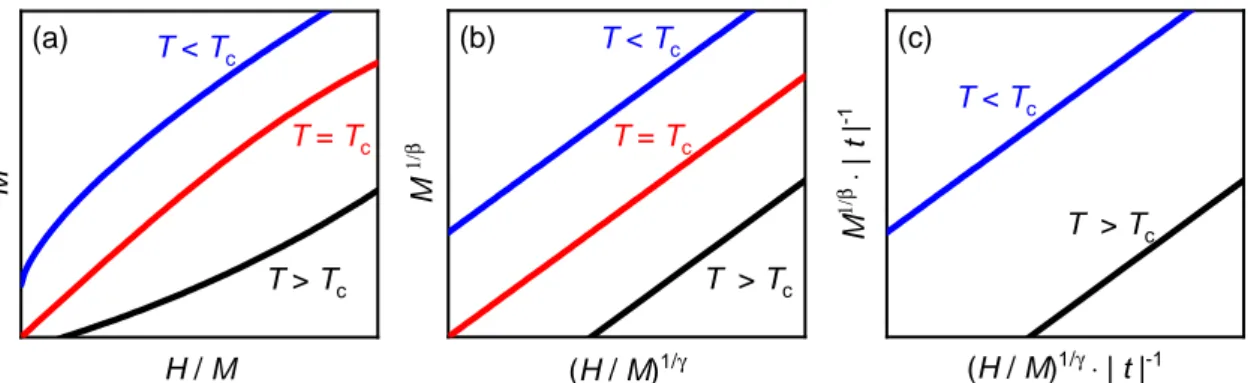
The Arrott plot is a special way of presenting magnetization measurements of a ferro-
magnet, see Fig. 2.3. If a material shows a second-order phase transition of Landau-type,
M 2 is linear in M/H in the vicinity of the transition temperature. The intercept of this
curve is temperature-dependent, i.e., positive for T < T C and negative for T > T C . Thus,
2.2 Magnetism
M 2
H / M T = T c
T > T c
T < T c
( a ) ( b )
M 1/ β ( H / M ) 1 / γ
T < T c
T = T c
T > T c
( c )
M 1/ β ⋅ | t | -1 ( H / M ) 1 / γ ⋅ | t | - 1
T < T c
T > T c
Figure 2.3 Arrot plots for magnetization measurements. The original Arrott plot (a) displays magnetization measurements for temperatures close to the ferromagnetic orde- ring temperature as M 2 vs. H/M. For a system that can be described with mean-field exponents, this yields a linear behavior around T C . (b) shows the modified Arrott plot, which takes critical fluctuations into account and allows to describe the critical behavior around T C for other universality classes. In the scaled Arrott plot (c), all temperatures collapse onto two different curves.
the critical temperature can be determined precisely by measuring the magnetization of a ferromagnet for di ff erent temperatures close to T C and using the Arrott plot scheme. Often, a material does not follow the mean-field theory, but critical fluctuations are dominating.
In this case, the Arrott plot does not yield straight lines due to changes of the critical expo- nents of the system. The modified Arrott plot, which relates M 1/β and (H/M) 1/γ , accounts for these changes. This allows an analysis of the criticality and the corresponding uni- versality class of the material. Magnetization curves for multiple temperatures follow a scaling relation and collapse onto two linear curves, see panel (c). 3
Antiferromagnetism
If the exchange constant J i j is positive, the involved magnetic moments favor an antipa- rallel alignment, see Eqn. (2.12). The corresponding long-range order is called antifer- romagnetic order. An antiferromagnet often consists of two sublattices of ferromagnetic moments whose magnetization is equally large but di ff ers in sign, which yields a van- ishing net magnetization without an external magnetic field. Above the critical ordering temperature T N , called Néel temperature, the susceptibility follows the Curie-Weiss law of Eqn. (2.13) but with a negative Curie-Weiss temperature θ. Below T N , the susceptibi- lity is anisotropic. For a magnetic field parallel to the ordered moments, the susceptibility approaches zero, while it remains constant for the perpendicular alignment.
3 Another way of checking the scaling behavior is by plotting M 2 (T/T C − 1) 1/β vs. H/M(T /T C − 1) 1/γ .
Frustration
Frustration in solid-state physics is known as the problem of competing interactions due to local (geometric) constraints. An elementary unit for frustration is a triangle, see Fig 2.4(a). The Ising spins on the edges of a triangle shall have a nearest-neighbor an- tiferromagnetic coupling. If one pair is aligned antiparallel, the third spin is frustrated since both orientations have the same energy and in any case one neighbor is oriented antiparallel, while the other is parallel. It cannot gain coupling energy with both nearest neighbors. In 1950, Wannier showed that this system does not order down to zero tempe- rature and possesses a degenerate ground state [45]. The ground state degeneracy grows exponentially with the number of spins that obey this frustration. Thus, e.g., the triangular lattice has a residual entropy violating the third law of thermodynamics, which demands a vanishing entropy as the temperature approaches 0 K. Further predictions and realizations of the triangular lattice will be discussed below.
Another example of frustration is the interplay of nearest neighbor (NN) and next- nearest neighbor (NNN) interaction on a chain, see Fig. 2.4(b). In such a chain with ferromagnetic or antiferromagnetic coupling J for the NN and antiferromagnetic NNN J 0 , not all couplings can be satisfied at once. The ground state of this system is the ↑↑↓↓ confi- guration if J 0 > |J| / 2 . For a system without Ising anisotropy, see Fig. 2.4(c), a cycloidal spin arrangement minimizes the energy for J 0 > |J| / 4 . The cycloid can break the inversion sym- metry, and, thus, it can lead to a polar structure. Via the inverse Dzyaloshinskii-Moriya in- teraction, which is mediated by spin-orbit coupling, a ferroelectric polarization can occur.
In such a system, the direction of the ferroelectric polarization is directly related to the handedness of the spin-cycloid, and, thus, a large magnetoelectric coupling is found. This type of coupled order is called multiferroicity.
J ' > 0 J < 0
J ' > |J|
4 J ' > 0
J < 0 J ' > |J|
2
(a) (b) (c)
Figure 2.4 Examples for geometrical frustration. (a) shows magnetic frustration on a
triangle with antiferromagnetic coupling. (b) and (c) show spin chains with ferromagne-
tic NN coupling J and antiferromagnetic NNN coupling J 0 . The chain in (b) has Ising
anisotropy and the ground state shows ↑↑↓↓ order for J 0 > |J| / 2 , while the chain in (c)
with isotropic Heisenberg spins and J 0 > |J| / 4 has a cycloidal ground state.
2.2 Magnetism
2.2.3 2D triangular lattice
The 2D triangular lattice with antiferromagnetic interaction is a highly-frustrated model system that has been studied extensively by di ff erent theoretical approaches. According to Mermin-Wagner theorem [46], it is impossible for any continuous symmetry to be broken spontaneously in a two-dimensional lattice at finite temperatures, and, thus, magnetic long- range order cannot emerge. There is the possibility of a quasi-long-range order through a topological phase transition, which is called (Berezinskii-) Kosterlitz-Thouless (BKT) transition. In such a transition, the correlation length diverges exponentially. Below the transition temperature, vortex-antivortex pairs are bound, while they are free above the transition [47].
For the spin- 1 / 2 Heisenberg antiferromagnet, it was shown that in the ground state neigh- boring moments form a relative angle of 120° [48]. This ground state has two possible chiralities, see Fig. 2.5(a). Without any anisotropy, the system still has a large degeneracy since the direction of the moments is not defined, but only their relative angle. This dege- neracy can also be broken by further neighbor interactions which then stabilize multiple fractional magnetization states with sublattice (SL) structures [49]. Besides the quantum- mechanical nature of the S = 1 / 2 moments, also the classical version hosts interesting phases at finite temperatures. In a magnetic field, see Fig. 2.5(b), Monte-Carlo simulations reveal three ordered phases [50]. Two temperature-driven phase transitions are found in small magnetic fields. The transition from the paramagnetic phase to the 2up-1dw phase with a 1 / 3 M sat magnetization is continuous, while the following transition to the ground state, the so-called Y phase, a canted version of the 120° state, is a BKT transition. In larger magnetic fields, a continuous phase transition into a canted 2up-1dw state is found.
The magnetic-field driven transition from the pure 2up-1dw to the canted version is an- other BKT transition and occurs at a field strength of ∼3J. Further studies take di ff erent perturbations into account. If there is an easy-axis anisotropy present, the 2up-1dw phase is stabilized further [51]. For a large anisotropy (D J), a zero-magnetization plateau was proposed up to magnetic fields of B c ∼ J
3/ D
2[52]. An infinite anisotropy Ising system was studied by Metcalf [53] and Tanaka and Uryû [54] who propose four possible ground states for the triangular lattice depending on the ratio of the NN and NNN interaction.
Any 3D crystal also has a finite interlayer coupling, that motivates studies of more com-
plex models in order to explain experimental results of materials, e.g., AgNiO 2 [55]. Such
models that also include further neighbor interactions with competing influence or aniso-
tropic exchange interactions, exhibit even more complicated magnetic field vs. temperature
phase diagrams [56, 57]. An exemplary phase diagram is shown in Fig. 2.5(c), which is
calculated for a system of triangular layers with NN coupling J 1 = 1, the NNN interaction
J
1= 1 J
2= 0.15 J = -0.15 D = 0.5
(a) (b) (c)
Figure 2.5 Magnetic structure and phase diagrams for triangular lattice models. (a) shows the two 120° ordered magnetic ground states of the S = 1 / 2 with di ff erent chirality.
The phase diagram of the classical spin model on a triangular lattice in a magnetic field (b) was adapted from Ref. [50]. (c) shows the phase diagram for a stacked triangular lattice with J 1 = 1, J 2 = 0.15, J ⊥ = −0.15, and D = 0.5 from Ref. [57]. The axes are measured in units of J 1 .
J 2 = 0.15, a ferromagnetic interlayer coupling J ⊥ = −0.15, and an easy-axis anisotropy D = 0.5 using the following Hamiltonian:
H = J 1 X
hi ji
1S i · S j + J 2 X
hi ji
2S i · S j + J ⊥
X
hi ji
⊥S i · S j − D X
i
(S z i ) 2 − h X
i
S z i .
The resulting phase diagram consists of six ordered phases below the ordering temperature of about 0.43J 1 . At zero temperature, three magnetization plateaus are found with values of 0, 1 / 3 M sat , and 1 / 2 M sat .
2.2.4 Hexagonal closed packed structure
The ABAB stacking of triangular layers yields the hexagonal closed packed (hcp) lattice.
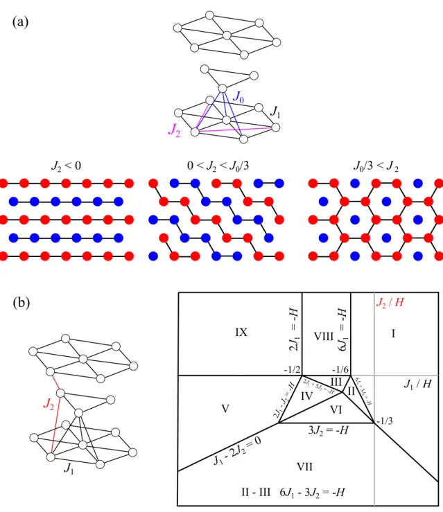
The magnetism of Ising moments on this lattice was studied with multiple techniques. In the following, two di ff erent approaches are presented, one numerical and one analytical.
The model of Matsubara and Inawashiro [58] takes three couplings into account, the out-
of-plane coupling J 0 and the in-plane NN and NNN couplings J 1 and J 2 , see Fig. 2.6(a). It
is further assumed that J 0 J 1 , which results in a quasi 2D system. Depending on the ratio
of J 0 and J 2 di ff erent ground state orderings are found by Monte-Carlo simulations. For
2.2 Magnetism
an antiferromagnetic J 2 , the ground state shows ferromagnetic stripes along one crystallo- graphic axes that are alternating in the other direction, see Fig. 2.6(a). This state of course occurs in three twin domains. In an intermediate range 0 < J 2 < J
0/ 3 , the ground state shows an antiferromagnetic arrangement in one direction, while the other two are ordered in an 2up-2dw manner. This state can equally be described by ferromagnetic zig-zag chains. In the case of J
0/ 3 < J 2 , the ground state has a net-magnetization of 1 / 3 M sat , resulting from a hexagonal arrangement of ferromagnetic spins with a centered antiferromagnetic spin.
A more general perspective was studied by Kudo and Katsura [59]. They evaluated the
phase diagram for the hcp lattice with Ising moments including NN and NNN interaction
(J 1 and J 2 ) with an analytical approach. Additionally, their model captures the influence
of a magnetic field. The obtained J 1 -J 2 -H phase diagram is shown in Fig. 2.6(b). In total,
they find nine ordered phases and show the corresponding magnetic structures. In zero-
field, the phases VII, V, and IX correspond to a more or less complex antiferromagnetic
ground state with a vanishing magnetization, while phase I reflects the (fully polarized)
ferromagnetic ground state. By applying a magnetic field, numerous phase transitions
occur, depending on the ratio of J 1 and J 2 . Up to four phase transitions into the finally
fully polarized phase are possible. Some of these intermediate phases exhibit a fractional
magnetization. Phases IV and VI obey 1 / 3 M sat , III and VIII 1 / 2 M sat , and II 2 / 3 M sat . Further
studies of the magnetic order on the hcp lattice with further neighbor interactions do not
take magnetic-field influences into account [60, 61].
(a)
(b)
J 2 < 0 0 < J 2 < J 0 /3 J 0 /3 < J 2
J 1
J 2
J 1 J 0
J 2
IX VIII I
VII
V IV
VI III II
J 2 / H
J 1 / H
J 1 - 2 J 2 = 0
-1/3 -1/6
-1/2
2 J -
1J
2= - H
3J 2 = -H
2 J 1 = - H 6 J 1 = - H
6J1 + 3
J2 = - H 2J1 + 5J2 = -H
II - III 6J 1 - 3J 2 = -H
Figure 2.6 Magnetic structures and phase diagrams of Ising moments on the hcp lattice
with different exchange couplings. The model of (a) includes the in-plane NN and NNN
interactions J 1 and J 2 and the NN interlayer coupling J 0 [58]. Furthermore, J 0 J 1
is assumed. There are three di ff erent ground states depending on the ratio of J 0 and J 2 .
The model in (b) uses Ising moments connected via the NN interaction J 1 and the NNN
interaction J 2 . The corresponding rich J 1 -J 2 phase diagram in a magnetic field is adapted
from Ref. [59].
3 Experimental
Contents
3.1 Cryogenic setups . . . . 26 3.2 Magnetic field . . . . 27 3.3 Magnetization . . . . 28 3.3.1 SQUID magnetometer . . . . 28 3.3.2 Pick-up techniques . . . . 29 3.3.3 Faraday magnetometer . . . . 30 3.4 Thermal expansion and magnetostriction . . . . 36 3.5 Specific heat and magnetocaloric e ff ect . . . . 39 3.6 Pyrocurrent . . . . 44 3.7 Electric transport properties . . . . 45 The experimental investigations of this work study thermodynamic and transport pro- perties under extreme conditions, namely at low temperature and in strong magnetic fields.
This requires di ff erent cryogenic setups and magnets. The following quantities are studied:
magnetization, thermal expansion, magnetostriction, specific heat, dielectric polarization,
and electric dc transport. The relevant experimental fundamentals and important details
about the used setups are presented in the following. Hereby, a focus is put on magnetiza-
tion measurements as it is essential to explore the magnetism of any magnetic material for
a general understanding and also a basic characterization. In the scope of this thesis, mul-
tiple standard techniques were used to characterize materials in di ff erent temperature and
magnetic-field ranges. Additionally, a new magnet was set up to improve the resolution of
the Faraday magnetometer. The developed principle is explained in detail.
3.1 Cryogenic setups
In general, liquid helium is used to provide the cooling power for low-temperature measu- rements. With a variable temperature insert (VTI) for a 4 He bath cryostat and a Physical Property Measurement system (PPMS, Quantum Design) it is possible to cover the tem- perature range from 1.8 K to 400 K. For the PPMS, there are multiple options available that allow to measure, e.g., specific heat, magnetization, and resistivity easily and with a good reproducibility. Nonetheless, each option of this commercial equipment itself lacks in terms of versatility. All options function automated with only little possibilities for ma- nual user optimization. In addition to the PPMS, the VTI allows for custom probes, e.g., a dilatometer to measure the thermal expansion of a sample. Information about the VTI can be found in Ref. [62]. Furthermore, evacuated dipsticks were used for measurements in the range from 7 K to 300 K. The temperature is controlled via a manganin wire heater wound around a beaker that covers the sample space and which is controlled by a Lake- shore 340 temperature controller. Such dipsticks have very good temperature stability.
Further information about the systems can be found in Refs. [63, 64].
To reach temperatures below 1.8 K, a 3 He cooling unit is required. The HelioxVL probe (Oxford Instruments), see Fig. 3.1 is operated in a bath cryostat and reaches temperatures down to 250 mK. Custom sample holders allow an extensive pool of measurement tech- niques. The HelioxVL is inserted into a 4 He bath dewar through a sliding seal. The first cooling stage is the so-called 1-K pot or λ plate. The vapor pressure of Helium is reduced via a needle valve to about 20 mbar and, thus, the 1-K pot is cooled down to 1.8 K. At this temperature, gaseous 3 He in a closed system condenses and gathers at the bottom of the HelioxVL in the 3 He pot. Via pumping on this 3 He bath, it is possible to reach the base temperature of about 250 mK. The pumping is performed by an active-coal sorb that acts as a cryo pump. The cooling power ends once all the liquid 3 He is evaporated, which happens after about 20 h at base temperature. Afterwards, the 3 He sorb has to be heated to about 30 K, so that the adsorbed gas degases. Then, it can reliquify at the λ plate.
This process is called regeneration or recondensation. Within this process, the sample temperature increases to about 2 K. The base temperature is restored by cooling the sorb.
For measurements at temperatures that di ff er from the base temperature, two di ff erent heaters are used. Below 2 K, the cooling power is controlled by the vapor pressure of the
3 He via the temperature of the cryo-pump sorb. Above 2 K, the 3 He pot is heated directly so
that temperature control is possible up to 50 K. The temperature stability strongly depends
on the absolute temperature. The temperature control is poor close to 2 K when switching
between the two heaters. Therefore, stabilized temperatures and especially heating ramps
3.2 Magnetic field
sliding seal
3
He Pot
conical seal
3
He sorbtion pump
3
He reservoir pumping lines vacuum feedthrough,
e.g., coaxial cables
needle valve stepper motor
4
![Figure 4.8 Comparison of the criticality study to the work of Snyder from Ref. [114].](https://thumb-eu.123doks.com/thumbv2/1library_info/3698191.1505900/67.892.133.722.322.719/figure-comparison-criticality-study-work-snyder-ref.webp)
![Figure 4.9 Magnetization measurements M(H) at 2 K for the high-symmetry directions [1 0 1] c (a) and [0 1 0] c (b)](https://thumb-eu.123doks.com/thumbv2/1library_info/3698191.1505900/69.892.115.744.166.420/figure-magnetization-measurements-m-h-high-symmetry-directions.webp)