A Probe of Zigzag Edge Magnetization

(1)

A Probe of Zigzag Edge Magnetization

Jan Bundesmann,¹ Ming-Hao Liu (劉明豪),¹ ˙Inan¸c Adagideli,² and Klaus Richter¹

1Institut f¨ur Theoretische Physik, Universit¨at Regensburg, 93040 Regensburg, Germany

2Faculty of Engineering and Natural Sciences, Sabanci University, 34956 Orhanli-Tuzla, Istanbul, Turkey

We investigate spin transport in diffusive graphene nanoribbons with both clean and rough zigzag edges, and long-range potential fluctuations. The long-range fields along the ribbon edges cause the local doping to come close to the charge neutrality point formingp-n junctions with localized magnetic moments, similar to the predicted magnetic edge of clean zigzag graphene nanoribbons.

The resulting random edge magnetization polarizes charge currents and causes sample-to-sample fluctuations of the spin currents obeying universal predictions. We show furthermore that, although the average spin conductance vanishes, an applied transverse in-plane electric field can generate a finite spin conductance. A similar effect can also be achieved by aligning the edge magnetic moments through an external magnetic field.

PACS numbers: 73.23.-b 72.25.-b 72.80.Vp

I. INTRODUCTION

Understanding graphene edges is of profound interest for the investigation of graphene nanostructures as the edges induce peculiar features depending on the edge orientation, that strongly influence the electronic prop- erties of graphene. Armchair nanoribbons can be ei- ther metallic or semiconducting depending on the ribbon width while zigzag (zz) nanoribbons are always metallic due to the presence of a state localized at the edge^1,2. Moreover thezzedges are predicted to be magnetic at half filling, with oppositely spin-polarized edges, based on the mean-field approximation of the Hubbard¹ and the extended Hubbard model³. Density functional theory (DFT) calculations^4–7, exact diagonalization and quantum Monte Carlo simulations⁸, as well as diagram- matic perturbation theory⁹, produced results affirming thezz edge magnetization. On the other hand the sta- bility of the edge state (and consequently its magnetization) has been doubted, as it should only exist for edges passivated with a single hydrogen atom and, moreover, the magnetic ordering should only be observable under “ultraclean, low-temperature conditions in defect- free samples”¹⁰. For a recent review see Ref. 11.

On the experimental side, scanning tunneling mi- croscopy (STM) measurements indeed confirmed the presence of an increased local density of states at zz edges^12–14. The measurements, however, were not spin sensitive. While there is evidence of magnetism in graphene^15–17, its origin might also be adatoms and impurities in addition to magneticzzedges.

Theoretical studies already suggested measuring spin transport as a probe of edge magnetism^18,19. However, it was unclear whether the predictions, which assumed ribbons close to half-filling, were directly applicable to experiments where both edge roughness and disorder could potentially mask the effect of edge magnetism. In this work, we show that disordered graphene nanoribbons exhibit universal spin conductance fluctuations due to edge-

magnetism. Moreover, the spin conductance fluctuations remain finite in a large energy interval as long as potential disorder induces charge neutrality at the edges. Further- more, we propose how to control the spin conductance electrically.

II. MODEL

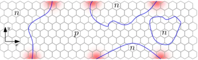
In realistic systems, long-range potential fluctuations generate lines of local charge neutrality. We assume that magnetic clusters form where these lines and zz edges coincide; see Fig. 1. In order to check this assumption, we self-consistently calculated the mean-field Hubbard Hamiltonian for simple systems with non-constant potential and found that local magnetic moments indeed formed at zz edges near charge-neutrality points. Further sources of magnetic moments in graphene were ignored.

Defects or non-magnetic adatoms could, possibly, also induce magnetism in graphene close to charge-neutrality.

The probability of a point-like defect coinciding with local charge neutrality in a disordered systems is, however, small compared to the probability of a sequence of edge atoms with a local potentential close to charge-neutrality.

We considered systems free of magnetic impurities as their deposition, nowadays, is well controlled²⁰. We now consider spin-dependent quantum transport through dis-

n n

n p

x y

n

FIG. 1. Formation of local zigzag edge magnetic moments.

Whenever isopotential lines (blue) separatingn-doped from p-doped regions hit an edge, a finite magnetization is locally assumed (red).

arXiv:1305.6792v2 [cond-mat.mes-hall] 28 Mar 2014

(2)

orderedzznanoribbons and analyze imprints of localzz edge magnetism in the spin conductance for various sce- narios of the relative orientation of the magnetic clusters.

We use a tight-binding description of graphene, H=X

i,s

V(~ri)c^†_i,sci,s+X

i,j,s

ti,jc^†_i,scj,s

+X

i,s,s⁰

c^†_i,s(m~i·~σ)s,s⁰ci,s⁰, (1) where the sums run over atomic sites (iandj) and spin indices (sand s⁰). Hereti,j =t if the atomsiandj are nearest neighbors andti,j=t⁰for next-nearest neighbors.

~σ= (σx, σy, σz) is the vector of Pauli matrices in real spin space, thus the third term in Eq. (1) acts like a Zeeman term.

We now specify our model. To model long range disorder that may originate from, say, charges trapped in the substrate, we shall adopt a smooth static disorder potential, given by

V(~r) =X

n

Vnexp

−|~r−~rn|² 2σ_dis²

, (2)

that is characterized by a random disorder strengthVn ∈ [−Vdis, Vdis] and a correlation lengthσdis.

Owing to the potential fluctuations we assume the magnetization to be finite only nearp-n junctions close to the edge²¹. The magnetization is further assumed to decay with distancedfrom the p-njunction at the edge as a Gaussian, exp(−d²/d²₀), where d0 is a phenomenological decay length. Several magnetic clusters will form along the edges; see Fig. 1. Within these clusters the

0.0 0.1 0.2 0.3 0.4 0.5 0.6 0.7

hGi,hGSi (a)

−0.5 0.0 0.5 E[eV]

0.00 0.02 0.04 0.06 0.08 0.10 0.12 0.14 0.16

VarG,VarGS (c)

(b)

−0.5 0.0 0.5 E[eV]

(d)

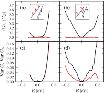
FIG. 2. Energy dependence of average conductance hGi (black) in units ofe²/hand spin conductancehGSi (red) in units of _4π^e for (a) modelaand (b) modelb(see text). Corre- sponding variance of charge and spin conductance for model a (c) andb (d).

magnetization has opposite sign for sublatticeA andB, but the net magnetization is nevertheless finite.

We consider three models in this paper how the different clusters relatively align; see also the insets in Figs.2 and3.

a. Fully Aligned Moments. This configuration is an extension of the simple model of constant magnetization along a ribbon’s edge which has been used before to model transport in graphene^4,5. If the magnetic clus- ter formed at an edge segment is mainly composed of atoms of sublatticeA (B) its net magnetization points upwards (downwards).

b. Uncorrelated Moments. The mean-field description used to derive the antiferromagnetic alignment of the sublattices of graphene is not able to determine a preferred axis along which the electrons’ spins align. Mag- netic moments at different p-n junctions need not be aligned nor collinear. Thus it is a natural and realistic extension of modela to assign a random direction to the magnetization at eachp-njunction.

c. Ferromagnetic ordering of the edges. This model is similar to modela. The clusters, however, get assigned a direction that additionally depends on the edge they are lying on. Clusters with mainly edge atoms of sublattice A(B) point upwards (downwards) on the left edge and downwards (upwards) on the right edge. Formally the Hubbard model allows for this solution as shown for clean zznanoribbons (cf. Fig. 4 in Ref. 22). This phase might be triggered by applying small magnetic field.

−0.6

−0.4

−0.2 0.0 0.2 0.4 0.6 0.8

hGi,hGSi (a)

−0.5 0.0 0.5 E[eV]

0.00 0.05 0.10 0.15

VarG,VarGS (c)

(b)

−0.5 0.0 0.5 E[eV]

(d)

FIG. 3. hGi(black) in units ofe²/handhGSi(red) in units of e/4π as a function of energy E for (a) ferromagnetically aligned magnetic clusters in a rather clean ribbon according to model c and (b) when edge disorder randomizes the A andB sublattice segments and thus the sign of the magnetic moments. (c, d) Corresponding variance ofGandGS.

(3)

III. TRANSPORT CALCULATIONS We model transport through graphene nanoribbons in the presence of random long-range disorder [Eq. (2)] with Vdis = 300meV, σdis ≈ 1nm. For modelb, also the orientation of the magnetic moments at differentp-njunctions is randomized. Both, nanoribbons with smooth and rough edges were considered. Edge disorder is created by iterating over the edge atoms and removing them with a probability of 2% for this work. This procedure was re- peated up to ten times to increase edge disorder and to extend the size of edge defects. An example is shown in the inset of Fig. 5. The edge disorder acts as an additional source of momentum scattering. It also randomizes the magnetic moments along an edge. Hence, model a and c become very similar in the presence of edge disorder; see inset between Figs.3(b) and (d). Spin- dependent quantum transport is simulated by means of a recursive Green’s function method²³. The considered ribbons are 40 - 50nm wide and 500nm - 1µm long. With these parameters transport takes place mainly in the localized regime. We calculate spin-resolved transmission probabilities, the transmission matrix in real spin space becomes

T =

T↑↑ T↑↓

T↓↑ T↓↓

. (3)

The charge conductance is the sum of all four probabilities, G = ^e_h²(T↑↑+T↑↓+T↓↑+T↓↓), subtracting transmission to spin down from transmission to spin up, Gs= _4π^e (T↑↑+T↑↓−T↓↑−T↓↓), yields the spin conductance.

A. Average spin conductance

Without external fields (modelsaandb) total average charge conductancehGiincreases with distance from the CNP, while the average spin conductance hGSi is suppressed; see Figs.2(a, b). In the modelaof fully aligned moments, we find that the sample-to-sample fluctuations of G andGS, i.e. VarG and VarGS, coincide; see Fig.

2(c). For model b (uncorrelated random directions of magnetic moments) hGSi = 0 as expected, but notably the variance is finite; see Fig.2(d). Var(GS) differs, however, from Var(G) due to off-diagonal couplings in the transmission matrix (3) in this case.

As shown in Fig.3(a), carrying out the transport sim- ulation with ferromagnetically ordered edges (model c) yields finite average spin conductance which is positive for positive Fermi energy and vice versa. The extrema of GSlie at a distance away from the CNP that is consistent with the positions of the spin-split edge states which are not spin-degenerate any more.

In order to understand the results presented in Figs.

2 and 3, we consider a simple model in which we assume the magnetic clusters to act as spin filters with a

10⁻¹ 10⁰

ξ/L 10¹

10²

Var(lnG),Var(ln|GS|)

G G_S

10⁻¹ 10⁰

ξ/L 10⁰

10¹

−hln|GS|i

FIG. 4. Var[lnG] forGin units of ^e_h² (black) and Var[lnGS] for GS in units of _4π^e (red) as a function of ξ/L for various ribbons of length L and localization lengthξand random magnetic moment orientation, modelb. In the inset the loga- rithm of the absolute value of the spin conductance is plotted as a function ofξ/Lfor the same ribbons. The blue lines are the values expected from DMPK equation²⁵, see text.

preferred direction depending on the orientation of the localized magnetic moment. For a given ribbon we then calculate the number ofp-njunctions with positive (N↑) or negative (N↓) orientation, as well as their difference

∆ =N↑−N↓, which is proportional to the ribbon’s total magnetization²⁴. For models a and b,h∆i= 0, and hence the average magnetization is zero, resulting in a suppressed average spin transmission. In modelc, however, ∆ is finite leading to finite average spin conductance. The spin-polarized states are shifted away from the CNP by a value corresponding to the peak strength of the local magnetization²². This is where spin polariza- tion is most efficient leading to the extrema of the spin conductance.

Within all models, edge disorder can lead to a random- ization of the magnetic moments along the edges. The effect is negligible for model a and b, where h∆i = 0.

In modelc it leads to decreasing and eventually vanish- ing ∆. We find that the average spin conductance also vanishes in agreement with our model; see Fig.3(b).

B. Universal spin conductance fluctuations An instrument to retrieve general information about mesoscopic systems are conductance fluctuations which, according to random matrix theory, are independent of the particular considered system²⁶. In graphene, they can, e.g., indicate the symmetry class and system degeneracies^27–29 or be used to extract the phase coherence time³⁰. Here we focus on sample-to-sample fluctuations. For strongly localized mesoscopic systems the conductance shows a log-normal distribution²⁶. The cal-

(4)

culation of the exact distribution of lnG for a disordered system is obtained by solving the Dorokhov-Mello- Pereyra-Kumar (DMPK) equations^31,32. For the dimen- sionless conductance,G/G0, withG0=e²/h, this yields

−hlnG/G0i = ¹₂Var(lnG/G0) = 2L/ξ for systems of lengthL and localization lengthξ²⁵. This prediction is approximately fulfilled for the charge conductance in our simulated ribbons; see black curve in Fig.4.

The spin conductance has to be studied via its absolute value. It turns out that, for different systems, mean and variance of ln|GS/(_4πê)|follow a universal curve as a function of ξ/L independent of the exact choice of the phenomenological parameters describing the local magnetization. For the aligned magnetic moments (model a) Var(ln|GS/(_4πê)|) obeys the same relation as Var[ln(G/G0)] which is an indication that spin-up and -down channel are uncorrelated. In Fig. 4 it can be seen that also for model b, uncorrelated magnetic moments, Var(ln|GS/(_4πê)|) follows the same universal law as Var[ln(G/G0)]. For modelb,−hln|GS/(_4πê)|iis larger than the universal value from DMPK equation; see inset of Fig. 4. This is a result of the projection of the three dimensional spin expectation value onto thez axis. For modela such a deviation is not found.

C. Effect of a transverse in-plane electric field For pristine graphene it has been predicted that the application of a transverse in-plane electric field greater than a certain threshold turns a graphenezzribbon into an insulator for one spin direction and into a metallic phase for the other one⁴. We now show how an electric field can lead to finite spin conductance in disordered graphene nanoribbons without a threshold for the electric field. Therefor, we investigate model a again in the presence of a potentialVtilt increasing linearly across the ribbon from−V0/2 on the left edge to +V0/2 on the right edge, which can be viewed as arising from the application of a transverse in-plane electric field.

The obvious effect of a transverse potential drop is a change in the number ofp-njunctions. For modelawith- out edge disorder this leads to an imbalance between the number ofp-njunctions on opposite edges and, thereby, directly to the difference ∆ =N↑−N↓between localized magnetic moments pointing upwards and downwards. As mentioned above, ∆ 6= 0 leads to a finite spin conductance. A corresponding example is shown in Fig.5. For these calculations magnetization does not exceed 0.01t and decays rather fast,d0= 0.25nm.

In model a the transmission as a function of ribbon lengthL, Eq. (3), is fully defined by two scaling parameters L/ξ↑ and L/ξ↓ for the two spin blocks: T↑↑/↓↓ = exp(−L/ξ↑/↓), leading to transmission T = T↑↑+T↓↓

and spin transmission TS = T↑↑−T↓↓, respectively³³. The scaling parameter for each spin block, L/ξ↑/↓, depends both on energy and ∆. To leading order the in- verse normalized localization length for each spin block

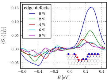
FIG. 5. Average spin conductance of nanoribbons under the influence of a transverse in-plane electric field. The potential difference leads to a maximum spin conductance at Fermi energiesVdis−t⁰ and −Vdis. Different curves showhGSi for increasing edge disorder, from perfectly clean zz edges, to edges with approximately 8% defects. The inset visualizes how spins align along a defective edge piece with blue (red) circles indicating positive (negative) magnetized atoms. The size of the circles is proportional to the local magnetization.

is assumed to depend linearly on ∆,L/ξ↑/↓=L/ξ0±γ∆, as confirmed by our numerical data. This impliesTS ≈ 2γ∆ exp(−L/ξ0). Hence, the positions of the extrema of TS(E) are given by the peaks of ∆(E). For clean zigzag ribbons ∆ is given by the difference of magnetic clusters along left and right edge. We assume the local Fermi level for a given transverse coordinateyto exhibit a Gaussian distribution aroundEF−Vtilt(y) given by the global Fermi levelEF and the value of the transverse potential drop Vtilt at position y. The distribution width σE is given by the strength of the long range potential disorder σE ∝Vdis. Then, the number of p-n junctions can be estimated from the energy distribution along the two edges,ρleft/right, and consequently ∆(E),

∆(E)∝ Z 0

−t⁰

(ρright(E)−ρleft(E))dE. (4)

∆(E) is peaked around ±σE as long as Vtilt < σE and around ±Vtilt otherwise. The numerical results shown in Fig.5 follow this prediction. Notably, if we sharpen the distribution of the local Fermi level by decreasing the disorder strength we eventually recover, as a limiting case, the mechanism of half-metallicity presented in Ref.

4.

Edge disorder is expected to reduce ∆(E) by random- izing the spin orientation along the edges. To investigate this effect we simulated transport through nanoribbons at different edge defect rates; see Fig.5. Apparently the spin conductance decreases with increasing edge disorder and tends to zero for a defect rate of about 10%.

While the above proposal could open a route to an

(5)

all-electric spin current creation and control in graphene, as spin transport experiments are nowadays performed with high accuracy^34,35, it represents also a generic way of detecting edge magnetization.

IV. SUMMARY

In conclusion, we considered spin-dependent electron transport in graphene nanoribbons. We showed that even in the diffusive case and for random edge magnetic moments finite spin conductance fluctuations persist follow- ing universal predictions. Finite spin conductance fluctuations are visible within a large energy range, demon-

strating how potential fluctuations help observing edge magnetism in graphene. Aligning the localized magnetic moments can lead to finite average spin conductance.

Furthermore we showed that the application of a transverse in-plane electrical field can be used to detect edge magnetism and to polarize spin transport in graphene.

V. ACKNOWLEDGEMENTS

We gratefully acknowledge Deutsche Forschungsge- meinschaft (within SFB 689) (J.B. and K.R.), Alexan- der von Humboldt Foundation (M.H.L.) and the funds of the Erdal ˙In¨on¨u chair (˙I.A.) for financial support. ˙I.A.

thanks University of Regensburg for their hospitality.

1 M. Fujita, K. Wakabayashi, K. Nakada, and K. Kusakabe, J. Phys. Soc. Jpn.65, 1920 (1996).

2 K. Nakada, M. Fujita, G. Dresselhaus, and M. S. Dressel- haus, Phys. Rev. B54, 17954 (1996).

3 A. Yamashiro, Y. Shimoi, K. Harigaya, and K. Wak- abayashi, Phys. Rev. B68, 193410 (2003).

4 Y.-W. Son, M. L. Cohen, and S. G. Louie, Nature444, 347 (2006).

5 M. Wimmer, I. Adagideli, S. Berber, D. Tom´anek, and K. Richter, Phys. Rev. Lett.100, 177207 (2008).

6 W. L. Wang, O. V. Yazyev, S. Meng, and E. Kaxiras, Phys. Rev. Lett.102, 157201 (2009).

7 T. O. Wehling, E. S¸a¸sıo˘glu, C. Friedrich, A. I. Lichtenstein, M. I. Katsnelson, and S. Bl¨ugel, Phys. Rev. Lett. 106, 236805 (2011).

8 H. Feldner, Z. Y. Meng, A. Honecker, D. Cabra, S. Wessel, and F. F. Assaad, Phys. Rev. B81, 115416 (2010).

9 H. Karimi and I. Affleck, Phys. Rev. B86, 115446 (2012).

10 J. Kunstmann, C. ¨Ozdo˘gan, A. Quandt, and H. Fehske, Phys. Rev. B83, 045414 (2011).

11 O. V. Yazyev, Rep. Prog. Phys.73, 056501 (2010).

12 Y. Kobayashi, K. Fukui, T. Enoki, and K. Kusakabe, Phys. Rev. B73, 125415 (2006).

13 K. A. Ritter and J. W. Lyding, Nat. Mater.8, 235 (2009).

14 X. Zhang, O. V. Yazyev, J. Feng, L. Xie, C. Tao, Y.-C.

Chen, L. Jiao, Z. Pedramrazi, A. Zettl, S. G. Louie, H. Dai, and M. F. Crommie, ACS Nano7, 198 (2013).

15 H. S. S. Ramakrishna Matte, K. S. Subrahmanyam, and C. N. R. Rao, The Journal of Physical Chemistry C113, 9982 (2009).

16 V. L. J. Joly, M. Kiguchi, S.-J. Hao, K. Takai, T. Enoki, R. Sumii, K. Amemiya, H. Muramatsu, T. Hayashi, Y. A. Kim, M. Endo, J. Campos-Delgado, F. L´opez-Ur´ıas, A. Botello-M´endez, H. Terrones, M. Terrones, and M. S.

Dresselhaus, Phys. Rev. B81, 245428 (2010).

17 R. R. Nair, M. Sepioni, I.-L. Tsai, O. Lehtinen, J. Keinonen, A. V. Krasheninnikov, T. Thomson, A. K.

Geim, and I. V. Grigorieva, Nature Phys.8, 199 (2012).

18 E. Grichuk and E. Manykin, JETP Letters93, 372 (2011).

19 R. Farghadan and E. Saievar-Iranizad, Journal of Applied Physics111, 014304 (2012).

20 K. M. McCreary, A. G. Swartz, W. Han, J. Fabian, and R. K. Kawakami, Phys. Rev. Lett.109, 186604 (2012).

21 Ap-njunction, in this context, is given when the local potential fulfills −t⁰ ≤E−V(~r) ≤0. These are the points where an increased local density of states exists similar to the zz edge state, which then according to the Hub- bard model leads to an ordered phase. We also assume the atomic chain to have a minimum length of 3 atoms that an edge state is formed according to Ref.2.

22 J. Jung and A. H. MacDonald, Phys. Rev. B 79, 235433 (2009).

23 M. Wimmer and K. Richter, J. Comput. Phys.228, 8548 (2009).

24 In fact we would have to consider the full three-dimensional magnetization for model b. For the sake of simplicity we restrict ourselves to the distinction between spin-up and -down.

25 J.-L. Pichard, inQuantum Coherence in Mesoscopic Sys- tems, NATO ASI Series B, Vol. 254, edited by B. Kramer (1991) p. p. 369, p. 369.

26 C. W. J. Beenakker, Rev. Mod. Phys.69, 731 (1997).

27 E. McCann, K. Kechedzhi, V. I. Fal’ko, H. Suzuura, T. Ando, and B. L. Altshuler, Phys. Rev. Lett.97, 146805 (2006).

28 M. Y. Kharitonov and K. B. Efetov, Phys. Rev. B 78, 033404 (2008).

29 J. Wurm, A. Rycerz, I. Adagideli, M. Wimmer, K. Richter, and H. U. Baranger, Phys. Rev. Lett.102, 056806 (2009).

30 S. Minke, J. Bundesmann, D. Weiss, and J. Eroms, Phys.

Rev. B86, 155403 (2012).

31 O. Dorokhov, JETP Lett.36, 318 (1982).

32 P. Mello, P. Pereyra, and N. Kumar, Ann. Phys.181, 290 (1988).

33 Spin flip is suppressed in modela.

34 N. Tombros, C. Jozsa, M. Popinciuc, H. T. Jonkman, and B. J. van Wees, Nature448, 571 (2007).

35 W. Han, K. McCreary, K. Pi, W. Wang, Y. Li, H. Wen, J. Chen, and R. Kawakami, Journal of Magnetism and Magnetic Materials324, 369 (2012).