Transport properties of superconducting and ferromagnetic hybrid structures

(1)

Transport properties of

superconducting and ferromagnetic hybrid structures

DISSERTATION ZUR ERLANGUNG DES DOKTORGRADES DER NATURWISSENSCHAFTEN (DR. RER. NAT.) DER FAKULT ¨AT F ¨UR

PHYSIK DER UNIVERSIT ¨AT REGENSBURG

vorgelegt von Sebastian Pfaller aus

Eichst¨ att

im Jahr 2015

(2)

(3)

Promotionsgesuch eingereicht am 16.12.2014

Die Arbeit wurde angeleitet von Prof. Dr. Milena Grifoni Pr¨ufungsausschuss:

Vorsitzender: Prof. Sergey Ganichev 1. Gutachter: Prof. Milena Grifoni 2. Gutachter: Prof. Christoph Strunk weiterer Pr¨ufer: Prof. Jaroslav Fabian Termin Promotionskolloquium: 22.10.2015

(4)

(5)

Introduction

Figure 1.: Conductance as a function of the gate voltage for two metallic islands with the same width, but different length. The island of the left panel is larger than the one of the right panel. Consequently the charging energy corresponding to the device of the left panel is smaller, leading to a shorter distance of the conductance peaks. Reprinted figure with permission from [1]. Copyright (1992) by the American Physical Society.

The discovery of the Coulomb blockade effect in the 1990’s triggered the field of electron transport in nanoscale devices. For the first time it was possible to reduce their dimensions to a point where charging effects of single electrons are dominating the transport behavior. In other words, with these devices it is possible to control electronically the tunneling of a single charge. Benefited by its potential applications in spintronics and quantum information processing the field evolved rapidly, and still does.

The first devices were metallic islands electrostatically defined in two dimensional electron gases (2DEGs) realized in semiconductor heterostructures.[1, 2, 3] A process involving the tunneling of an additional electron on the island requires a certain charging energy, which must be paid by externally applied bias and gate voltages.

In case they are not compensating the energy cost, no current can flow across the junction, prevented by the Coulomb blockade effect. A typical fingerprint of this effect are regular conductance peaks with a period proportional to the charging

(10)

Figure 2.: Differential conductance as a function of the gate and bias voltage of a carbon nanotube quantum dot coupled to two superconducting leads. Reprinted figure with permission from [20]. Copyright (2009) by the American Physical Society.

energy. They are found at the charge degeneracy points, separating voltage regions with a fixed number of particles. An example of these Coulomb oscillations is shown in Fig. 1, where the conductance is measured as a function of the gate voltage for two distinct devices.[1] They differ only in their length, while their width is kept constant. Correspondingly, the two samples have different charging energies, which are inverse proportional to the devices length. Therefore, the larger island (sample 2) has a shorter Coulomb oscillations period than the smaller one (sample 3).[1]

Besides the quantization of the electronic charge, the phenomenon can be described as purely classical. However, reducing further the dimensions of the devices one obtains a so called quantum dot. Now, the quantization of the electronic levels becomes visible, and quantum effects play a central role in the interpretation of the measurements. Besides quantum dots in semiconductor heterostructures,[3] they were also realized in carbon nanotubes [4, 5, 6, 7, 8, 9, 10, 11], semiconducting nanowires [12, 13, 14, 15], metallic nanoparticles [16], single fullerene molecules [17], self-assembled nanocrystals [18] and graphene quantum dots [19], to mention only a few.

Moreover, technological advances made it possible to connect these nanoscale devices to a wide variety of contact materials. Of particular interest are hybrid systems, where the leads significantly influence the transport characteristic of the device. Among the most interesting are, on the one hand, contacts with reduced dimensionality, like for example one dimensional carbon nanotubes,[21, 22] or two dimensional graphene,[23, 24, 19] or, on the other hand, contacts with strong electronic correlations, like superconductors[25, 26] or ferromagnets.[27] Due to the continuous improvement of fabrication techniques, it is possible to virtually elimi- nate most of the impurities and dirt in the devices. Together with a precise control of the relevant transport parameters, this allows to test theoretical predictions with a remarkable precision.

(11)

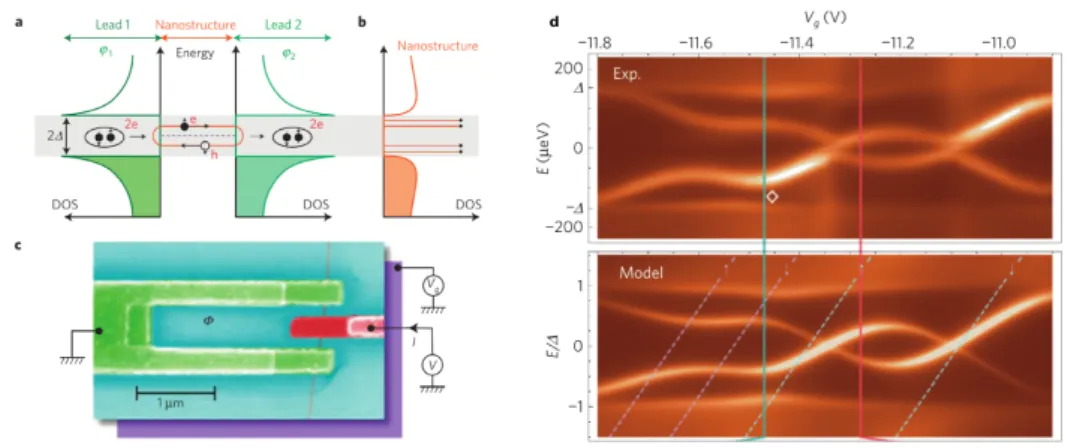
Figure 3.: a Schematic showing an Andreev bound state (ABS) in a nanostructure between two superconducting leads, which have a density of states (DOS) with a gap 2∆. In the subgap region (gray band) Andreev bound states are forming due to the Andreev reflection process, where an electron (e) is reflected as a hole (h)–its time-reversed particle—and vice versa. ABS are discrete resonant states of entangled electron-hole pairs confined between the superconductors. b) Local DOS of the carbon nanotube. c) Electron micrograph of the device. d) Experimental deconvolved density of states as a function of the gate voltage Vg and predictions of a double-quantum-dot model, at phase φ = 0. Reprinted by permission from Macmillan Publishers Ltd: Nat. Phys. [10], copyright (2010)

A huge interest in spin polarized transport in nanoscopic ferromagnetic hybrid systems, was initiated by the discovery of the giant magnetoresistance (GMR) effect in 1988 in artificially layered metallic structures, where non magnetic layers separate 3d ferromagnetic films.[28, 29] Their resistance crucially depends on the magnetic configuration of the layers, and it drops by changing from a parallel to an antiparal- lel alignment.[28, 29, 30] Due to the possibility of controlling the transport behavior of electronic devices by manipulating the additional spin degree of freedom, they have many applications in spin based electronics, known as spintronics.[31] With the effort of further reducing the dimensions of spintronic devices, ferromagnetic hybrid systems, where nanostructures are tunnel coupled to two ferromagnetic contacts, become interesting.[32, 27] As in the case of the GMR, the tunnel magnetoresistance (TMR) depends also on the relative alignment of the magnetization direction of the leads. [27] For nanostructures consisting of a tunnel coupled quantum dot molecule or metallic island, the spin polarized transport is not only influenced by the magnetization of the leads, but also by intrinsic interactions of the nanostructure, and the dominant Coulomb blockade effect.

Superconducting hybrid systems, on the other hand, are ideal to investigate the

(12)

interplay between the intrinsic properties of complex nanostructures and the many- body correlation effects typical for superconducting materials. In the superconducting ground state, so called Cooper pairs, entangled pairs of electrons with opposite spin and momentum, condense to a single macroscopic quantum state. This so called Cooper pair condensate is characterized by one of two conjugated variables, either by a macroscopic phase φ, or by the number of Cooper pairs in the ground state. In contrast to a system of free electrons, a characteristic energy, the superconducting gap ∆, is required to create a fermionic Bogoliubov quasi particle excitation. In many ways, they behave like normal electrons but with a gap ∆ in their electronic spectrum, below that no states are available. Therefore, it is not surprising that transport experiments on superconductor quantum dot hybrid systems show a characteristic transport gap for bias voltages eV_b <2∆ in the current voltage stability diagrams.

A typical example of a transport measurement on a quantum dot superconductor hybrid system is depicted in Fig. 2, where a carbon nanotube acts as a quantum dot.[20] Beside a sequence of regular Coulomb diamonds, one clearly sees the afore mentioned transport gap, indicated by the green arrows. The subgap features observed at the charge degeneracy points stem from higher order processes, assigned to multiple Andreev reflections.[20] In stronger coupled devices new quantum states, so called Andreev bound states, are forming, which give rise to a characteristic form of subgap transport. In a simple picture, Andreev bound states can be seen as an entangled electron-hole pair being hence and forth reflected between two superconducting contacts, where each reflection changes the particle to its time reversed anti-particle.[10] The mechanism is schematically illustrated in Fig. 3a).[10] In con- sequence, a set of discrete levels forms within the superconducting gap, indicated as lines in the subgap region (gray area) of the nanotubes local density of state in Fig. 3b). Ref. [10] is a perfect example of how well theory and experiment assort with one another. The associated measurement setup is depicted in Fig. 3c), showing a carbon nanotube coupled to two superconducting leads in a SQUID geometry.

In Fig. 3d) the density of states of the CNT is plotted as a function of the applied bias and gate voltages, both for the experiment and theory. The experimental data are deconvolved from the differential conductance measurements. The pattern of intertwined lines for E < ∆ are reflecting the Andreev bound states forming in the nanotube. They are reproduced by the theory with a notable high degree of agreement.

(13)

Outline

The following thesis is devoted to a theoretical description of superconducting and ferromagnetic hybrid systems, where nanostructures, as quantum dot molecules or metallic island single electron transistors are tunnel coupled to leads with the respective material property. As we have seen before, they are the ideal testbed for theoretical predictions and new physical effects, making them both an interesting and exciting field of research with a great potential for future applications. The work is divided into three parts, presenting at first a general transport theory, which is then used to address the superconducting and ferromagnetic case.

In the first part of the thesis, in Chap. 1, a formally exact equation of motion for the reduced density matrix of the nanostructure is presented, accounting for the full information about the entanglement of the nanostructure and the leads. A systematic expansion of this equation in terms of the tunnel coupling allows to use it as a basis for the description of various transport regimes. Thus, it provides a single theoretical framework for the transport calculations presented in the following.

The second part is dedicated to the transport properties of superconductor- quantum dot hybrid systems. Depending on the relations between the coupling strength Γ, the temperatureT, the superconducting gap ∆, and the charging energy U one generally distinguishes different transport regimes.[25] Here, we concentrate on two of them: the sequential tunneling and the intermediate coupling regime. In the sequential tunneling regime Γ≪kBT, U,∆ is the smallest parameter,kBT≲∆, andU ≫k_BT,∆. Here, the transport is dominated by the Coulomb blockade effect and the current is carried by subsequent tunneling processes of single quasiparticles. In the intermediate coupling regime, on the other hand, the coupling becomes comparable with the temperature and charge fluctuation processes become relevant.

The master equation derived in Chap. 1 allows to deduce approximations describ- ing the two considered transport regimes. Moreover, the formalism allows for an exact treatment of the quantum dot system. In Chap. 2 we address the sequential tunneling regime and analyze the peculiarities arising from the superconducting leads and their influence on the transport characteristics. Furthermore, we stress the possibility of finding subgap features stemming from thermally activated quasiparticles, which are opening new transport channels for k_BT ≲∆. Specifically, we demonstrate that they allow to observe excited system states even in the subgap transport. The experimental relevance of the predicted effects is demonstrated in Chap. 3, where we analyze a transport experiment of a CNT quantum dot coupled

(14)

to two Nb-superconducting leads. We show how subgap spectroscopy of thermally excited quasiparticles can be done, proposing a particular useful method to de- termine the charge configuration from the transport characteristic. Finally, the intermediate coupling regime is addressed in Chap. 4. Here, the inclusion of an infinite set of charge fluctuation processes gives a self energy contribution to the sequential tunneling rates, leading to a finite broadening of the quantum dots energy levels. Moreover, the self energy induces correlations effects between the two leads, as well as between many-body states of different particle number subspaces.

In the non-interacting case we compare the dressed second order approximation (DSO) [33] to the more advanced theory of K¨onig et al. [34], which in addition to the charge fluctuation processes accounts also for vertex corrections and is exact in this limit. An analytical comparison of the linear conductance allows to iden- tify an additional spurious term in the DSO conductance formula. Its presence is not specific for superconducting leads, but holds for any non-flat lead density of states. The requirement that the additional term is negligible compared to the exact one, generally sets the limits of applicability of the DSO approximation. In the superconducting case it causes the breakdown of the theory, yielding two spurious features in the transport characteristic: A zero bias conductance ridge, as well as a dip in the current at the transport threshold.

The third part of the thesis is about the transport properties of ferromagnetic hybrid systems. In particular, we interpret the transport properties of nanoconstric- tions in the diluted magnetic semiconductor (Ga,Mn)As. The transport behavior of these systems is governed by the so called Coulomb blockade anisotropic mag- neto resistance, which is leading to dI/dVb-stability diagrams reminiscent of the transport through metallic islands. A peculiarity of the investigated devices is a transport gap opening at some charge degeneracy points. To account for these effect, a transport theory is derived treating explicitly an energy dependent density of states in the metallic islands.

(15)

Theoretical Framework

(16)

(17)

1. Transport theory

As already mentioned in the introduction, this thesis is dedicated to the theoretical description of the transport properties of nanostructures, like quantum dot systems, or metallic islands, tunnel coupled to two leads with superconducting or ferromagnetic properties. Here, the latter can be considered as thermal baths of non-interacting fermions.

Among the most eligible theories to describe the dynamics of these systems are master equation approaches for the reduced density matrix, tracing out the lead degrees of freedom. An overview of different master equation approaches is given, e.g. by C. Timm in Ref. [35] or in the article by S. Kolleret al. [36]. Here, we derive a formally exact equation of motion for the separable part of the density matrix, accounting for the full information of the entanglement between the system and the leads. By systematically expanding the master equation in terms of the tunneling Hamiltonian, it can be used to theoretically address the different transport regimes discussed in the following. The chapter is structured as follows.

Sect. 1.1 is about the derivation of a generalized master equation for the reduced density matrix. Specifically, in Sect. 1.1.1 we derive the exact master equation for the separable part of the density matrix in the time domain, using a projection operator technique pioneered by Nakajima [37] and Zwanzig [38]. Due to the con- volutive form of the master equation, the stationary limit is obtained in Sect. 1.1.2 as the zero frequency limit of its Laplace transform, where memory effects from the leads are fully accounted for. In Sect. 1.1.3, we point out the connection between the master equation and the full propagator of the separable part of the density matrix.

The latter relates our theory to the real-time diagrammatic approach of K¨oniget al.

[34, 35]. To close the general discussion of the Nakajima-Zwanzig master equation, we give the lowest order expansion in the tunnel coupling in Sect. 1.1.4, which is the starting point of the transport theory used in Chaps. 2, 3, and 5. Finally, a diagrammatic language is presented in Sect. 1.1.5, restricting ourself to the case of a quantum dot system with a discrete energy spectrum.

We close this chapter with Sect. 1.2, using the developed formalism to derive an exact expression for the current which can be measured experimentally. Its diagrammatic evaluation is shown in Sect. 1.2.1. Lastly, the lowest order approximation of the current is given as an example in Sect. 1.2.2.

(18)

1.1. Generalized master equation

1.1.1. Nakajima-Zwanzig projection operator technique

In this section a time dependent master equation is derived using the Nakajima- Zwanzig projection operator technique.[37, 38, 39, 35] Due to the generality of this approach, it is possible to keep the Hamiltonian in this chapter on a rather formal level. We are more explicit in the following chapters, when we specify the Hamiltonians for different examples. We start our discussion with the Hamiltonian written in a so called system bath model:

Hˆ =HˆB+HˆS+HˆT, (1.1) where the Hamiltonians of the three terms describe the leads, the system and the tunneling, respectively. The transport theory is based on the Liouville-von Neumann equation in the Schr¨odinger picture:

∂

∂tρˆ(t) = −i

h̵[H,ˆ ρˆ(t)] ≡ Lρˆ(t), (1.2) where L = L₀+ L_T is the Liouville superoperator of the total system. It consists of a sum of superoperators associated to the unperturbed part (quantum dot system and leads) L₀ = L_S+ L_B, and the tunneling L_T. For calculations involving these operators it is helpful to work in Liouville space with the corresponding algebra, summarized in App. A.1.1. The Liouville superoperators can be written as the antisymmetric combination, L = L_L− L_R, of left and right acting superoperators defined as L_LOˆ≡ −_̵ⁱ

hHˆOˆ and L_R≡= −_̵ⁱ

hOˆH.ˆ

Prior to the timet₀, the tunnel coupling is absent and the density matrices of the two subsystems decouple,ρ(t₀) =ρ_S(t₀) ⊗ρ_B. Here, ˆρ_B= ^e

−βHBˆ −∑l µlNlˆ

Z_G is defined as the equilibrium distribution of the leads, with the corresponding partition function Z_G, and ˆρ_S denotes the density matrix of the system. For timest>t₀ the tunneling starts to mix the states of the two subsystems, where their degree of entanglement depends on how strong they are coupled.

The underlying concept of the Nakajima-Zwanzig approach is the separation of the dynamics of the density matrix into two parts: A relevant part Pρ, where theˆ system and the lead are separable, and an irrelevant part Qρˆwhich contains the information about the entanglement. Correspondingly, we define the projector on the relevant part of the Hilbert space as

Pρˆ≡Tr_B(ρ) ⊗ˆ ρˆ_B, (1.3) and the one on the complementary, irrelevant part of the Hilbert space as

Qρˆ= (1− P )ˆρ. (1.4)

(19)

1.1. Generalized master equation

The part Pρ is called relevant in the sense that it contains all the information required to reconstruct the reduced density matrix ˆρred≡TrB(ρˆ)of the open quantum system.[39] The two projectors obey the following identities, essential for later reference [40, 39]:

P + Q =1, (1.5)

P²= P, P L_B= L_BP =0, Q²= Q, P L_S= L_SP, P Q = QP =0. P L_T⋯L_T

´¹¹¹¹¹¹¹¹¹¹¹¸¹¹¹¹¹¹¹¹¹¹¹¶

odd

P =0,

The last equality of the right column is only valid if the tunneling Hamiltonian contains an odd number of lead operators.

Equation of motion of the separable part of the density matrix

To begin with, we project Eq. (1.2) in the two disjunct subspaces, and obtain a set of coupled differential equations:

∂Pˆρ(t)

∂t = P L(t)Qρˆ(t) + P LPρˆ(t), (1.6)

∂Qˆρ(t)

∂t = QLQρˆ(t) + QLPρˆ(t). (1.7) The one for the entangled part, Eq. (1.7), can be solved explicitly by multiplying from the left with the propagator G_Q(t0, t) =e^QL(^t⁰⁻^t⁾

G_Q(t₀, t)(∂Qρ(t)ˆ

∂t − QL(t)Qˆρ(t)) =G_Q(t₀, t)QLPρ(t)ˆ

∂

∂t(G_Q(t₀, t)Qρ(t)) =ˆ G_Q(t₀, t)QLPρ(t).ˆ

(1.8)

G_Q(t, t₀) solves the homogeneous part of Eq. (1.7). The solution of Eq. (1.7) is obtained by formally integrating Eq. (1.8), and subsequently multiplying from the left with G_Q(t, t0):

Qρˆ(t) =G_Q(t, t₀)Qρˆ(t₀) + ∫

t t0

dsG_Q(t, s)QLPρˆ(s). (1.9) In the last step the identitiesG_Q(t, t0)G_Q(t0, s) =G_Q(t, s), andG_Q(t0, t0) =1 were used.

(20)

Reinserting Eq. (1.9) in Eq. (1.6) we obtain an equation of motion forPρ(t), theˆ so called Nakajima-Zwanzig master equation:

∂Pρ(t)ˆ

∂t = P LPρ(t) + P LGˆ _Q(t, t₀)Qˆρ(t₀) + ∫

t t0

dsP LG_Q(t, s)QLPρˆ(s).

(1.10)

Using Eq. (1.5) and the initial condition, Eq. (1.10) can be further simplified. In the first term, both, the lead, as well as the tunneling superoperators give zeros and only L_S remains. The second term vanishes as the, at time t0, separable density matrix is projected on the entangled part, Qρˆ(t₀) =0. Moreover, in the last term we exploit the identities P L₀Q = QL₀P =0, andQL_TP = L_TP. One finds

∂

∂tPρˆ(t) = L_SPρˆ(t) + ∫

t t0

dsK(t−s)Pρˆ(s), (1.11) where we defined the Kernel superoperator

K(t−s) = P L_TG_Q(t−s)L_TP. (1.12) Eq. (1.11) is the master equation for the reduced density matrix ˆρ_red, defined as Pρˆ=TrB(ρˆ) ⊗ρB≡ρˆred⊗ρB. The equilibrium density matrix ˆρB appears just as an overall tensor product and could be omitted. Please note that Eq. (1.11) is exact to all orders in the the tunneling Hamiltonian and describes the full non-Markovian dynamics of the system. Despite the fact that Eq. (1.11) is an equation of motion of the separable part of the density matrix only, the entangled part is taken into account exactly through the propagator G_Q. Depending on the coupling strength between the system and the leads, however, it is often sufficient to approximateG_Q as a power series in the tunneling Liouvillian L_T.

Series expansion in the time domain

Up to now, the master equation of Eq. (1.11) is just formally derived. In order to use it as a starting point for a perturbation theory we still need to find its series expansion in terms of the tunneling LiouvillianL_T. To this end, the propagator for entangled part is further simplified, using Eq. (1.5), Qⁿ = Q, [Q,L₀] =0, and the series expansion of the exponential. One finds

G_Q(t, s)Q =e^(L⁰^+QL^T^Q)(^t⁻^s⁾Q. (1.13) Moreover, we write an equation of motion for the propagator Eq. (1.13)

∂

∂tG_Q(t, s) = L₀G_Q(t, s) + QL_TQG_Q(t, s), (1.14)

(21)

and find, in complete analogy to Eq. (1.8), its solution in terms of the Dyson equation

G_Q(t, s) =G0(t, s) + ∫

t

s ds1G0(t, s1)QL_TQG_Q(s1, s), (1.15) where G0(t, s) =e^L⁰⁽^t⁻^s⁾ is the free propagator of the unperturbed total system.

1.1.2. Nakajima-Zwanzig equation in Laplace space and the stationary limit

Due to its convolved form, the integro differential equation in Eq. (1.11) can be solved by taking the Laplace transformation, LT[f](λ) ≡ ∫_t^∞₀ dte⁻^λ⁽^t⁻^t⁰⁾f(t):

LT[Pρ](λ˙ˆ ) = L_SPρˆ(λ) +K(˜ λ)Pρˆ(λ), (1.16) where

K(˜ λ) = ∫

∞

0 dsK(s)e⁻^λs = P L_TG˜_Q(λ)L_TP. (1.17) In Laplace space Eq. (1.15), is solved by

G˜_Q(λ) = 1

1−G˜0(λ)QL_TQ

G˜₀(λ). (1.18)

Moreover, keeping in mind that only an even number ofL_T super operators survives in the trace, one finds for the Kernel:

K(˜ λ) = P L_T 1

1− QG˜₀(λ)L_TG˜₀(λ)L_TQ

G˜0(λ)L_TP

= P L_T 1

G˜₀(λ)−1− QL_TG˜₀(λ)L_TQ L_TP.

(1.19)

In the last step we used the general property ˆA⁻¹Bˆ⁻¹ = (BˆAˆ)⁻¹. Inserting ˜G0(λ) = 1/(λ− L₀), the Nakajima-Zwanzig master equation in Laplace space has a particu- larly simple form

LT[Pρ˙ˆ](λ) =L_SPρˆ˜(λ) +P L_T

1 λ− L₀− QL_T ¹

λ−L0L_TQ

L_TPρ(λ).ˆ (1.20) With the help of the final value theorem of the Laplace transformation, lim_λ_→₀λ LT[f](λ) =lim_t_→∞f(t), Eq. (1.20) can be used to derive the stationary

(22)

limit of the master equation. In particular, multiplying Eq. (1.20) byλand taking the zero frequency limit, λ→0, yields

Pρ˙ˆ(∞) =0=L_SPρˆ(∞)

+P L_T 1

0⁺− L₀− QL_T₀₊_−L¹

0L_TQ

L_TPρˆ(∞). (1.21) Eq. (1.21) is the master equation for the reduced density matrix in the stationary limit, and it is the basis for the following transport calculations.

1.1.3. The full propagator of the separable part of the density matrix and its connection to the master equation

Before proceeding, we present the Kernel from a different perspective, showing its connection to the full propagator of the separable part of the density matrix. On the one hand this discussion connects the Nakajima-Zwanzig approach to the real time diagrammatic approach of König, Schöller, and Schön,[34, 41, 35] on the other hand, it gives a different point of view of the so called time evolution KernelK(t−t₀). Eq. (1.11) defines an equation of motion for the full propagator of the separable part of the density matrixG_P(t, t₀)Pρ(tˆ ₀) = Pρ(t)ˆ

∂

∂tG_P(t, t₀) = L₀G_P(t, t₀) + ∫

t t0

dsK(t−s)G_P(s, t₀). (1.22) In complete analogy to the preceding sections of this chapter, Eq. (1.22) is solved by

G_P(t, t0) =G0(t, t0) + ∫

t t0

ds^′∫

s^′ t0

ds G0(t, s^′)K(s^′−s)G_P(s, t0). (1.23) As before the convolution in the previous equation simplifies in Laplace space to

G˜_P(λ) =G˜₀(λ) +G˜₀(λ)K(λ)˜ G˜_P(λ), (1.24) and we deduce the simple solution

G˜_P(λ) = 1 λ− L₀−K(˜ λ)

. (1.25)

As it can be seen in Eqs. (1.23)-(1.25), the Kernel superoperator is the self energy of the full propagator of the separable part of the density matrix, in complete analogy to the real time diagrammatic approach.

(23)

The propagator and the stationary solution

To round off our excursion, we want to demonstrate the connection of ˜G_P to the stationary solution of the density matrix. By taking the Laplace transformation of the separable part of the density matrix

Pρˆ˜(λ) =G˜_P(λ)ρˆ(t0), (1.26) multiplying both sides with ˜G⁻_P¹(λ), taking the limit λ→0

λlim→0

G˜⁻_P¹(λ)λPρˆ(λ) =0, (1.27) and finally exploiting the afore mentioned finite value theorem of the Laplace transform, we find

L₀Pρ(∞) +ˆ K(˜ 0⁺)Pρ(∞) =ˆ 0. (1.28) Eq. (1.28) recovers the stationary master equation of Eq. (1.21)

1.1.4. Second order theory

We close the discussion of the Nakajima-Zwanzig master equation by considering the simplest case, the lowest order expansion in the tunneling. The latter is the underlying master equation for large parts of the following chapters. In the time domain the lowest order expansion of Eq. (1.11) gives

∂

∂tPρˆ(t) = L_SPρˆ(t) + ∫

t t0

ds P L_TG0(t, s)L_TPρˆ(s), (1.29) where G_Q is approximated as the free propagator G0. For completeness we give also the lowest order expansion of the master equation in the stationary limit (Eq. (1.21)), it reads

Pρ(∞) =˙ˆ 0=L_SPρ(∞) + P Lˆ _T 1 0⁺− L₀

L_TPρ(∞).ˆ (1.30) Usually, the projection operator technique is rather uncommon in the discussion of lowest order transport, and other formulations like the Bloch-Redfield approach are more popular. The best way to see the connection is to write Eq. (1.29) in Hilbert space, by inserting back the nested commutator structure and omit the tensor product with ˆρ_B

∂

∂tρˆ_red(t) = −i

̵h[Hˆ_S,ρˆ_red(t)]

− 1 h̵²∫

t t0

ds Tr_B[Hˆ_T,[Hˆ_{T ,I}(s−t),Uˆ₀(s−t)ρˆ_red(s)Uˆ0(s−t)ρ_B]]. (1.31)

(24)

Figure 1.1.: Diagrammatic representation of Eq. (1.34) Example of a fourth order diagram, visualizing the underlying operator structure.

Moreover, in Eq. (1.31) we used Eq. (A.11) of App. A.1.1 to transform the operators to the interaction picture. Already in the lowest order expansion one sees the compactness of the Liouville space formalism compared to the Hilbert space description. The latter has a rather complicated structure of nested commutators, and it is easy to loose the overview of the underlying structure, especially in higher order expansions. However, for practical calculations the Nakajima-Zwanzig equations must be evaluated explicitly and it is inevitable to disentangle the elegant superoperator structure. The most convenient way is the diagrammatic approach discussed in Sect. 1.1.5.

1.1.5. Diagrammatic approach

So far, we derived an exact expression for the Kernel to all orders in the tunnel coupling and found its series expansion in terms of the tunneling Liouville superoperators. It is convenient to express the rather lengthy mathematical ex- pressions in a diagrammatic language, where each term is represented by a simple diagram.[41, 34, 42, 36] Moreover, we restrict ourself here to the case of a quantum dot system, were the eigenenergies are quantized. The following analysis is simplified by performing the calculations in Liouville space, see App. A.1.1 or Refs. [43, 44]. To connect the Nakajima-Zwanzig master equation to the diagram- matics, we need the Kernel of Eq. (1.20) written as its series expansion:

K(˜ λ) = P L_T

∞

∑

n=0

(QG˜0(λ)L_TG˜0(λ)L_TQ)

n

G˜0(λ)L_TP. (1.32) As mentioned before, the Liouville superoperators can be decomposed into a left and right acting superoperatorL_T = L_{T ,L}− L_{T ,R}, which contains an in- and an out- tunneling term,L_{T ,α}= A⁺_α+ A⁻_α withα∈ {L, R}. Here, A^±= −_̵_hⁱ ∑_lσ∶ D_lσ^±C_lσ^∓∶consist

(25)

of normal ordered elementary fermion operators, corresponding to the creation and annihilation operators in Hilbert space,C_lσ⁺ ↔ ∑_kˆc_lkσ andD⁻_lσ↔Dˆlσ≡ ∑_αtlασdˆασ.

Moreover, we project Eq. (1.16) on the eigenbasis of the system{∣b⟩}

⟪bb^′∣LT[Pρ](λ)⟫ = ∑˙ˆ

aa^′

⟪bb^′∣L_S∣aa^′⟫⟪aa^′∣Pρ(λ)⟫ˆ + ∑

aa^′

⟪bb^′∣K(λ)∣aa˜ ^′⟫⟪aa^′∣Pρ(λ)⟫,ˆ (1.33) where ∣●⟫denotes a vector in Liouville space.

The trace over the lead degrees of freedom, contained in the projection operator P, can be performed explicitly using Wick’s theorem. A generalization of the latter to Liouville space is presented in Ref. [43]. The theory is constructed such that all reducible contributions to the Kernel are automatically canceled out through the−P part contained in theQprojector. Each term of the Kernel ˜K^aa

′

bb^′(λ) ≡ ⟪bb^′∣K(λ)∣aa˜ ^′⟫ is then represented by a sum of diagrams.

A diagram consist of the three components: (i) two solid contour lines, an upper and a lower one, representing the left and right acting part of the Kernel, respectively, (ii) vertices, and (iii) dashed fermion lines. The different constituents can be seen in Fig. 1.1, which is the graphical representation of a fourth order contribution to the Kernel ˜K^aa

′

bb^′(λ)

− ⟪bb^′∣P A⁻_RG˜₀(λ)A⁺_LG˜₀(λ)A⁻_LG˜₀(λ)A⁺_LP ∣aa^′⟫, (1.34) where the lines in Eq. (1.34) connecting pairs of operators indicate contractions of the lead operators contained in the A’s. Moreover, Fig. 1.1 is used as an example to explain the meaning of the diagrams.

As we can see in Fig. 1.1, the states in ⟪bb^′∣ are assigned as indices to the left ends of the contour, and the states in∣aa^′⟫are assigned to its right ends. According to the order of the A’s in Eq. (1.34), we attach for each operator a vertex on the contour of the diagram. Depending on the index α∈ {L, R} the vertex lies on the upper (α =L) or lower contour (α =R), respectively. Each vertex has three legs, where two belong to the contour line, and the third to a fermion line. Depending on whether the arrow on the fermion line points towards (away) from the contour, the vertex represents the in- (out-) tunneling partA⁺_α (A⁻_α). Diagrammatically, the contraction of two lead operators is represented by a fermion line, connecting the corresponding vertices. The contour lines between two successive vertices represent the free propagators, ˜G0 standing between two consecutive tunneling operators in Eq. (1.34).

For an evaluation of the diagrams with the diagrammatic rules of Ref. [36] we have to insert identities, 1 = ∑_c_i_c^′

i∣cic^′_i⟫⟪cic^′_i∣, between the tunneling Liouvillians.

Correspondingly, as shown in Fig. 1.1a), segments between two neighboring vertices

(26)

on the contours are labeled with,c_i and c^′_i on the upper and lower contour, respectively. For a contour segment, which is not separated by vertices, orthogonality relations hold, and the states must be the same. This can be seen in Fig. 1.1b), where the lower contour on the right side of the vertex is only labeled by a^′. By construction, thenth order contribution in Eq. (1.32) is given by a sum over all possible, topologically different, irreducible diagrams with 2(n+1)pairwise connected vertices. A diagram is called reducible, if a vertical cut between two subsequent vertices is not crossing a fermion line. In that case, the diagram separates into two parts, connected only by a free propagator.

Evaluation of the example diagram The diagram given as an example in Fig. 1.1b) can be calculated by applying a set of diagrammatic rules [36] summarized in App. A.1.3. They yield

i

̵h ∑

c1c2

∑

l0σ0

l1σ1

∫

∞

−∞dE₀∫

∞

−∞dE₁ T_l⁻₀_σ₀(a^′, b^′)T_l⁺₁_σ₁(b, c₁)T_l⁻₁_σ₁(c₁, c₂)T_l⁺₀_σ₀(c₂, a)

×

g_Nf⁺(E₀)G(E₀) E0+µ_l₀−E_ba^′+ihλ̵

g_Nf⁻(E₁)G(E₁)

E0+µ_l₀ −E1−µ_l₁−Ec1a^′+ihλ̵

1

E0+µ_l₀ −Ec2a^′+i̵hλ, (1.35) where

T_l⁻₀_σ₀(a^′, b^′) ≡ ⟪bb^′∣D⁻_l

0σ0,R∣ba^′⟫ = ⟨a^′∣Dˆl0σ0∣b^′⟩ T_l⁺₁_σ₁(c₀, c₁) ≡ ⟪c₀a^′∣D⁺_l

1σ1,L∣c₁a^′⟫ = ⟨c₀∣Dˆ_l₁_σ₁∣c₁⟩,

(1.36) f^±(E) = ¹

e^±βE+1, and g_NG(E) denotes the density of states. Furthermore, we defined the energy differencesE_ba≡E_b−E_a. Please note, that diagrams with the same structure as the one in Fig. 1.1b) describe a so called charge fluctuation process.

They are of central importance in Chap. 4.

1.2. The current

We close this chapter by using the master equation to derive an expression for the current through the quantum dot system. It is given by the expectation value of the current operator, defined as

I_l(t) = ⟨Iˆ_l⟩ (t) ≡ −e∂

∂t⟨Nˆ_l⟩ (t), (1.37) where ˆN_lis the total particle number operator of leadlandeis the electrical charge.

Since the expectation value is independent of the quantum mechanical picture, we

(27)

1.2. The current

choose the most convenient one, the Heisenberg picture, where the density matrix is time independent. The only time dependent term is then the particle number operator. We calculate the current operator as

Iˆl,H(t) = −e∂

∂tNˆl,H(t) = −e∂

∂tUˆ(t)NˆlUˆ(t) = −ei

h̵Uˆ(t)[H,ˆ Nˆl]Uˆ(t)

=ei

̵h∑

σ

(Cˆ_lσ,H(t)Dˆ_lσ,H(t) −Dˆ_lσ,H(t)Cˆ_lσ,H(t))

=eAˆ⁺_l,H(t) −eAˆ⁻_l,H(t).

(1.38)

Due to the cyclic invariance of the trace, the current operator can be written either as a left or right acting operator in Liouville space, or as a linear combination of both. The latter is more convenient for a diagrammatic interpretation of the current, as it has an analogous form to the tunneling Liouville superoperator.

Namely:

I_l=e1

2(A⁺_l,L− A⁻_l,L+ A⁺_l,R− A⁻_l,R), (1.39) L_T = ∑

l

(A⁺_l,L+ A⁻_l,L− A⁺_l,R− A⁻_l,R). (1.40) Like the tunneling Liouville superoperator, the current operator contains an odd number of lead fermion operators. Hence, only the entangled part of the density matrix contributes to the average. The current reads

Il(t) =TrS+B(Iˆl(P + Q)ρˆ(t)) =TrS+B(Iˆl Qρˆ(t)). (1.41) In Eq. (1.9) we found already an explicit solution for Qρˆ(t), it yields

I_l(t) = ∫

t t0

dsTr_S₊_L(K_C(t−s)Pρˆ(s)), (1.42) where the current Kernel is defined as

K_C(t−s) = P I_l G_Q(t−s)L_TP. (1.43) To finally obtain the stationary current one takes the Laplace transform of Eq. (1.42) and applies the final value theorem

I_l(∞) =Tr_S₊_L(K˜_C(0⁺)Pρ(∞)).ˆ (1.44) Here,

K˜_C(0⁺) =lim

λ→0

K˜_C(λ) =lim

λ→0

P I_lG˜_Q(λ)L_TP, (1.45) denotes the Laplace transformed Kernel in the stationary limit, where Pρ(∞)ˆ is obtained from the stationary solution of the master equation. Please note that in analogy to Eq. (1.21), Eq. (1.44) gives the exact current through the system to all orders in the tunnel coupling.

(28)

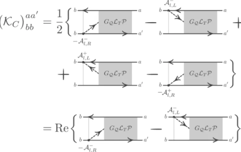
Figure 1.2.: Diagrammatic representation of the current Kernel for the current at lead l. First equality shows the sum over the four different contributions of the current Kernel in Eq. (1.45), corresponding to the left most vertex. The gray box stands for all possible irreducible diagrams contained in G_Q(0⁺)L_T. In the second equality we exploited the property that by moving all vertices to the opposite contour and reversing the arrows, two diagrams are complex conjugated.

1.2.1. Diagrammatic evaluation of the current Kernel

For a diagrammatic evaluation of the current Kernel, basically the same rules as for the master equation can be used, with the following exception. As we can see from Eq. (1.39) and Eq. (1.45), the left most vertex in the current Kernel stems from the current operator. Moreover, comparing Eq. (1.39) with Eq. (1.40), one notes that A⁻_l,L and A⁺_l,R have the opposite signs in the two equations. Therefore, we assign an additional minus sign to diagrams where the arrow associated to the left most vertex points away from the upper contour or towards the lower contour.

Fig. 1.2 depicts the exact current Kernel of lead l, where the diagrams come from the four different contributions of the current operator (Eq. (1.39)). The gray box in the diagrams represents all possible higher order irreducible contributions that can be constructed by contracting the left most vertex. Please note, that the complex conjugate of a diagram is obtained by moving all vertices to the opposite contour, and reversing the direction of the arrows on the fermion lines.[34, 36] Thus, two diagrams in Fig. 1.2 which are mapped into each other by moving the vertex to the opposite contour, and by reversing the direction of the fermion, are complex conjugated. This proves the last equality in Fig. 1.2. Importantly, the analysis in Fig. 1.2 shows that our definition of the current yields a real current to all orders in the coupling.

(29)

1.2. The current

Figure 1.3.: Diagrammatic representation of the second order current. As we have already seen in Fig. 1.2, contributions to the current Kernel are appearing in complex conjugated pairs, yielding the real part.

1.2.2. Second order approximation of the current

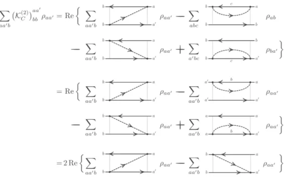
To fix the ideas we calculate the second order current explicitly. The lowest order approximation Eq. (1.44) reads as

Il(∞) = ∑

baa^′

TrB(⟪bb∣K˜⁽_C²⁾(0⁺)∣aa^′⟫⟪aa^′∣Pρˆ(∞)⟫), (1.46) where the trace over the system degrees of freedom is written in Liouville space, and we inserted an identity between the Kernel and the density matrix. Moreover, the second order current Kernel is given by

⟪bb∣K˜⁽²⁾

C (0⁺)∣aa^′⟫ = ∑

baa^′

⟪bb∣P I_l,LG˜₀(0⁺)L_TP ∣aa^′⟫. (1.47) In Fig. 1.3 we calculate the current, using only the diagrams. As we have seen already in Fig. 1.2, the diagrams appear always as sums of complex conjugated pairs and only their real part contributes to the current. In the first step of the diagrammatic calculation in Fig. 1.2 we renamed the summation variables, such that the density matrices have the same indices. Moreover, one sees from the

(30)

diagrammatic rules that, here, the diagrams with two vertices on one contour give the same, but negative analytical expression as the corresponding diagram with a diagonal fermion line. Hence, they are combined in the last equality of the calculation. Finally, the expression for the current can be read off easily. We find

I_l(∞) =e∑

baa^′

2 Re{ i

̵h∫

∞

−∞dE f⁺(E)G(E)g_NT⁻(a^′, b)T⁺(b, a) E+µ_l−E_ba+i0⁺ }ρ_aa^′

−e∑

baa^′

2 Re{i h̵ ∫

∞

−∞dE f⁻(E)G(E)gNT⁻(a^′, b)T⁺(b, a) E+µ_l−E_ab+i0⁺ }ρaa^′

(1.48)

Eq. (1.48) can be further simplified I_l(∞) =e∑

baa^′

((Γ^>_a′bba)

l− (Γ^<_a′bba)

l)ρaa^′, (1.49) where

(Γ^>_a′bba)

l=2π

̵h gNT⁻(a^′, b)T⁺(b, a)f⁺(E_ba−µ_l)G(E_ba−µ_l) (1.50) (Γ^<_a′bba)

l=2π

̵h g_NT⁻(a^′, b)T⁺(b, a)f⁻(E_ba−µ_l)G(E_ba−µ_l). (1.51) The rates are obtained from Eq. (1.48) by using the Dirac identity to solve the integral.

(31)

Superconducting Hybrid

Structures

(32)

(33)

Superconductor-quantum dot hybrid systems

The first part of the thesis addresses the transport properties of quantum dot structures coupled to one or two superconducting leads. The transport properties of these superconductor-quantum dot hybrid systems have been in the focus of research, both experimentally and theoretically, since their first experimental realizations in the 1990s.[45, 25, 26] As mentioned already in the introduction of the thesis, depending on the relation between the coupling strength Γ, the temperature T, the superconducting gap ∆, and the electron-electron interaction U, one differentiates various transport regimes. Here, we want to be more precise and give an overview of the different regimes and the expected transport behavior.

If Γ is the dominant energy scale, electron-electron interactions are negligible, and transport reduces to resonant tunnelling of quasi-particles and Cooper-pairs through the dot levels. In particular, coherent Cooper-pair tunnelling generates the supercurrent typical of the Josephson effect. [25]

In the weak coupling regime Γ≪U,∆, k_BT, on the other hand, transport is dominated by quasiparticle tunneling processes, as the tunneling of Cooper pairs is prevented by the dominant charging energyU ≫∆, k_BT. Here, a perturbation theory in the small parameter Γ can be developed. To lowest order O(Γ), it accounts for sequential tunneling events of quasiparticles, while cotunneling processes via virtual states of the quantum dot are incorporated in the next leading order O(Γ²). The main differences to the normal conducting case are caused by the sharply peaked energy dependent BCS-density of states, which suppresses quasiparticle states below the threshold energy ∆. Thus, beside the characteristic Coulomb diamond structure, an additional transport gap is observed for bias voltages ∣eV_b∣ < 2∆ in thedI/dVsd stability diagrams. First transport theories addressing this regime were presentede.g. in Ref. [46], using a master equation approach where the rates were calculated on the basis of Fermi’s golden-rule. As we will see in Chaps. 2 and 3, the superconductor quasiparticle density of states gives also rise to additional transport channels, opened by thermally excited quasiparticles for temperatures k_BT ≲∆, leading to additional subgap features.[46, 47, 48, 49]

In the intermediate coupling regime Γ is comparable to at least one of the other energy scales. This regime is the richest in different physical phenomena but also the most complicated to address theoretically and its full description is still a

(34)

junction behavior, and the multiple Andreev reflections and Andreev bound states.

[4, 5, 12, 6, 20, 10, 13, 8, 17, 50, 51, 42, 25, 26] In chapter 4 we focus instead on the intermediate coupling regime where Γ∼kBT, still keeping U ≫Γ and ∆≫Γ.

Similarly to the weak coupling regime, transport is here dominated by quasiparticle tunneling. However, renormalization effects caused by charge fluctuation processes become important. Specifically, the broadening of the transport features in the current is not only governed by the temperature, but also by the intrinsic level broadening. For normal conducting leads the intermediate coupling regime has been addressed already by various numerical methods,[52, 53] a second order von Neumann approach,[54, 55] the resonant tunneling approximation, [41, 34] and the dressed second order theory.[33, 56] The last two approaches are based on a master equation for the reduced density matrix, where the renormalization effects are caused by charge fluctuation processes. In the superconducting case, on the other hand, non-perturbative methods were used, for instance by Levy Yeyati et al. [50], who calculated the transport through a quantum dot in the limitU → ∞with a non equilibrium Green’s function approach. Governale et al.[42] applied the real time diagrammatic approach of Ref. [41, 34] to the case of superconducting leads and calculated non-perturbative contributions to the Josephson as well as the Andreev current in the limit ∆ → ∞ by resumming Cooper pair fluctuation diagrams to all orders.[51, 42] However, a theoretical investigation of the intermediate coupling regime (Γ∼k_BT) in the case of a quantum dot molecule with finite U coupled to superconducting leads of finite ∆ is still missing.

(35)

2. Subgap features due to thermally

excited quasiparticles in quantum dots coupled to superconducting leads

Parts of this chapter have been published in cooperation with Andrea Donarini, and Milena Grifoni in Ref. [47]

Based on the general discussion of the master equation in Chap. 1, we present here a microscopic theory for transport through superconductor-nanojunction hybrid systems in the sequential tunneling limit. In particular, we analyze the out- comes of the lowest order approximation of the Kernel, given in Eq. (1.29), in the case of superconducting leads in full details. With our method we differentiate from Ref. [46] by going beyond the constant interaction implicitly used there, and from Refs. [57] and [58] since we also treat subgap features associated to many- body excitations of a quantum dot molecule (double quantum dot). In contrast to Green’s function techniques, see e.g. Ref. [59], this method enables one to treat the interactions on the system exactly. Moreover, as shown on the example of a double quantum dot, our theory is easily scalable and allows an exact treatment of the Coulomb interaction and can treat any quantum dot set-up. Hence, we can describe lowest order quasiparticle transport of experimental relevant quantum dot systems (multiple quantum dots or multilevel quantum dots). We focus on transport involving thermally excited quasiparticles, and show that excited states of the quantum dot system can be observed in the current voltage spectroscopy in the Coulomb blockade region. Though transitions between two ground states are blocked due to the gap in the BCS-density of states, thermally excited quasiparticles can partici- pate in transport through excited system states, giving a source of subgap features in superconducting hybrid systems. These subgap features are already present in lowest order of the perturbation theory, in contrast to Cooper pair transport which occurs only in fourth order in the tunneling coupling. Nevertheless, experiments suggest the existence of a regime in which quasiparticle transport dominates also in the subgap region [25]. For a quantum dot coupled to a normal and a superconducting lead, a possible explanation for the subgap features observed in Ref.

(36)

[8] is given, where a carbon nanotube quantum dot is coupled to a normal and a superconducting contact.

This chapter is organized as follows: In Sect. 2.1 we introduce the Hamiltonian in a system-bath model using a number conserving version of the Bogoliubov-Valatin transformation [60, 61]. We describe the electrons of the superconducting leads as a combination of quasiparticle excitations of the BCS-ground state and Cooper pairs. For this purpose we introduce Cooper pair creation and annihilation operators. The explicit inclusion of these operators allows one to construct a theory which conserves the particle number in the tunneling process. In this way, for example, anomalous contributions to the tunneling rates due to Cooper pairing naturally vanish in second order. In Sect. 2.2, the generalized master equation for the reduced density matrix is derived and used to calculate the current. In Sect. 2.3 we apply the theory to the calculation of transport characteristics of two systems:

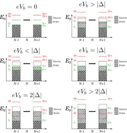
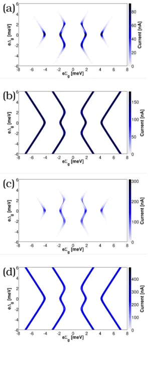
the single level quantum dot (SD) and the double quantum dot (DD), the latter in two possible configurations cf. Fig. 2.1. The SD is used to explain basic phenomena such as a gap opening in the Coulomb diamonds which is proportional to the superconducting gap, and transport involving thermally excited quasiparticles [46].

On the other hand, the DD possesses a richer many-body spectrum with several excited states. We visualize transitions through excited system states in the low bias regime using thermally excited quasiparticles. Due to the gap in the BCS- density of states, the ground state to ground state transition is not allowed in all cases, leading to transport through excited system states, appearing as peaks in the Coulomb blockade region. The threshold for observing excited system states in the subgap region is that the energy difference between the excited state and its ground state must be smaller than 2∣∆∣. We confirmed this threshold by means of the independently gated DD, where the detuning of the two sites changes the level spacing. Finally the N-QD-S system is investigated, where a quantum dot is coupled to a normal and a superconducting lead. In this case only the superconducting lead produces thermal lines in the Coulomb blockade region, giving a possible explanation for the subgap features in Ref. [8].

2.1. Model Hamiltonian

In the following chapter we consider quantum dot systems weakly coupled to two superconducting leads. The corresponding total Hamiltonian is written in a system- bath model:

Hˆ =HˆS+HˆB+HˆT, (2.1) where ˆHS represents the Hamiltonian of the quantum dot system, ˆHBis the Hamil- tonian of the superconducting leads, and ˆH_T describes the tunneling between the system and the leads. Specifically, we focus on two systems, a single level quantum