Edited by:
Alberto Basset, University of Salento, Italy
Reviewed by:
Daria Martynova, Zoological Institute (RAS), Russia Mario Barletta, Universidade Federal de Pernambuco (UFPE), Brazil
*Correspondence:
Sünnje L. Basedow sunnje.basedow@uit.no
Specialty section:
This article was submitted to Marine Ecosystem Ecology, a section of the journal Frontiers in Marine Science
Received:11 December 2017 Accepted:14 May 2018 Published:04 June 2018
Citation:
Basedow SL, Sundfjord A, von Appen W-J, Halvorsen E, Kwasniewski S and Reigstad M (2018) Seasonal Variation in Transport of Zooplankton Into the Arctic Basin Through the Atlantic Gateway, Fram Strait. Front. Mar. Sci. 5:194.
doi: 10.3389/fmars.2018.00194
Seasonal Variation in Transport of Zooplankton Into the Arctic Basin Through the Atlantic Gateway, Fram Strait
Sünnje L. Basedow1*, Arild Sundfjord2, Wilken-Jon von Appen3, Elisabeth Halvorsen1, Slawomir Kwasniewski4and Marit Reigstad1
1Arctic and Marine System Ecology, Faculty of Biosciences, Fisheries and Economy, UiT The Arctic University of Norway, Tromsø, Norway,2Norwegian Polar Institute, Tromsø, Norway,3Helmholtz Center for Polar and Marine Research, Alfred-Wegener-Institute, Bremerhaven, Germany,4Institute of Oceanology, Polish Academy of Sciences, Sopot, Poland
The largest contribution of oceanic heat to the Arctic Ocean is the warm Atlantic Water (AW) inflow through the deep Fram Strait. The AW current also carries Atlantic plankton into the Arctic Basin and this inflow of zooplankton biomass through the Atlantic-Arctic gateway far exceeds the inflow through the shallow Pacific-Arctic gateway. However, because this transport has not yet been adequately quantified based on observational data, the present contribution is poorly defined, and future changes in Arctic zooplankton communities are difficult to project and observe. Our objective was to quantify the inflow of zooplankton biomass through the Fram Strait during different seasons, including winter. We collected data with high spatial resolution covering hydrography (CTD), currents (ADCP and LADCP) and zooplankton distributions (LOPC and MultiNet) from surface to 1,000 m depth along two transects crossing the AW inflow during three cruises in January, May and August 2014. Long-term variations (1997–2016) in the AW inflow were analyzed based on moored current meters. Water transport across the inflow region was of the same order of magnitude during all months (January 2.2 Sv, May 1.9 Sv, August 1.7 Sv). We found a higher variability in zooplankton transport between the months (January 51 kg C s−1, May 34 kg C s−1, August 50 kg C s−1), related to seasonal changes in the vertical distribution of zooplankton. However, high abundances of carbon-rich copepods were observed in the AW inflow during all months. Surface patches with high abundances ofC. finmarchicus,Microcalanusspp.,Pseudocalanus spp., and Oithona similis clearly contributed to the advected biomass, also in winter.
The data reveal that the phenology of species is important for the amount of advected biomass, and that the advective input of zooplankton carbon into the Arctic Basin is important during all seasons. The advective zooplankton input might be especially important for mesopelagic planktivorous predators that were recently observed in the region, particularly during winter. The inflow ofC. finmarchicuswith AW was estimated to be in the order of 500,000 metric tons C y−1, which compares well to modeled estimates.
Keywords: advection, West Spitsbergen current, mesozooplankton, laser optical plankton counter, Atlantic Water, seasonal, Arctic Ocean, winter
INTRODUCTION
The Arctic marine environment has undergone major changes in temperature and ice cover over the last decades, and is projected to continue to warm and thaw (Overland and Wang, 2013; IPCC, 2014). The largest oceanic heat transport to the Arctic Basin is the warm Atlantic Water (AW) inflow through the deep Fram Strait (Beszczynska-Möller et al., 2011). Over the last decades this AW inflow has become warmer (Beszczynska-Möller et al., 2012), and it has been identified as the main mediator of climate change in the Arctic marine environment (Spielhagen et al., 2011; Polyakov et al., 2012; Onarheim et al., 2014). In addition to heat, the AW current transports phytoplankton (Hegseth and Sundfjord, 2008;
Metfies et al., 2016) and zooplankton of Atlantic origin, and with different functional roles (Kosobokova and Hirche, 2009; Kraft et al., 2013; Gluchowska et al., 2017b). Changes in ecosystem structure at lower latitudes are thus advected into the Arctic Basin and affect productivity and carbon cycling (Hunt et al., 2016).
The input of zooplankton biomass through the Atlantic-Arctic gateway far exceeds the input through the shallow Pacific-Arctic gateway due to the large differences in water volume advected (Bluhm et al., 2015; Wassmann et al., 2015). However, this input has not yet been adequately quantified based on observational data, therefore the present contribution is poorly defined, and future changes in Arctic Basin zooplankton communities are still difficult to project and observe.
Atlantic expatriates in the Arctic Basin can considerably influence the composition of Arctic zooplankton communities;
they might exert top-down control on primary production, and may also be an important food source for higher trophic levels (Olli et al., 2007; Kosobokova et al., 2011; Falk-Petersen et al., 2014). How the inflow of Atlantic species will manifest itself in Arctic food webs in the future is less clear. For example the Atlantic copepod Calanus finmarchicus contributes 30–40% to zooplankton biomass in the western Nansen basin (Mumm, 1993;
Kosobokova and Hirche, 2009; Wassmann et al., 2015), but so far this species has not been able to reproduce in the Arctic Ocean and high non-predatory mortality is observed (Hirche and Kosobokova, 2007; Daase et al., 2014). The reasons for this are not fully understood, but low temperatures in the upper layer may slow development considerably, leading to a failure of reaching the main overwintering stages within one season (Hirche and Kosobokova, 2007; Daase et al., 2014). The delayed onset of the phytoplankton bloom in the Arctic domain also impacts survival and reproductive success of Atlantic copepods, by hindering development, maturation and egg production the following spring (Niehoff and Hirche, 2000). A warmer AW current might thus not only bring new species into the Arctic Ocean, but may also affect survival of those that are transported there.
North Atlantic and Arctic zooplankton species have adapted their life cycles to the pronounced seasonality at higher latitudes.
Many herbivorours copepods tend to leave the productive epipelagic zone in winter, but variability occurs in the timing of their seasonal migrations throughout the Arctic (Daase et al., 2013). Other, omni- and detrivore species remain in the epipelagic (e.g., Oithona similis) or the mesopelagic zone (e.g.,
Triconia borealis) throughout the year, as a seasonal study from the Canadian Arctic has shown (Darnis and Fortier, 2014). The AW inflow in the Fram Strait stretches over the epipelagic into the mesopelagic zone and occupies roughly the upper 600–
800 m. Species that stay in the epipelagic throughout the year will thus be advected into the Arctic Basin continuously, while species that perform seasonal migrations below the AW will be advected mainly during spring and summer. Seasonal variability occurs also in the strength and extension of the AW inflow: in summer the baroclinic offshore branch of the West Spitsbergen Current (WSC) is absent (Wekerle et al., 2017), such that in winter the WSC tends to be wider and stronger with two-fold higher transport (Beszczynska-Möller et al., 2012). The interplay between the seasonality of the currents and the variable seasonal migrations of zooplankton as part of their life cycle therefore strongly affects the potential of different species to be advected into the Arctic Basin.
The dominating Atlantic copepodC. finmarchicushas its core habitat in the Norwegian Sea, where it migrates to depths below the AW layer for overwintering (Gaardsted et al., 2011). During spring and summer C. finmarchicus stays in the upper layer and is then advected with AW to areas downstream (Edvardsen et al., 2003). In the region of AW inflow into the Arctic Basin C. finmarchicusrecently has been observed in surface waters as early as January (Daase et al., 2014; Berge et al., 2015; Blachowiak- Samolyk et al., 2015). Winter data on zooplankton vertical distribution from Arctic regions are still scarce, but these recent observations challenge our understanding of the life cycle of one of the most well-studied copepods. A reduced understanding of fundamental principles also hinders the modeling of zooplankton transport into the Arctic Basin correctly, and stresses the need for seasonal observations.
Not all the AW that flows through the Atlantic gateway enters the Arctic Basin, in fact large amounts recirculate and eventually turn southwards (Hattermann et al., 2016; von Appen et al., 2016). However, a narrow barotropic branch flows northwards with high velocity along the steep continental slope in the eastern Fram Strait. Most of this water likely enters the Arctic Basin across the southeastern Yermak Plateau, although mesoscale instabilities shed off eddies that propagate westwards (Hattermann et al., 2016; von Appen et al., 2016). To the west of this continental slope current, to approximately 5◦E, the fate of the AW and included zooplankton is less certain. The AW flows northwards to the Yermak Plateau before either recirculating west- and southwards or entering the Arctic Basin across or around the perimeter of the plateau (Koenig et al., 2017). To the west of 5◦E the AW is likely recirculated. Zooplankton studies from the AW inflow in the northern Fram Strait so far have been limited to few (<10) stations and were mostly restricted to the upper 200 m (Hirche et al., 1991; Blachowiak-Samolyk et al., 2007; Svensen et al., 2011; Nöthig et al., 2015; Gluchowska et al., 2017a,b).
Time series of 9–14 years from the WSC indicate that with a warming AW we can expect higher abundances of the Atlantic- boreal speciesC. finmarchicus and Oithona similis(Weydman et al., 2014; Gluchowska et al., 2017a). However, based on optical data with high spatial resolution the generally patchy distribution
of zooplankton has been confirmed for a region of the AW inflow in the Fram Strait (Trudnowska et al., 2016). Spatial variability explained as much of the variability in the analyzed time series as environmental factors did (Weydman et al., 2014). Often, statistical analyzes of net samples are complicated by the spatial resolution of the nets not matching the spatial resolution of the physical parameters. In this respect optical and acoustical methods that are collected in concert with physical parameters have the potential to greatly enhance our understanding of factors governing zooplankton distributions (Wu et al., 2014). In addition, these methods allow the collection of high-resolution data both in the vertical and horizontal plane, which needs to be taken into account when quantifying advection of zooplankton into the Arctic Basin.
Our main objective is to quantify the zooplankton biomass entering the Arctic Basin through the Fram Strait during different seasons, including winter. Based on an extensive biophysical dataset with high spatio-temporal resolution we aim to answer (1) how the interplay between the seasonal variability in AW inflow and zooplankton vertical distributions determines the advection of zooplankton species with different life cycles, and (2) how the input of external zooplankton biomass into the Arctic Basin compares to Arctic secondary production.
MATERIALS AND METHODS Field Sampling
Physical-biological data on the seasonal variation in hydrography, currents and plankton distributions were collected with high spatial resolution along two transects (referred to as C and D for consistency with other publications in this issue) crossing the Atlantic Water inflow into the Arctic Basin during three research cruises with R/V Helmer Hanssen in January, May and August 2014 (Figure 1, Table 1). Only one transect was completed in January due to time constraints. During the research cruises, currents were measured using a ship-mounted Acoustic Doppler Current Profiler (ADCP, RDI 75 kHz) along transects and a lowered ADCP (LADCP, RDI 300 kHz) profiling at stations. For an increased temporal resolution we used data from 6 moorings placed in the study region in 2014, and analyzed variations in the northward flow of Atlantic Water in 2014 compared to the long-term mean from 1997 to 2016 (von Appen et al., 2016). The moorings were located along 78◦50′N, 79◦N and 79◦45′N near the 2,500 m isobaths. They contained rotor current meters and upward looking ADCPs at 250 m depth. More details on the mooring setup can be found in Beszczynska-Möller et al. (2012).
To obtain high spatial resolution data on water mass properties and plankton distributions we used a free-fall Moving Vessel Profiler (MVP, ODIM Brooke Ocean, Rolls Royce Canada Ltd., Herman et al., 1998) that was equipped with a Conductivity-Temperature-Depth and a Fluorescence sensor (CTD, Applied Microsystems Micro CTD; F, WET Labs FLRT Chlafluorometer), as well as a Laser Optical Plankton Counter (LOPC; ODIM-Brooke Ocean Rolls Royce Canada Ltd.,Herman et al., 2004). These instruments provide quantitative data at a rate of 4 Hz (CTD-F) or 2 Hz (LOPC) on hydrography,
fluorescence and mesozooplankton abundance. All instruments on the MVP are contained in a “fish” that is controlled by a remotely-operated winch system. In ice-free waters the MVP was used in free-wheel mode while the ship moved forward along transects. In this mode data are collected along profiles while the fish falls freely through the water column at 3.5–
4 m s−1 vertical speed, and is then retrieved automatically by the winch. Sampling depth was from surface to 10 m above the bottom, but restricted to 1,000 m at maximum, which is well below the Atlantic Water layer (Table 1). Ship velocity along transects was 6–7 knots (3–3.6 m s−1) and bottom depth ranged between ca. 200 m on the shelf to >1,000 m offshelf, resulting in a distance between starting points of individual profiles of ca. 0.5 km on the shelf and ca. 5.5 km offshelf. When ice conditions did not permit continuous sampling, single profiles were taken with the MVP and the winch was then operated in continuous rounds-per-minute mode, resulting in downward velocities of the fish of ca. 3 m s−1. Alternatively, if conditions in total were too risky to deploy the MVP (i.e., a combination of darkness, sea ice, strong winds and high waves), the LOPC was mounted on a sturdy rosette frame together with a different CTD (Seabird 19plusV2, Seabird Electronics Inc., USA) and fluorescence sensor (WETLabs EcoFl, Seabird Electronics Inc., USA). In this case the instruments were deployed vertically at stations along the transects, and lowered with a speed of 0.7–
0.8 m s−1.
To analyze the depth distribution of species and to aid interpretation of the high-resolution data, species composition in the study region was investigated based on vertically stratified net samples. These were collected by a MultiNet Midi (180µm mesh size, 0.25 m2mouth opening, Hydro-Bios, Kiel, Germany) that was deployed vertically at stations along transects (Table 1).
Hauling speed was 0.5 m s−1. Samples were preserved in a solution of 80% seawater and 20% fixation agent (75%
formaldehyde buffered with hexamine, 25% anti-bactericide propandiol), resulting in a final formaldehyde concentration of 4%.
Raw Data Analyses
Analyses of Water Masses
CTD data were screened for out-of-range values, which were removed prior to further analyses. Potential temperature (2) and density (σ2) were computed from a running mean over 2 m of pressure, temperature and salinity using the seawater package (version 3.3.4) in python (www.python.org, version 2.7). Based on this, T-S diagrams (not shown) were made to help identifying water masses.
Analyses of Water Currents
The climatological northward transport for each month of the year was established based on mean gridded current data from the moorings as described inBeszczynska-Möller et al. (2012), but the data set was extended by 2 years, ranging from 2002 to 2012. Not all the moorings could be recovered in 2015, therefore we followed the approach ofvon Appen et al. (2016) to judge how similar 2014 was compared to the climatology.
Current data obtained from the vessel-mounted ADCP and
FIGURE 1 |Map of the study area. The main inflow of Atlantic Water into the Arctic Basin is shown in red, afterHattermann et al. (2016). Continous sampling for hydrography and zooplankton distribution was performed along transects C and D (blue lines), which cross the Atlantic inflow. Magenta dots indicate mooring locations, pink stars indicate stations at which zooplankton was sampled.
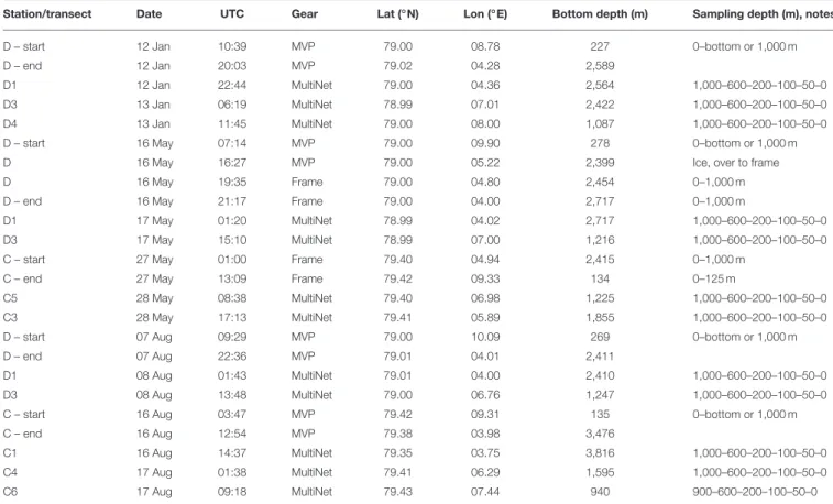
TABLE 1 |Seasonal sampling for mesozooplankton across the Atlantic Inflow west of Svalbard in January, May, and August 2014.
Station/transect Date UTC Gear Lat (◦N) Lon (◦E) Bottom depth (m) Sampling depth (m), notes
D – start 12 Jan 10:39 MVP 79.00 08.78 227 0–bottom or 1,000 m
D – end 12 Jan 20:03 MVP 79.02 04.28 2,589
D1 12 Jan 22:44 MultiNet 79.00 04.36 2,564 1,000–600–200–100–50–0
D3 13 Jan 06:19 MultiNet 78.99 07.01 2,422 1,000–600–200–100–50–0
D4 13 Jan 11:45 MultiNet 79.00 08.00 1,087 1,000–600–200–100–50–0
D – start 16 May 07:14 MVP 79.00 09.90 278 0–bottom or 1,000 m
D 16 May 16:27 MVP 79.00 05.22 2,399 Ice, over to frame
D 16 May 19:35 Frame 79.00 04.80 2,454 0–1,000 m
D – end 16 May 21:17 Frame 79.00 04.00 2,717 0–1,000 m
D1 17 May 01:20 MultiNet 78.99 04.02 2,717 1,000–600–200–100–50–0
D3 17 May 15:10 MultiNet 78.99 07.00 1,216 1,000–600–200–100–50–0
C – start 27 May 01:00 Frame 79.40 04.94 2,415 0–1,000 m
C – end 27 May 13:09 Frame 79.42 09.33 134 0–125 m
C5 28 May 08:38 MultiNet 79.40 06.98 1,225 1,000–600–200–100–50–0
C3 28 May 17:13 MultiNet 79.41 05.89 1,855 1,000–600–200–100–50–0
D – start 07 Aug 09:29 MVP 79.00 10.09 269 0–bottom or 1,000 m
D – end 07 Aug 22:36 MVP 79.01 04.01 2,411
D1 08 Aug 01:43 MultiNet 79.01 04.00 2,410 1,000–600–200–100–50–0
D3 08 Aug 13:48 MultiNet 79.00 06.76 1,247 1,000–600–200–100–50–0
C – start 16 Aug 03:47 MVP 79.42 09.31 135 0–bottom or 1,000 m
C – end 16 Aug 12:54 MVP 79.38 03.98 3,476
C1 16 Aug 14:37 MultiNet 79.35 03.75 3,816 1,000–600–200–100–50–0
C4 17 Aug 01:38 MultiNet 79.41 06.29 1,595 1,000–600–200–100–50–0
C6 17 Aug 09:18 MultiNet 79.43 07.44 940 900–600–200–100–50–0
The Moving Vessel Profiler (MVP) contained a laser optical plankton counter (LOPC) together with a CTD and a fluorescence sensor (F), continuous profiles were taken while moving along transects. Also the rosette frame (Frame) was equipped with a LOPC-CTD-F, it was deployed vertically at stations. The MultiNet was deployed vertically and sampled several depth layers. For details see section Materials and Methods.
L-ADCP data were first processed by standard routines and afterwards tides were subtracted based on AOTIM (Padman and Erofeeva, 2004). The current data along transects were
gridded using multivariate interpolation as specified in the function griddata in scipy.interpolate (www.scipy.org, version 0.18.1).
Two regions of possible inflow of AW into the Arctic Ocean were identified based on flux across transect D as observed by the moored instruments in this study, and as modeled in the study region (Hattermann et al., 2016): (1) The Inflow region in the upper 700 m along the continental slope between 8 and 9◦E, and (2) the Uncertain Fate region in the upper 700 m between 5.5 and 8◦E. Water and zooplankton in the Inflow region have a high likelihood of entering the Arctic Ocean, while in the Uncertain Fate region water and zooplankton may eventually end up in the Arctic Ocean or may be recirculated southwards in the East Greenland Current. We also analyzed the transport in the 700–
1,000 m layer below both regions to estimate the transport of zooplankton residing below the AW layer.
Analyses of Zooplankton Distributions
Zooplankton distributions were analyzed with high spatial resolution based on LOPC data. The LOPC counts and measures particles that pass through its sampling channel while the instrument is towed through the water (Herman et al., 2004).
Two types of particles are registered by the LOPC, single element particles (SEPs) and multi element particles (MEPs). SEPs are smaller particles which darken one to two of the 49 photodiodes of the LOPC, MEPs are larger particles that darken more than two photodiodes. Typically SEPs dominate in the size range below 0.6–0.8 mm equivalent spherical diameter (ESD), above which MEPs dominate. For MEPs additional features are registered, e.g., the transparency of particles, which is usually calculated as attenuation index (AI) that ranges from zero (completely transparent) to one (completely opaque). The size range of particles detected and registered by the LOPC is 0.1µm to 35 mm ESD, but only particles between ca. 0.2 and 4 mm ESD are counted quantitatively. We analyzed particles in this size range as described inBasedow et al. (2014), which included thoroughly checking the quality of the data as described in Schultes and Lopes (2009)and Espinasse et al. (2017). The ESD is a relative measure of the diameter a particle has, in case of the LOPC it is the diameter equivalent to black calibration spheres. This means for example that large, transparent particles can have a relatively small ESD. The LOPC does not give any taxonomic information, and nets are not suited to capture marine snow or fragile zooplankton. Therefore, it is often unclear if transparent particles are marine snow or transparent zooplankton, and this varies in all likelihood regionally and seasonally (Ohman et al., 2012; Basedow et al., 2013). To separate zooplankton from other particles we followed the method developed byEspinasse et al.
(2017)that indicates the ratio of zooplankton to detritus among small (SEPs) and large (MEPs) particles by analyzing two simple indicators, the percentage of MEPs in all counts, and the mean AI of MEPs.
During all months few faulty MEPs (as defined in Schultes and Lopes, 2009) were observed and the total number of MEPs was far below 106, showing that the LOPC was not overloaded and counted the correct amount of particles (Table A1). In January the mean AI was high (>0.2) and MEPs were relatively large (>1 mm ESD), which is typical for polar systems dominated by larger copepods (Basedow et al., 2013; Espinasse et al., 2017). In May and August parts of the transects (6 out
of 9 files) were characterized by a high percentage of MEPs (≥2%) in combination with a low (August) to very low AI (May), Table A1. This is typical for hydrologically stratified systems, when the LOPC counts phytoplankton aggregates, other detritus and/or transparent zooplankton along with more opaque zooplankton (Espinasse et al., 2017). In May very high chlorophyll concentrations (up to 11.6 mg m−3) were observed in the area, indicating that phytoplankton aggregates might have contributed to LOPC counts. In August chlorophyll concentrations were lower (<4 mg m−3) indicating that detritus and/or transparent zooplankton might have contributed most to the large amount of transparent particles. More information on the distribution of chlorophyll can be found inRandelhoff et al.
(this issue).
We divided particles into three different size groups and excluded transparent particles, i.e., MEPs with an AI < 0.4, from our analyses so that the large size group consisted of zooplankton only, while the medium size group consisted of zooplankton for the most part. For the small size group, which consists mostly of SEPs, a division based on the transparency of particles is not possible, therefore the small size group in May and August most likely consisted of a mixture of zooplankton and detrital material. In January, however, the indicators developed byEspinasse et al. (2017)and applied to our data suggest that the small size group consisted mostly of zooplankton. The following three size groups were analyzed:
small (S, 200–600µm ESD), medium (M, 0.6–1.5 mm ESD) and large particles (L, 1.5–4 mm ESD). This size classification was chosen to separate dominating species in the study area into different groups, where possible (Basedow et al., 2014, and references therein).
Abundance of the three size groups was estimated based on particle counts and the water volume flowing through the sampling channel. For data that were collected during retrieval of the MVP “fish,” the water volume calculated based on LOPC data differed strongly from the water volume estimated trigonometrically from wire length, cable speed and the ships velocity. It is uncertain which of the estimated volumes is the correct one, therefore we constrained abundance analyses to downward profiles.
Analyses of the Zooplankton Community
From the fixed MultiNet samples zooplankton were counted and identified to the level of species (most copepods), genus or family (other groups). Conspicuous, large zooplankton (>5 mm, chaetognaths >10 mm) were identified and enumerated from the entire sample. From the rest of the sample, at least 500 individuals from a minimum of three sub samples (2 ml, obtained with an automatic pipette with tip end cut to leave a 5 mm opening) were identified, staged to life cycle and counted. This procedure allows for the analysis of abundance of common species and taxa with 10% precision and at a 95%
confidence level (Postel, 2000). Copepods of the genusCalanus were identified to species based on their size (Kwasniewski et al., 2003). Specimens other than copepods were measured and sorted into different size categories (<5, 5–10, and 10–
20 mm).
Analyzing Seasonal Variation in Transport of Zooplankton Into the Arctic Ocean
Transport of zooplankton biomass (kg C s−1) across the four different areas (Inflow region, Uncertain Fate region, and the layers below both, see section Analyses of Water Currents) was calculated by multiplying mean biomass in an area (mg C m−3) with mean northward water transport across that area (in Sv = 106 m3 s−1). Mean northward water transport was calculated based on the long-term data from 1997 to 2012 (Beszczynska-Möller et al., 2012, 2015), because we judged this to be more representative for the seasonal variation than the short-term data from the ship-mounted ADCP. Due to eddy activity in the region measured currents at any given time are representative for a few days only. Biomass transport was calculated for January, May and August, which in combination with the vertical distribution of zooplankton allowed us to analyze seasonal variation in the advection of zooplankton. A two-factorial analysis of variances (ANOVA) was performed to test if the depth distribution of zooplankton was significantly different between months and transport regions. Mean biomass was determined based on the zooplankton biovolume observed by the LOPC in each area. For this, biovolume was converted into carbon using a fixed ratio of 0.03 mg C mm−3(Zhou et al., 2010).
Biomass data from the downward profiles were gridded using multivariate interpolation as specified in the function griddata in scipy.interpolate (www.scipy.org, version 0.18.1). For each area the average carbon content per m3 was then computed based on the gridded data. Incorrectly interpolated data from depths below sampled depths at the shelf break were excluded from the analyses.
RESULTS Water Masses
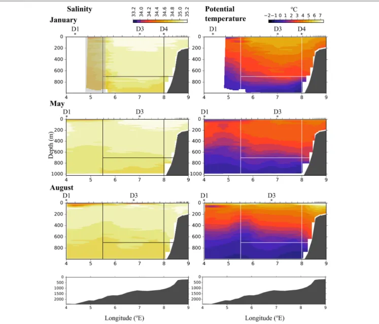
During all cruises the dominating water mass in the upper 500 m was Atlantic Water (AW,2 >2◦C,σT <27.97,Rudels et al., 2005),Figure 2. Along transect D in January AW was observed from surface down to ca. 700 m along most of the transect, and down to ca. 400 m west of 5.6◦E. West of 5.6◦E the conductivity sensor was not working properly and this area is indicated by a gray rectangle inFigure 2. Also in May and August AW was observed all along the transect, but stretched down to ca. 450 m only and was overlain by a layer (ca. 50 m) of warm Polar Surface Water (wPSW,2 >0◦C,σT<27.7,Rudels et al., 2005). The layer of wPSW originates from sea ice that is melted by the relatively warm AW or by solar radiation (Rudels et al., 2005), seeFigure 2 and Figure A1 for the distribution of wPSW along the transects in individual months. Below the warmer, less dense AW (2 >2◦C) a part of AW with lower temperature was observed, down to ca.
900 m in January and ca. 750 m in May and August. This colder, denser AW, often called Arctic Atlantic Water, is characterized by 0◦C< 2 <2◦C,σT>27.97,σ0,5<30.444, and by 2and salinity increasing with depth (Rudels et al., 2005; Marnela et al., 2016). The main water mass below both these AW water masses was characterized by2 <0◦C andσT>27.97, properties typical for Arctic Intermediate Water (AIW,Marnela et al., 2016).
Currents
Short-Term Currents Measured During the Cruises In the Inflow region along the shelf break between 8 and 9
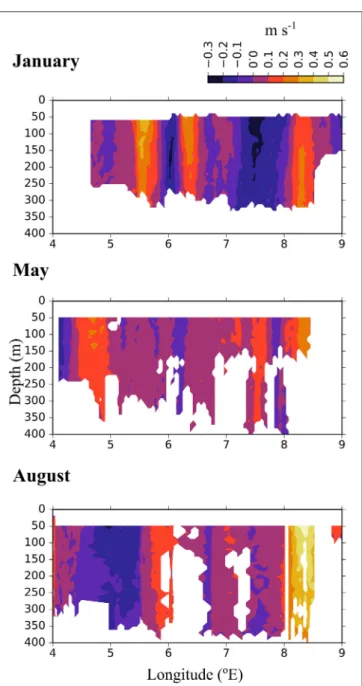
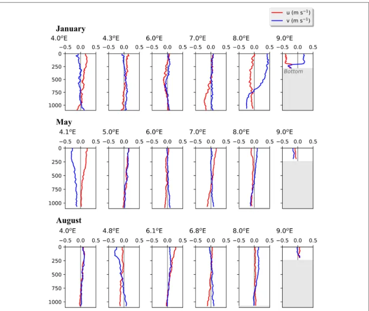
◦E, both the ship-mounted ADCP (Figure 3) and the lowered ADCP (Figure 4) recorded a northward directed flow during all months. According to the ship-mounted ADCP the northward current was fastest in August, with more than 50 cm s−1, in an area not sampled by the LADCP. Conversely, in January the LADCP measured high current speed with nearly 50 cm s−1at 8◦E, which was not detected by the ship-mounted ADCP. The northward flow was restricted to the upper 700 m during all sampled months. Below 700 m along the shelf break the current was flowing with variable velocities toward the southeast in January and May, and with low velocities toward the southwest in August (Figure 4). In the region of Uncertain Fate, between 5.5 and 8◦E, both instruments detected variable currents, with relatively strong northward velocities at times but also relatively strong southward velocities at other times, up to 30 cm s−1at ca.
7.5◦E in January (Figure 3, top). West of 8◦E current direction below 700 m was mostly toward the northwest and the current speed was mostly low (Figure 4).
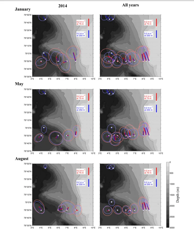
Long-Term Currents Observed by the Moorings The currents observed by the ship-mounted ADCP and the LADCP (Figures 3, 4) at transect D were generally consistent with the currents observed at the mooring locations (Figure 5).
Averaged over 1 to 31 January 2014 and 1 to 31 May 2014 a consistent northward flow at 75 m and 250 m was observed at the moorings along the continental slope (Figure 5). This is in agreement with the long-term measurements at the moorings, which showed a strong northward current in January, May and August (Figure 5, right panels). However, averaged over 1 to 31 August 2014 currents with highly variable directions were observed in the Inflow region, contrary to the long-term northward flow. During all months currents were more variable and weaker in the Uncertain Fate region than in the Inflow region along the shelf break. Currents at 250 m were not noticeably weaker than at 75 m (Figure 5), which is in agreement with the LADCP data that did not show a decrease in current velocity in the upper 500 m at most of the stations (Figure 4).
Zooplankton Distribution
The distribution of zooplankton in the area indicates their potential of entering the Arctic Basin, depending on their vertical position in the water column (upper part or at depths>600 m), and whether they are in the Inflow region (along the continental slope between 8 and 9◦E) or in the region of Uncertain Fate (5.5–8 ◦E). Significant seasonal differences were observed in the distribution of all zooplankton size groups (Figures 6–8, Table A2). In January, patches with high abundances of all size groups were observed in the surface layer, where they are subject to higher current velocities. Relatively high abundances were also observed below ca. 500 m, i.e., below the core of AW inflow (Table 2,Figures 6–8, top). In May, most medium- sized and large zooplankton was concentrated in AW, and very low abundances were observed below 700 m (Table 2, Figures 7,8). In August, medium and large zooplankton were
FIGURE 2 |Salinity(Left)and potential temperature(Right)along transect D in January(Top), May(Middle), and August(Bottom). Ticks along the top axis indicate start points for vertical sampling profiles. Stars with labels depict stations at which zooplankton was sampled. In January, the conductivity sensor was not working properly west of 5.6◦E, this area is indicated by a gray rectangle. Black(Left)and white(Right)lines indicate the areas that were used for calculating flux. The bottom panels show the bottom topography along the transect.
found in the entire water column, with the highest abundances of medium zooplankton in the upper 500 m (Figures 7, 8).
The surface patches in January consisted predominantly of Calanus finmarchicus CIV and CV, butMicrocalanusspp. and Pseudocalanus spp. also had high abundances, as well as the cyclopoid copepodOithona similis(Table 2, and data for specific depth layers, not shown). Below the AW water layer these species, along withMetridia longa, were by far the dominating constituents of the zooplankton community in January.
Relatively low abundances (<1,000 individuals m−3) of small plankton were observed offshelf between 100 and 200 m in January, and below 200 m east of 5 ◦E in May (Figure 6).
Significantly higher abundances were observed along the shelf
break in the Inflow region in January and also in May (Figure 6, Table A2). Keep in mind that the small size group likely contained a mixture of zooplankton and other particles in May and August, see Methods. In August, the distribution of small plankton and particles was very uniform along the transect, with very high abundances (between 104and 106m−3) in the epipelagic zone and high abundances (103-104 m−3) below (Figure 6). Net samples showed highest abundances of small zooplankton in the upper 600 m in May and August.
Very high abundances of copepod nauplii,Oithona similisand Microcalanus spp. were observed in May. In August copepod nauplii, young stages of C. finmarchicus, Microcalanus spp.
andOithona similisdominated.Triconia borealishad very high
FIGURE 3 |North-south directed current velocities across transect D, based on data collected by a ship-mounted ADCP during 3 months in 2014. The strong positive values east of 8◦E along the shelf break show the northward directed Atlantic inflow toward the Arctic Basin.
abundances below the AW layer in May, and in the AW layer in August.
The distribution of medium-sized zooplankton in January was similar to the distribution of small zooplankton in this month, with highest abundances in patches in the surface layer (up to 105 ind. m−3),Figure 7. Relatively high abundances (up to 1,000 ind. m−3) were also observed in the Inflow region along the shelf break, and in a large area below 400 m and between approximately 5.5 and 7.5 ◦E. The dominating species in the medium size group wereC. finmarchicusCII-CIV andMetridia longa(Table 2). In January and May, the areas of low abundances
of medium-sized zooplankton coincided with areas in which low abundances of small plankton and particles were observed. In August, the distribution of medium-sized zooplankton seemed to be less uniform than that of the small size group (Figure 7).
Lowest abundances were observed in the surface layer in the center of transect D, in wPSW, while highest abundances were observed in the center of transect C.
Large zooplankton was distributed more patchily than the other two size groups (Figure 8). C. finmarchicus CV was by far the dominating copepod in the large size group (Table 2, Figure 9) In January patches of more than 1,000 ind. m−3 were observed in the surface layer, and large zooplankton resided either close to the surface or below 600 m in the region of Uncertain Fate (Figure 8). In May, scattered patches were observed in AW along transect D, while highest abundances were found at the surface in wPSW along transect D and C. Almost all large zooplankton was concentrated in wPSW along transect C in May. The distribution of large zooplankton in August was patchy, but patches (with 100–1,000 ind. m−3) were distributed all along the transects and at all depths (Figure 8). Along transect C in August more patches were observed along the shelf break than farther west.
Zooplankton and Water Transport
Northward water transport across transect D was in the same order of magnitude during all months, but largest in January and lowest in August (Table 3). Across the Inflow region northward transport was roughly 2 Sv during all months, while transport across the Uncertain Fate region was more variable with approx.
3 Sv in January, 2 Sv in May, and 1 Sv in August. Below 700 m depth water transport was generally much lower with ca. 0.1 Sv below the Inflow region and 0.3–0.7 Sv below the Uncertain Fate region. These low transport rates nevertheless have the potential to transport substantial amounts of zooplankton residing at depth during the winter months.
Northward transport of zooplankton across the Inflow region during the different months was more variable than water transport (Table 3). In total about 50 kg C s−1were transported across the Inflow region in January and August, and are highly likely to reach the Arctic Basin and to impact the ecosystem there. In May the total amount of carbon transported was lower, with about 34 kg C s−1 (Table 3). Additionally, a large but variable amount of carbon was transported northward across the Uncertain Fate region.
About 9,000 individuals m−3of small zooplankton occurred in the Inflow region in January, mostly Microcalanus spp., Pseudocalanus spp., and Oithona similis (Table 2). This corresponded to a transport of ca. 11 kg C s−1 over the entire Inflow region (Table 3). In May and August about 19 kg C s−1of small plankton and particles were transported across the Inflow region. The relative contribution of non-zooplankton particles was likely highest at depth, below the Inflow and Uncertain Fate regions, where net samples showed relatively low abundances of small zooplankton, but where the LOPC recorded moderate to high numbers of plankton and particles (Table 2,Figure 6).
Across the Inflow region northward biomass transport of medium-sized zooplankton was lowest in May (ca. 4 kg C s−1),
FIGURE 4 |Vertical profiles of current velocities at six stations along transect D. Based on data collected by a lowered-ADCP during 3 months in 2014. Northward (v, blue) and eastward (u, red) directed currents are shown.
higher in August (ca. 14 kg C s−1) and highest in January (ca. 17 kg C s−1), Table 3. The medium size group consisted mostly of CII-CIV copepodids (Table 2), which in January and May were predominantly CIV, whereas in August they were CIII and CII (data not shown). The average carbon content per individual (mean biomass m−3divided by mean abundance m−3, Table 3) that was estimated for the medium group was lower in May than in January and August, and abundances were lower in May, resulting in a comparatively low biomass transport in May (Table 3). The high abundances of the dominating C. finmarchicus CIV in the upper layer in January (Table 2), together with the slightly higher average carbon content in this month (Table 3), and the slightly larger water transport compared to August, all resulted in the large transport of
medium-sized zooplankton carbon across the Inflow region in winter (Table 3).
The same tendency that was observed for the medium size group was also seen for the large size group. In January, large zooplankton resided in the upper layer, had a relatively high average carbon content and a relatively large water transport was measured. Thus, a high amount of large zooplankton biomass was transported across the Inflow region in January (23 kg C s−1, Table 3). Transport of large plankton across the Inflow region was also relatively high in May and August, 12 and 17 kg C s−1, respectively,Table 3. Substantial amounts of large zooplankton were also transported northward across the Uncertain Fate region, between 4 kg C s−1in May and 16 kg C s−1 in January (Table 3). Below the Inflow region transport differed by three
FIGURE 5 |Current strength and direction (lines) in an area of the Atlantic Water inflow toward the Arctic Basin during 3 months in 2014(Left), and averaged over 15 years from 1997 to 2012(Right). Based on moored ADCPs that were placed at 75 m (red) and 250 m (blue). The ellipses around the lines show standard deviations of the currents. The averaging period was January 1–31st (top), May 1–31st(Center), and August 1–31st(Bottom).
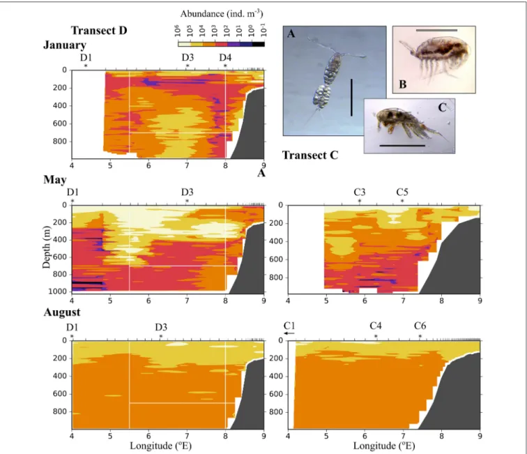
FIGURE 6 |Distribution of small plankton and particles (200–600µm equivalent spherical diameter) along three transects crossing the Atlantic inflow into the Arctic Basin. Based on data collected by a laser optical plankton counter (LOPC) in January(Top), May(Middle), and August(Bottom). SeeFigure 1for location of transects. Ticks along the top axis indicate start points for vertical sampling profiles with the LOPC, stars denote the approximate position of MultiNet stations that were sampled after completion of sampling with the LOPC. A small arrow indicates that the MultiNet station lay outside the transect. Three of the most abundant zooplankton species in the MultiNet samples in this size range are shown: (A)Oithona similis, (B)Microcalanussp., (C)Triconia borealis. The black scale bar is 0.5 mm, the gray scale bar is approximately 0.5 mm.
orders of magnitude between 2 g C s−1in January and 1 kg C s−1 in August.
DISCUSSION
This study provides the first quantification of abundance and biomass of zooplankton that flows with Atlantic Water (AW) through the Fram Strait into the Arctic Basin (AB). The occurrence of carbon-rich species in the upper 600 m, where northward current velocities were strongest, resulted in large
amounts of carbon being transported with the AW across the Inflow region. Furthermore, some of the zooplankton that is transported northward across the Uncertain Fate region may reach the AB, and likely more so in winter than in summer (Koenig et al., 2017). This suggest that the external input of zooplankton carbon, on the order of 34–50 kg C s−1 depending on the season (Table 3), is important for AW- influenced areas of the AB during all seasons, including winter.
Below we discuss how the interplay between zooplankton phenology and physical factors influences the advection of zooplankton into the AB (sections Zooplankton Phenology and
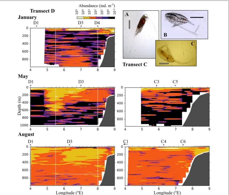
FIGURE 7 |AsFigure 6, but for medium-sized zooplankton (0.6–1.5 mm equivalent spherical diameter). (A)Heterorhabdus norvegicus(B)Calanus finmarchicusCIV, (C)Metridia longafemale. The black scale bar is 1 mm, the gray scale bar is approximately 1 mm.
Implications for Their Advection Toward the AB and Eddy Activity and Zooplankton Transport). Based on our data we perform calculations to relate our estimates of zooplankton input into the AB to observed and modeled zooplankton advection and to Arctic secondary production (sections Advection of the Atlantic Copepod C. finmarchicusto Implications of Advected Biomass for Arctic Productivity and Higher Trophic Levels).
Zooplankton Phenology and Implications for Their Advection Toward the AB
We observed a lower variability in water transport than in zooplankton transport between the months, indicating that zooplankton patchiness and vertical migrations influenced the advected biomass. Zooplankton patchiness is well known (e.g.,
Trudnowska et al., 2016) and also clearly visible in our data, e.g., when comparing the abundance of large zooplankton between transect D and C in May (Figure 8). This highlights the necessity to sample with high spatial resolution for an increased certainty when quantifying transport. Many species carried out seasonal vertical migrations between the upper 600 m and greater depths below the AW inflow (Table 2). In this study from an open ocean area with bottom depths >2,000 m we observed large and significant variations in vertical distribution of zooplankton between the months, also for those species that were mostly confined to certain depth ranges in the relatively shallow (<500 m) Amundsen Gulf of the Canadian Arctic (Darnis and Fortier, 2014). For example, the abundant, small cyclopoid Triconia borealisoccurred mostly below 600 m in January and
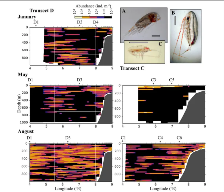
FIGURE 8 |AsFigure 6, but for large zooplankton (1.5–4 mm equivalent spherical diameter). (A)Paraeuchaetasp. (B)Calanus hyperboreus, (C)Calanus finmarchicusfemale. The gray scale bar is approximately 2 mm.
May, and mostly above 600 m in August. Thus, these copepods were transported rapidly northward in summer, when they stayed in the layer with higher current velocities, compared to winter and spring, when they stayed in the 700–1,000 m layer, where southward currents were observed and where northward transport was very small.
The occurrence of high abundances of C. finmarchicus CV in the upper layer in January contradicts their classic life cycle, which postulates that the copepods overwinter at depths below 600 m from late summer/autumn to early spring (e.g.,Edvardsen et al., 2006). Our observations are, however, in line with recent observations from the AW inflow region in January that also show high abundances of C. finmarchicus in the surface layer during winter months (Daase et al., 2014; Berge et al., 2015).
It is unclear how universal this observed behavior is, and if C. finmarchicusin this region does overwinter at depth at all, or if they stay in the upper layer throughout autumn and winter.
Our data indicate that the copepods might start their downward migration in August, when they were distributed over the entire water column, and might ascend already in December. In January high abundances were observed in the surface layer but also at greater depths. TheC. finmarchicusabundances observed in the surface layer in January were comparable to abundances observed elsewhere in its distribution range during summer (Melle et al., 2014).
This unexpected phenology has large impacts on the potential of these dominating copepods being advected into the AB.
Ontogenetic migrations may help to maintain populations at
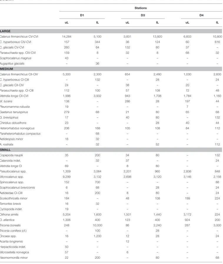
TABLE 2 |Abundance of zooplankton species (individuals m−2) collected by a 180µm-mesh MultiNet at stations across the Atlantic Water inflow into the Arctic Ocean in January, May and August 2014.
JANUARY
Stations
D1 D3 D4
uL lL uL lL uL lL
LARGE
Calanus finmarchicusCV-CVI 14,284 5,100 3,831 13,920 6,833 10,800
C. hyperboreusCIV-CVI 157 344 36 124 60 616
C. glacialisCV-CVI 260 64 132 80 37 –
Paraeuchaetaspp. CIV-CVI 159 8 32 8 68 32
Scaphocalanus magnus 43 – – – – –
Augaptilus glacialis – 36 – – – –
MEDIUM
Calanus finmarchicusCII-CIV 5,300 2,300 654 2,480 1,030 2,600
C. hyperboreusCI-CIII – 132 – 28 – 24
C. glacialisCII-CIV 24 – 38 – 20 –
Paraeuchaetaspp. CI-CIII 112 100 57 108 72 48
Metridia longaCII-CVI 1,996 3,932 943 1,708 1,784 1,160
M. lucens 138 – 286 28 197 44
Pleuromamma robusta 19 – – – 7 –
Gaetanus tenuispinus 279 68 21 80 65 68
G. brevispinus 17 – 40 80 – 132
Chiridius obtusifrons 23 – – 28 40 44
Heterorhabdus norvegicus 206 168 105 108 84 112
Paraheterorhabdus compactus – 68 – – – –
Aetideopsis minor 16 32 – – – –
A. rostrata – 32 – 52 – 112
SMALL
Copepoda nauplii 35 200 34 80 – 132
Calanoida indet. – 32 37 – – 24
Metridia longaCI 69 – 8 80 – –
Pseudocalanusspp. 1,309 3,064 2,201 960 2,836 848
Microcalanusspp. 9,299 3,132 2,698 3,120 3,146 2,156
Spinocalanusspp. 152 700 – – – 88
Scaphocalanus brevicornis 6 68 – 28 – 24
Aetideidae CI-CIII 16 200 8 80 – 24
Scolecithricella minor 184 – 48 108 199 224
Temorites brevis 16 32 – – – –
Cyclopoida indet. 19 – – – – –
Oithona similis 5,204 1,600 1,501 1,440 3,172 224
O. atlantica 1,306 400 123 400 924 200
Triconia borealis 248 10,000 86 2,240 287 3,000
Triconia conifera(cf.) – 100 – 28 – –
Oncaeaspp. 16 1,200 12 28 – 24
Acartia longiremis – – 12 – – –
Harpacticoida indet. 50 – – – – –
Microsetella norvegica 57 – 6 – – –
Neomormonilla minor 22 200 – 80 – 68
(Continued)
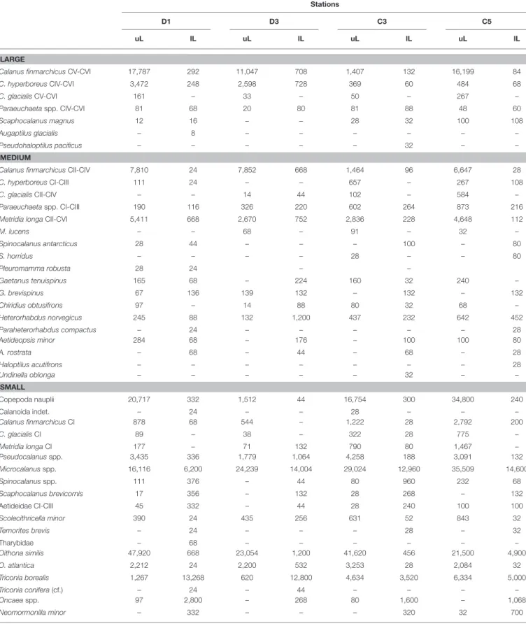
TABLE 2 |Continued MAY
Stations
D1 D3 C3 C5
uL lL uL lL uL lL uL lL
LARGE
Calanus finmarchicusCV-CVI 17,787 292 11,047 708 1,407 132 16,199 84
C. hyperboreusCIV-CVI 3,472 248 2,598 728 369 60 484 68
C. glacialisCV-CVI 161 – 33 – 50 – 267 –
Paraeuchaetaspp. CIV-CVI 81 68 20 80 81 88 48 60
Scaphocalanus magnus 12 16 – – 28 32 100 108
Augaptilus glacialis – 8 – – – – – –
Pseudohaloptilus pacificus – – – – – 32 – –
MEDIUM
Calanus finmarchicusCII-CIV 7,810 24 7,852 668 1,464 96 6,647 28
C. hyperboreusCI-CIII 111 24 – – 657 – 267 108
C. glacialisCII-CIV – – 14 44 102 – 584 –
Paraeuchaetaspp. CI-CIII 190 116 326 220 602 264 873 216
Metridia longaCII-CVI 5,411 668 2,670 752 2,836 228 4,648 112
M. lucens – – 68 – 91 – 32 –
Spinocalanus antarcticus 28 44 – – – 100 – 80
S. horridus – – – – 28 – – 80
Pleuromamma robusta 28 24 – –
Gaetanus tenuispinus 165 68 – 224 160 32 240 –
G. brevispinus 67 136 139 132 – 132 – 132
Chiridius obtusifrons 97 – 14 88 80 32 68 –
Heterorhabdus norvegicus 245 88 132 1,200 437 232 642 452
Paraheterorhabdus compactus – 24 – – – – – 28
Aetideopsis minor 284 68 – 176 – 100 100 80
A. rostrata – 68 – 44 – 68 – 28
Haloptilus acutifrons – – – – – – – 28
Undinella oblonga – – – – – 32 – –
SMALL
Copepoda nauplii 20,717 332 1,512 44 16,754 300 34,800 240
Calanoida indet. – 24 – – 28 – – –
Calanus finmarchicusCI 878 68 544 – 1,222 28 2,792 200
C. glacialisCI 89 – 38 – 322 28 775 –
Metridia longaCI 177 – 71 132 790 80 1,467 –
Pseudocalanusspp. 3,435 336 1,779 1,064 4,258 188 3,091 132
Microcalanusspp. 16,116 6,200 24,239 14,004 29,024 12,960 35,509 14,600
Spinocalanusspp. 111 376 – 44 80 960 232 68
Scaphocalanus brevicornis 17 356 – 132 28 268 – 132
Aetideidae CI-CIII 45 332 – 44 28 240 100 100
Scolecithricella minor 390 24 435 256 631 52 843 32
Temorites brevis – 24 – – – 28 – 32
Tharybidae – 68 – – – – – –
Oithona similis 47,920 668 23,054 1,200 41,620 456 21,500 4,900
O. atlantica 2,212 24 2,200 532 3,253 28 2,084 32
Triconia borealis 1,267 13,268 620 12,800 4,634 3,520 6,334 5,000
Triconia conifera(cf.) – 24 – 44 – – – –
Oncaeaspp. 97 2,800 – 268 80 1,600 – 1,068
Neomormonilla minor – 332 – – – 320 32 700
(Continued)