Tests of Power Corrections for Event Shapes in e

arXiv:hep-ex/0105059v2 23 Jul 2001

MPI-Ph/2001-005 Revised version, February 27, 2019

Tests of Power Corrections for Event Shapes

in e ⁺ e ⁻ Annihilation

P.A. Movilla Fern´ andez, S. Bethke, O. Biebel, S. Kluth

Max-Planck-Institut f¨ ur Physik, Werner-Heisenberg-Institut

F¨ohringer Ring 6 80805 Munich, Germany

Abstract

A study of perturbative QCD calculations combined with power corrections to model hadronisation effects is presented. The QCD predictions are fitted to differential distributions and mean values of event shape observables measured in e

e

annihi- lation at centre-of-mass energies from √ s = 14 to 189 GeV. We investigate the event shape observables thrust, heavy jet mass, C-parameter, total and wide jet broad- ening and differential 2-jet rate and observe a good description of the data by the QCD predictions. The strong coupling constant α

( M

) and the free parameter of the power correction calculations α

(2 GeV) are measured to be

α

( M

Z⁰

) = 0 . 1171

and α

(2 GeV) = 0 . 513

.

The predicted universality of α

is confirmed within the uncertainties of the mea- surements.

Acc. by Eur. Phys. J. C

1 Introduction

The study of hadronic final states in e

e

annihilation allows precise tests of the theory of strong interaction, Quantum Chromo Dynamics (QCD), using event shape observables for the analysis of hadronic events. For event shape observables perturbative QCD predictions in O (α

) and in some cases also in the next-to-leading-logarithm-approximation (NLLA) are available. The various experiments at the PETRA, PEP, TRISTAN, LEP and SLC colliders collected a large amount of data at centre-of-mass (cms) energies √ s = 14 to 189 GeV which can be used to make precise quantitative tests of QCD.

Precision tests of perturbative QCD from hadronic event shapes require a solid un- derstanding of the transition from the perturbatively accessible partons to the observed hadrons, the hadronisation process. Hadronisation effects cannot be described directly by perturbative QCD and are usually estimated by phenomenological hadronisation models available from Monte Carlo event generators, e.g. JETSET/PYTHIA [1], HERWIG [2]

or ARIADNE [3].

Alternatively, analytical approaches are pursued in order to deduce as much infor- mation as possible about hadronisation from the perturbative theory. Hadronisation contributions to event shape observables evolve like reciprocal powers of the hard inter- action scale √

s (power corrections) [4, 5]. An analytic model by Dokshitzer, Marchesini and Webber (DMW) of hadronisation valid for some event shape observables derives the structure of the power corrections from perturbative QCD. The model assumes that the strong coupling remains finite at low energy scales where simple perturbative calculations break down [6, 7]. The model parametrises the magnitude of non-perturbative effects by introducing moments of the running strong coupling α

as parameters to be determined by experiment.

Several experimental tests of power corrections in the DMW model with differential distributions or 1st moments (mean values) of event shape observables measured in e

e

annihilation have been done [7–16]. In the present paper we test power corrections in the DMW model to the differential distributions and mean values of event shape observables measured in e

e

annihilation experiments at √ s = 14 to 189 GeV.

We use resummed O (α

)+NLLA QCD calculations combined with power corrections to fit the event shape distributions with α

(M

) and the non-perturbative parameter α

as free parameters. In the case of the mean values O (α

) calculations together with power corrections are fitted to the data. We investigate the prediction of the DMW model that the non-perturbative parameter does not depend on the specific event shape observable, i.e. that it is universal.

Section 2 starts with an overview of the observables and briefly explains the theoretical predictions. The data used in our study and the fit results are presented in section 3. In section 4 we give a summary and draw conclusions from our results.

2 QCD Predictions

2.1 Event Shape Observables

We employ the differential distributions and mean values of the event shape observables thrust, heavy jet mass, C-parameter, total and wide jet broadening. The mean value of the differential 2-jet rate based on the Durham algorithm is used as well. The definitions of these observables are given in the following:

Thrust T The thrust value is given by the expression [17, 18]

T = max

~ n

P

i

| ~p

· ~n |

P

i

| ~p

|

!

.

where ~p

are the momentum vectors of the particles in an event. The thrust axis ~n

is the vector ~n which maximises the expression in parentheses. We use 1 − T in this analysis, because in this from the distribution is comparable to those of the other observables. A plane perpendicular to ~n

through the origin divides the event into two hemispheres H

and H

which are used in the defintion of heavy jet mass and the jet broadening observables below.

Heavy Jet Mass M

The invariant mass M

of all particles contained in hemisphere H

or H

is calculated [19]. The observable M

is defined by

M

= max(M

, M

)/ √ s .

Some experiments use the definition M

= max(M

, M

)

/s where in O (α

) we have the relation 1 − T = M

.

Jet Broadening The jet broadening measures are calculated by [20]:

B

=

P

i∈Hk

| ~p

× ~n

| 2 ^P

| ~p

|

for each hemisphere H

, k = 1, 2. The total jet broadening is given B

= B

+ B

and the wide jet broadening is defined by B

= max(B

, B

).

C-parameter The C-parameter is defined as [21, 22]

C = 3(λ

λ

+ λ

λ

+ λ

λ

)

where λ

, k = 1, 2, 3, are the eigenvalues of the momentum tensor Θ

=

P

i

(p

p

)/ | ~p

|

P

i

| ~p

| , α, β = 1, 2, 3 .

Differential 2-jet rate The differential 2-jet rate is determined using the Durham jet

finding algorithm [23]. In this algorithm the quantity y

= 2 min(E

, E

)(1 −

cos θ

)/E

, E

= ^P

E

, is computed for all pairs of (pseudo-) particles with

energies E

, E

in the event. The pair with the smallest y

is combined into a

pseudo particle by adding the 4-vectors and the procedure is repeated until all

y

> y

. The value of y

where the number of jets in an event changes from

three to two is called y

. The differential 2-jet rate is defined by the differential

distribution of y

.

2.2 Perturbative QCD predictions

We use QCD predictions in O (α

) matched with resummed NLLA calculations in our analysis of differential distributions [24–26]. In the NLLA the cumulative distribution R(y) = ^R

1/σ

(dσ/dy

)dy

of an observable y is considered. The NLLA is valid in re- gions of phase space where y is small, i.e. where the emission of multiple soft gluons from a system of approximately back-to-back and hard quarks dominates (2-jet region).

QCD predictions in O (α

) are expected to be valid in regions of phase space where em- mission of a single hard gluon dominates (3-jet region). We choose to combine the O (α

) with the NLLA calculations with the ln(R)-matching scheme, because it has theoretical advantages [7, 24] and is also preferred in experimental analysis [8, 27–33]. Other match- ing schemes exist and will be considered in the study of systematic uncertainties, see section 3.4 below.

The complete perturbative QCD prediction renormalised at the scale µ

for a cumula- tive distribution R

(y) using the ln(R)-matching scheme takes the following form [24,27]:

ln R

(y) = Lg

(L α ˆ

(µ

)) + g

(L α ˆ

(µ

)) (1)

− (G

L + G

L

) ˆ α

(µ

) − (G

L

+ G

L

) ˆ α

(µ

) +A(y) ˆ α

(µ

) +

B(y) − 2A(y) − 1 2 A(y)

ˆ

α

(µ

) ,

where L = ln(1/y ) and ˆ α

= α

/(2π). The functions g

and g

represent the all-orders resummations of leading and subleading logarithmic terms, respectively, and the G

coefficients are given e.g. in [27]. The coefficient functions A(y) and B(y) are defined by A(y) = ^R

(dA/dy

)dy

and B(y) = ^R

(dB/dy

)dy

, respectively. The differential distribu- tions dA/dy and dB/dy are obtained by integration of the O (α

) QCD matrix elements using the program EVENT2 [34]. The prediction is normalised to the total hadronic cross section evaluated in O (α

).

The renormalisation scale µ

is identified with the cms energy √

s = Q of the measure- ment. The dependence of the perturbative QCD predictions on the renormalisation scale is studied by introducing the renormalisation scale parameter x

= µ

/Q and making the replacements of [27], equation (23).

The mean values of event shape observable distributions are defined by h y i =

Z

0

y 1

σ

dσ

dy dy , (2)

where y

is the largest possible value of the observable y (kinematic limit). The per- turbative QCD prediction of mean values h y i

in O (α

) is given by

h y i

= A

α ˆ

(µ

) + B

+ (πβ

ln(x

) − 1)2 A

α ˆ

(µ

) (3)

where β

= (33 − 2n

)/(12π) with the number of active quark flavours n

= 5 at the

cms energies considered here. The O (α

) and O (α

) coefficients A

and B

are taken

from [35]. Calculations of mean values in NLLA are not yet available, because the NLLA predictions diverge for very small values of y and do not vanish at the kinematic limits y

of the observables.

2.3 Power Corrections

Non-perturbative effects to event shape observables are calculated in the DMW model as contributions from gluon radiation at low energy scales where perturbative evolution of the strong coupling breaks down. The location of the divergence in the perturbative evolution of α

, known as the Landau pole, is given by Λ

≃ 200 MeV in the MS renormalisation scheme. The model assumes that the physical strong coupling remains finite at scales around and below the Landau pole. A new free non-perturbative parameter

α

(µ

) = 1 µ

Z

0

α

(k)dk (4)

is introduced to parametrise the unknown behaviour of α

(Q) below the so-called infrared matching scale µ

. The non-perturbative and the perturbative evolution of the strong coupling are merged at the scale µ

which is generally taken to be 2 GeV [36].

The power corrections are calculated including two loop corrections for the differential distributions of the event shape observables considered here [13, 36]. The effect of hadro- nisation on the distribution obtained from experimental data is described by a shift of the perturbative prediction away from the 2-jet region:

dσ

dy = dσ

dy (y − P D

) , (5)

where y = 1 − T , M

, C, B

and B

. The factor P depends on non-perturbative parameter α

and is predicted to be universal [36]:

P = 4C

π

M µ

Q α

(µ

) − α

(µ

) − β

α

(µ

)

2π ln µ

µ

+ K β

+ 1

!!

(6) with the colour factor C

= 4/3. The factor K = (67/18 − π

/6)C

− (5/9)n

originates from the choice of the MS renormalisation scheme. The Milan factor M accounts for two-loop effects and its numerical value is 1.49 [37]. The theoretical uncertainty of M is about 20% due to missing higher order corrections [36]. The quantity D

depends on the observable [13, 36]:

D

= 2 , D

= 1 , D

= 3π , (7) D

= a

ln 1

b + F

(b, α

(bQ)) , b = B

, B

, a

= 1, a

= 1 2 .

A simple shift is expected for 1 − T , M

and C whereas for the jet broadening variables B

and B

an additional squeeze

of the distribution is predicted. The more complex

1

The term “squeeze” refers to the form of event shape distributions which are more peaked in pertur-

bative predictions compared to the predictions including hadronisation effects.

behaviour for the jet broadening observables calculated in [13] is related to the inter- dependence of non-perturbative and perturbative effects which cannot be neglected for these observables. The power corrections for B

and B

predict in addition to the shift an increasing squeeze with decreasing cms energies. The necessity of an additional non- perturbative squeeze of the jet broadening distributions was already pointed out in [15].

The power corrections for mean values of 1 − T , M

and C are obtained by taking the first moment of equation (5) and read:

h y i = h y i

+ P D

. (8) In the case of mean values of B

and B

the predictions from [13] are used. For the ob- servable y

the leading power correction is expected to be of the type 1/Q

or (ln Q)/Q

[6]

but the corresponding coefficients are not yet calculated.

3 Analysis of the Data

3.1 Data Sets

Experimental data below the Z

peak are provided by the experiments of the PETRA (12 to 47 GeV, about 50000 events in total), PEP (29 GeV, about 28000 events in total) and TRISTAN (55 to 58 GeV, about 1200 events in total) colliders. Data around the Z

resonance are from the four LEP experiments with O (10

) events per experiment and from SLD (about 40000 events) while data above the Z

are exclusively from the LEP experiments with O (10

) events per experiment from √

s = 133 to 183 GeV and O (10

) per experiment at √

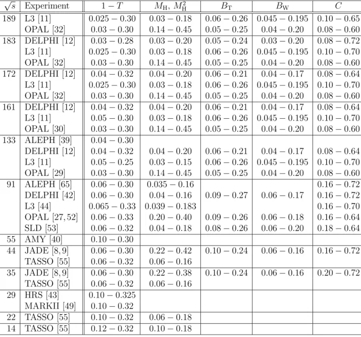
s = 189 GeV. For event shape distributions table 1 gives the references and also the ranges considered in the fits (see section 3.2 below). For mean values we consider published data available in the energy range of 13 up to 189 GeV [8, 10–12, 29, 30, 32, 38–55]. All data used in this study are corrected for the limited resolution and acceptance of the detectors and event selection criteria and are published with statistical and experimental systematic uncertainties.

3.2 Fit Procedure

The standard analyses use the entire data sets as described above. For the perturbative predictions of differential distributions we employ the matched resummed O (α

)+NLLA QCD prediction given by equation (1) while the power corrections are implemented accord- ing to equation (5). For mean values the O (α

) perturbative prediction from equation (3) is used combined with the power corrections according to equation (8).

For each observable we perform simultaneous χ

-fits with α

(M

) and α

(2 GeV) as free parameters. The strong coupling α

(M

) is evolved to the renormalisation scale µ

= x

Q with Q = √

s of a given event shape distribution or mean value using the two-

loop formula for the running coupling [56]. The χ

is defined by χ

= ^P

((d

− t

)/σ

)

where d

is the value of measurement i, t

is the corresponding theoretical prediction and

σ

is the quadratic sum of statistical and experimental systematic uncertainties of d

.

The fit ranges for fits of event shape distibutions are defined individually for each cms energy such that the 2-jet region of the distribution is exploited as far as possible.

The fit ranges are limited by the demands i) that the χ

of the extreme bins do not contribute substantially to the total χ

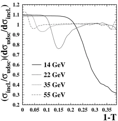
of the distribution, ii) that the perturbative QCD prediction is reliable, and iii) that the power corrections are under control. Requirement iii) is checked by monitoring the ratio of the theoretical predictions without and with power corrections, respectively, using the fit results for α

(M

) and α

(2 GeV). Figure 1 (solid lines) presents these ratios for 1 − T , M

, M

, B

, B

and C at √

s = 35 GeV. The fit ranges are chosen such that regions of rapidly varying power corrections are excluded.

The chosen fit ranges are listed in table 1.

3.3 Effects of bb Events at low √ s

The presence of events from the reaction e

e

→ bb at low cms energies √ s can distort the event shape distributions, because the effects of weak decays of heavy B-hadrons on the topology of hadronic events cannot anymore be neglected. An additional problem arises from comparing QCD calculations based on massless quarks with data containing massive quarks at √

s close to the production threshold.

At √

s ≪ M

bb events constitute about 9% of the total event samples. Ideally one would correct the data experimentally by identifying bb events and removing them from the sample. However, since we have only published event shape data without information on specific quark flavours we resort to a correction based on Monte Carlo simulations.

We generate samples of 10

events at each √

s with the JETSET 7.4 program [1] with the parameter set given in [57]. For each event shape observable we build the ratio of distributions calculated with u, d, s and c quark events to those calculated with all events. This ratio is multiplied with the bin contents of the data to obtain corrected distributions. This procedure is applied to all data at √ s < M

. We correct the mean values for the contribution from b quarks using exactly the same procedure as for the correction of the differential distributions. It was verified that the simulation provides an adequate description of the data at all values of √ s < M

. Figure 2 shows the ratio of distributions of 1 − T calculated using u, d, s, and c quark events or all events obtained at √

s = 14 to 55 GeV as an example. The correction is reasonable within the fit ranges at √

s > 14 GeV while at √

s = 14 GeV the correction is a large effect.

Systematic effects due to uncertainties in the Monte Carlo parameters are expected to be small for the ratio except for those parameters which only affect the bb events in the samples. The most important such parameter is the value of ε

in the Peterson fragmentation function [58] which controls the fragmentation of b quarks in the simulation.

Threshold effects on the fraction of bb events at low √

s which depend on the value of the

b-quark mass in the simulation are found to be negligible for the fit results.

3.4 Fit and Systematic Uncertainties

We consider the following for both fits to differential distributions and to mean values unless specified otherwise:

Fit error The fit errors for α

(M

) and α

(2 GeV) are taken from the diagonal elements of the error matrix after the fit has converged.

Renormalisation scale Systematic uncertainties from perturbation theory are assessed by varying x

between 0.5 and 2.0. The changes in the fit results w.r.t. the standard results are taken as asymmetric systematic uncertainties. In the case that both deviations have the same sign the larger one defines a symmetric uncertainty.

Matching scheme As a further systematic check in the analysis of differential dis- tributions we use different matching schemes, namely the modified ln(R)- and R-matching schemes, to combine the O (α

) with the resummed NLLA calcula- tions [27]. A possible matching scheme uncertainty is defined by the larger deviation caused by using ln(R)- or R-matching.

Power corrections Uncertainties due to the power corrections come from the choice of the value of µ

and from the theoretical uncertainty of the Milan factor M . We vary µ

by ± 1 GeV and M by ± 20% and take in both cases changes of the fit results w.r.t. the standard results as asymmetric systematic uncertainties. No error contribution from the variation of µ

is assigned to α

(µ

), because setting µ

to a different value corresponds to a redefinition of α

(µ

).

Fragmentation of b quarks The standard analysis is carried out with corrected data at

√ s < M

based on the JETSET tuning of [57] as explained in section 3.3. The value of the JETSET parameter ε

is varied around its central value ε

= 0.0038 ± 0.0010 by adding or subtracting its error and the analysis including correction of the data at √

s < M

is repeated. Deviations w.r.t. the standard results are considered as asymmetric uncertainties.

Experimental uncertainties We examine the dependence of the results on the input data taken for the fits in several ways:

1. We perform the fit without the LEP/SLC data at √

s ≃ M

.

2. In the case of fits to distributions the fits are repeated using seperately either the data below or above the Z

peak. This also checks for possible higher order non-perturbative contributions to the power corrections. Such tests are impractical with mean values, because the sensitivity to the power corrections is reduced when only restricted ranges in √

s are used, in particular for √

s > M

.

3. A further source of systematic uncertainty in the analysis of differential distri-

butions only comes from the choice of the fit ranges. The lower and the upper

edges of the fit ranges of all distributions of a given observable are varied in

both directions by one bin. We take the largest of the four deviations w.r.t.

the standard result as a systematic uncertainty.

For distributions the largest deviation from 1. and 2. w.r.t. the standard results is added in quadrature with the uncertainty from 3. and the result defines a symmetric systematic uncertainty. For mean values only the deviation from 1. is taken to define a symmetric systematic uncertainty.

The total errors of the standard results are defined as the quadratic sum of the fit errors, the renormalisation scale uncertainty, the power correction and the experimental uncertainties. In the case of distributions the larger of the matching scheme and the renor- malisation scale uncertainties is included in the total error and the fit range uncertainty is added as well.

3.5 Results of Fits to Event Shape Distributions

Our standard results for an observable are obtained with x

= 1 and µ

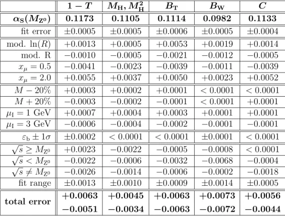
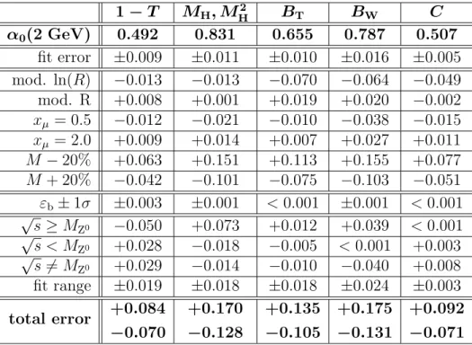
= 2 GeV. The results from the fits are listed in tables 2 and 3 for α

(M

) and α

, respectively. The signed values indicate the direction in which α

(M

) and α

(2 GeV) changed w.r.t. the standard analysis when systematic effects are studied. The fit curves of the standard results and the corresponding experimental data for 1 − T , M

or M

, C, B

and B

are shown in figures 3 to 6. Values of χ

/d.o.f . and of the correlation coefficients from the fits are given in table 4.

We generally observe a good agreement of the predictions with the data within the fit ranges, as indicated by the values of χ

/d.o.f .The two fit parameters are anticorrelated with a correlation coefficient ρ

≃ − 80%. The results for α

(M

) and α

(2 GeV) are consistent with each other within the total errors in the case of 1 − T , C and B

.

The agreement between data for B

at √

s < M

and the QCD prediction is not as good as with the other observables, see also table 4. The value for α

(M

) obtained for B

is about 15% smaller than the values from the other observables. In the case of B

the QCD prediction in the 3-jet regions tends to lie above the data leading to smaller values of α

(M

) in the fit. Fitting only data at √

s < M

leads to a significant deviation of α

(M

) w.r.t. the standard result, see table 2. This may indicate that √

s-dependent non-perturbative effects are not fully modelled by the calculations for B

.

In order to disentangle the different contributions to this effect we performed a fit of

the O (α

) QCD prediction for B

combined with power corrections with α

(M

), x

and

α

(2 GeV) as free parameters and obtained α

(M

) = 0.106 ± 0.001, x

= 0.10 ± 0.02

and α

(2 GeV) = 0.65 ± 0.03 with χ

/d.o.f . = 0.5. Since the value for α

(M

) is

comparatively small and the value for α

(2 GeV) is comparatively large we conclude that

both the O (α

)+NLLA perturbative predictions and the power correction calculations

contribute to the small values of α

(M

) and large values of α

(2 GeV) observed in

the standard fits. Small values of α

(M

) in fits with B

using O (α

)+NLLA QCD

calculations have also been observed in [8, 9, 27, 53, 59–61].

The results for α

(2 GeV) are consistent with each other within about two standard deviations of the total errors; in particular the values for α

(2 GeV) from M

or M

and B

are approximately 25% larger than the other results. We note the coincidence that M

and B

are calculated using only the hemispheres containing more invariant mass or transverse momentum, respectively. We conclude that α

(2 GeV) is approxiately universal within the total uncertainties of the individual measurements. The results for α

(2 GeV) are also consistent with earlier measurements [9, 11, 12].

The values of α

(M

) obtained from the fits are systematically lower than correspond- ing results which use the same O (α

)+NLLA perturbative predictions but apply Monte Carlo corrections instead of power corrections [8, 9, 27, 53, 59–61]. From the experimental point of view there is a lucid explanation for the differences between the α

(M

) results based on the power corrections and those based on Monte Carlo corrections [15]. The lat- ter induce a stronger squeeze to all distributions than the power corrections which simply predict a shift for 1 − T , M

and C without any presence of a squeeze. Although the situation improved for the jet broadening observables due to the revised calculations [13]

the effect of the squeeze remains below the expectation of the Monte Carlo hadronisation models. As a consequence the two-parameter fit favours smaller values for α

(M

) in order to make the predicted shape more peaked in the 2-jet region and hence chooses large values for α

in order to compensate the shift of the distribution towards the 2-jet region.

Figure 1 compares hadronisation corrections as predicted by power corrections and by the JETSET Monte Carlo program as used in section 3.3. The hadronisation corrections from the Monte Carlo simulation are defined as the ratio of distributions calculated using the partons left at the end of the parton shower (parton-level) and the stable particles (τ > 300 ps) after hadronisation and decays (hadron-level). In all cases and in particular for M

and B

the Monte Carlo corrections increase the slopes of the perturbative predictions more than the power corrections leading to larger values of α

(M

) in fits of the predictions to the data.

It turns out that the power correction uncertainties for α

(M

) are negligible for each observable while there are significant power correction uncertainties for α

. We conclude that α

(M

) is mainly constrained by the perturbative prediction rather than by the power correction contributions while α

is mostly determined by the power correction calculations. The strong dependence of α

on M is due to the anticorrelation seen in equation (6).

The total errors are generally dominated by the theoretical uncertainties. We observe significant variations of α

(M

) from B

and B

when considering only data with √

s <

M

in the fits; for B

this variation is the largest contribution to the total error of

α

(M

). For the jet broadening observables the matching scheme uncertainty is larger

than the renormalisation scale uncertainty for α

(2 GeV) and also for α

(M

) in the

case of B

. We also notice that the α

(2 GeV) results from B

and M

or M

have the

largest power correction uncertainties.

3.6 Results of Fits to Mean Values

The main fits to the mean values of 1 − T , M

, B

, B

and C are performed with α

(M

) and α

(2 GeV) as free parameters using x

= 1 and µ

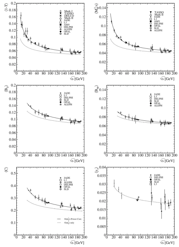
= 2 GeV. In figure 7 the results of the fits and the corresponding perturbative contribution h y i

of equation (8) are shown. The size of the power suppressed contribution is the difference between the dashed and the solid curves in figure 7. Tables 5 and 6 list the results of the fits and the variations found from the studies of systematic uncertainties.

We find that the fitted QCD predictions describe the data well with χ

/d.o.f. ≃ 1.

The fit results for α

(M

) and α

(2 GeV) for all observables are consistent with each other within their total errors and have correlation coefficients ρ

≃ − 90%. The results are also generally consistent with the results from fits to distributions. We note that in contrast to the analysis of distributions the results for α

(M

) and α

(2 GeV) from M

and B

are compatible with results from the other observables.

For the observable h y

i we investigated power corrections of the form 1/Q

, (ln Q)/Q

, 1/Q, (ln Q)/Q and omitting power correction terms, introducing α

(µ

) = (1/µ

)

· ^R

k · α

(k)dk as the second and an unknown coefficient D

as the third fit parameter [35, 62].

All fits yielded χ

/d.o.f. ≃ 1. For the 1/Q and (ln Q)/Q corrections large values for α

(M

) were obtained which are incompatible with the world average [63] within the fit errors. Corrections of the 1/Q

and (ln Q)/Q

type gave 1 to 2% increased values of α

(M

) and a value of α

(2GeV) = 0.25 ± 0.03(fit). The results for D

were − 0.2 and

− 0.4 for 1/Q

and (ln Q)/Q

, respectively, but also consistent with zero within the fit errors. We conclude that the data prefer one of these latter types of power corrections although the size of the correction is too small to be determined from the available data.

The smallness of the fitted D

coefficient justifies to neglect any power correction for fits of the h y

i data and we only quote the result of such fits in table 5. The result for α

(M

) from h y

i is also in good agreement with the world average value of the strong coupling.

3.7 Combination of Individual Results

The individual results are combined to single values for α

(M

) and α

(2 GeV), respec- tively, following the procedure described in [8, 27]. The combination is done separately for the results from event shape distributions or mean values. A weighted average of the individual results is calculated with the square of the reciprocal total errors used as the weights. For each of the systematic checks the weighted averages for α

(M

) and α

(2 GeV) are also determined and the total error of the weighted average is calcu- lated exactly as described in section 3.4. This procedure accounts for correlations of the systematic errors.

We obtain as combined results from the analysis of distributions

α

(M

) = 0.1111 ± 0.0004(fit) ± 0.0020(syst.)

(theo.)

α

(2 GeV) = 0.579 ± 0.005(fit) ± 0.011(syst.)

(theo.) .

The error contributions refer to the fit error (fit), the variations of the input data sets and the fit ranges (syst.) and the variations of the matching scheme, renormalisation scale, Milan factor and ε

(theo.). The total correlation coefficient is estimated as ρ = − 0.16 (see below). The small value for α

(M

) compared to the world average α

(M

) = 0.1181 ± 0.0034 [63] is caused by the small values of α

(M

) from M

or M

and in particular B

. If the results from B

are omitted from the weighted averages the results become α

(M

) = 0.1126

and α

(2 GeV) = 0.558

. This value for α

(M

) is in better agreement with the world average and with other measurements [9,27,53,59–61]

while the result for α

(2 GeV) changes only slightly.

The results from the study of mean values based on h 1 − T i , h M

i , h B

i , h B

i and h C i are

α

(M

) = 0.1187 ± 0.0014(fit) ± 0.0001(syst.)

(theo.) α

(2 GeV) = 0.485 ± 0.013(fit) ± 0.001(syst.)

(theo.) .

The error contributions are defined as explained above for distributions. The estimate of the total correlation coefficient is ρ = +0.17. The values for α

(M

) and α

(2 GeV) are in reasonable agreement with the results from distributions, especially when the average of results from distributions is calculated without the values from B

.

Figures 8 a) and b) present the results for α

(M

) and α

(2 GeV) with error ellipses based on the total errors. The correlation coefficients are determined as follows. For ev- ery systematic test a covariance matrix is constructed using the systematic uncertainties, symmetrised if neccessary, and a correlation coefficient ρ

. In cases where the correla- tion between systematic deviations of α

(M

) and α

(2 GeV) of a given systematic test has the same sign as the correlation ρ

from the fit result we set ρ

= ρ

. In cases where the signs from the correlations from the standard fit and the systematic test are opposite we set ρ

= +1 or − 1 taking the sign from the correlation of the systematic test. All covariance matrices are added and the result defines the error ellipsis. Tables 4 and 5 show the correlation coefficients obtained with this procedure. The correlation coef- ficients of the averages are calculated as the weighted averages of the individual correlation cofficients using the products of the individual total errors for α

(M

) and α

(2 GeV) as weights. The figure illustrates that the individual results for α

(M

) and α

(2 GeV) from distributions and mean values are compatible with each other and with the averages within the total errors. We consider this as a confirmation of the predicted universality of the non-perturbative parameter α

.

Finally we combine the results for α

(M

) from the analysis of distributions, mean values of 1 − T , M

, B

, B

and C and from h y

i by calculating error weighted averages based on the symmetrised total errors. As errors of the final combined results the smaller of the errors of the individual results are chosen. The final result for α

(M

) is

α

(M

) = 0.1171

.

The final result for α

(2 GeV) is obtained by combining the results from distributions

and mean values again quoting the smaller of the total errors of the individual results as

the final errors:

α

(2 GeV) = 0.513

.

The total correlation coefficient is again estimated as a weighted average of the correlation coefficients from the combined results from distributions and mean values, respectively, yielding ρ = +0.07.

4 Summary and Conclusions

The analytic treatment of non-perturbative effects to event shape observables in e

e

annihilation based on power corrections was examined. We tested predictions for the differential distributions and mean values of the observables 1 − T , M

or M

, B

, B

, C and y

, respectively. For this test a large amount of event shape data collected by several experiments over a range of e

e

annihilation energies from √

s = 14 to 189 GeV was considered.

Fits of perturbative QCD predictions combined with power corrections to distribu- tions and mean values of event shape observables were performed with the strong coupling α

(M

) and the non-perturbative parameter α

(µ

) as free parameters. The good quality of the fits with χ

/d.o.f . ≃ 1 supports the predicted 1/Q evolution of the power correc- tions. The results for α

(M

) and α

(2 GeV) from distributions are more consistent with each other compared to previous studies [15,16] due to the improved predictions of power corrections to the jet broadening variables. However, we still observe a large deviation of the α

(M

) results obtained from B

from those extracted from the other observables.

We conjecture that this discrepancy is a combined effect of the perturbative O (α

)+NLLA predictions and the power correction calculations for this observable. The individual re- sults for α

(M

) from all observables are observed to be systematically smaller than the corresponding results in [9, 27, 53, 59–61], which use Monte Carlo hadronisation models.

This observation may be related to the different amounts of squeeze of the distributions predicted by both types of hadronisation model.

We obtain as combined results for the strong coupling constant and the non-perturbative parameter:

α

(M

) = 0.1171

α

(2 GeV) = 0.513

.

It should be noted that the values for α

(M

) and α

(2 GeV) from B

are only compat- ible with the combined result and with the values of α

(M

) from the other observables within about two standard deviations of the total errors.

The average value for α

(2 GeV) is in good agreement with previous results [9, 35, 64].

The scatter of α

(2 GeV) values derived from 1 − T , B

and C is covered by the expected theoretical uncertainty of the Milan factor of about 20% [36].

Since this value is representative of the individual results within the errors we consider

this as a confirmation of the universality of α

as predicted by the DMW model. However,

the results from M

or M

and B

from distributions indicate that uncalculated higher orders may contribute significantly to the non-perturbative corrections.

References

[1] T. Sj¨ostrand: Comput. Phys. Commun. 82 (1994) 74

[2] G. Marchesini et al.: Comput. Phys. Commun. 67 (1992) 465 [3] L. L¨onnblad: Comput. Phys. Commun. 71 (1992) 15

[4] B.R. Webber: Phys. Lett. B 339 (1994) 148

[5] Yu.L. Dokshitzer, B.R. Webber: Phys. Lett. B 352 (1995) 451

[6] Yu.L. Dokshitzer, G. Marchesini, B.R. Webber: Nucl. Phys. B 469 (1996) 93 [7] Yu.L. Dokshitzer, B.R. Webber: Phys. Lett. B 404 (1997) 321

[8] P.A. Movilla Fern´andez, O. Biebel, S. Bethke, S. Kluth, P. Pfeifenschneider and the JADE Coll.: Eur. Phys. J. C 1 (1998) 461

[9] O. Biebel, P.A. Movilla Fern´andez, S. Bethke and the JADE Coll.: Phys. Lett. B 459 (1999) 326

[10] DELPHI Coll., P. Abreu et al.: Z. Phys. C 73 (1997) 229 [11] L3 Coll., M. Acciarri et al.: Phys. Lett. B 489 (2000) 65 [12] DELPHI Coll., P. Abreu et al.: Phys. Lett. B 456 (1999) 322

[13] Yu.L. Dokshitzer, G. Marchesini, G.P. Salam: Eur. Phys. J. direct C 3 (1999) 1 [14] O. Biebel: Nucl. Phys. Proc. Suppl. 64 (1998) 22

[15] P.A. Movilla Fern´andez: Nucl. Phys. Proc. Suppl. 74 (1999) 384 [16] D. Wicke: Nucl. Phys. Proc. Suppl. 64 (1998) 27

[17] S. Brandt, Ch. Peyrou, R. Sosnowski, A. Wroblewski: Phys. Lett. 12 (1964) 57 [18] E. Fahri: Phys. Rev. Lett. 39 (1977) 1587

[19] T. Chandramohan, L. Clavelli: Nucl. Phys. B 184 (1981) 365

[20] S. Catani, G. Turnock, B.R. Webber: Phys. Lett. B 295 (1992) 269

[21] G. Parisi: Phys. Lett. B 74 (1978) 65

[22] J.F. Donoghue, F.E. Low, S.Y. Pi: Phys. Rev. D 20 (1979) 2759 [23] S. Catani et al.: Phys. Lett. B 269 (1991) 432

[24] S. Catani, L. Trentadue, G. Turnock, B.R. Webber: Nucl. Phys. B 407 (1993) 3 [25] Yu.L. Dokshitzer, A. Lucenti, G. Marchesini, G.P. Salam: J. High Energy Phys. 1

(1998) 011

[26] S. Catani, B.R. Webber: Phys. Lett. B 427 (1998) 377 [27] OPAL Coll., P.D. Acton et al.: Z. Phys. C 59 (1993) 1 [28] OPAL Coll., R. Akers et al.: Z. Phys. C 68 (1995) 519 [29] OPAL Coll., G. Alexander et al.: Z. Phys. C 72 (1996) 191 [30] OPAL Coll., K. Ackerstaff et al.: Z. Phys. C 75 (1997) 193

[31] JADE and OPAL Coll., P. Pfeifenschneider et al.: Eur. Phys. J. C 17 (2000) 19 [32] OPAL Coll., G. Abbiendi et al.: Eur. Phys. J. C 16 (2000) 185

[33] S. Kluth, P.A. Movilla Fern´andez, S. Bethke, C. Pahl P. Pfeifenschneider: MPI- PhE/2000-19, hep-ex/0012044 (2000), Sub. to Eur. Phys. J. C

[34] S. Catani, M.H. Seymour: Phys. Lett. B 378 (1996) 287 [35] O. Biebel: Phys. Rep. 340 (2001) 165

[36] Yu.L. Dokshitzer, A. Lucenti, G. Marchesini, G.P. Salam: J. High Energy Phys. 5 (1998) 003

[37] Yu.L. Dokshitzer: hep-ph/9911299 (1999), Invited talk at 11th Rencontres de Blois:

Frontiers of Matter, Chateau de Blois, France, 28 Jun - 3 Jul 1999 [38] ALEPH Coll., D. Buskulic et al.: Z. Phys. C 55 (1992) 209

[39] ALEPH Coll., D. Busculic et al.: Z. Phys. C 73 (1997) 409

[40] AMY Coll., Y.K. Li et al.: Phys. Rev. D 41 (1990) 2675

[41] DELCO Coll., M. Sakuda et al.: Phys. Lett. B 152 (1985) 399

[42] DELPHI Coll., P. Abreu et al.: Z. Phys. C 73 (1996) 11

[43] HRS Coll., D. Bender et al.: Phys. Rev. D 31 (1985) 1

[44] L3 Coll., B. Adeva et al.: Z. Phys. C 55 (1992) 39

[45] M. Acciarri et al.: Phys. Lett. B 411 (1997) 339

[46] L3 Coll., M. Acciarri et al.: Phys. Lett. B 371 (1996) 137 [47] L3 Coll., M. Acciarri et al.: Phys. Lett. B 404 (1997) 390 [48] L3 Coll., M. Acciarri et al.: Phys. Lett. B 444 (1998) 569 [49] MARK II Coll., A. Petersen et al.: Phys. Rev. D 37 (1988) 1 [50] MARK J Coll., D.P. Barber et al.: Phys. Rev. Lett. 43 (1979) 901 [51] MARK J Coll., D.P. Barber et al.: Phys. Lett. B 85 (1979) 463 [52] OPAL Coll., P.D. Acton et al.: Z. Phys. C 55 (1992) 1

[53] SLD Coll., K. Abe et al.: Phys. Rev. D 51 (1995) 962

[54] TASSO Coll., W. Braunschweig et al.: Z. Phys. C 41 (1988) 359 [55] TASSO Coll., W. Braunschweig et al.: Z. Phys. C 47 (1990) 187

[56] R.K. Ellis, W.J. Stirling, B.R. Webber: QCD and Collider Physics. Vol. 8 of Cam- bridge Monographs on Particle Physics, Nuclear Physics and Cosmology, Cambridge University Press (1996)

[57] OPAL Coll., G. Alexander et al.: Z. Phys. C 69 (1996) 543

[58] C. Peterson, D. Schlatter, I. Schmitt, P. Zerwas: Phys. Rev. D 27 (1983) 105 [59] DELPHI Coll., P. Abreu et al.: Z. Phys. C 59 (1993) 21

[60] ALEPH Coll., D. Decamp et al.: Phys. Lett. B 284 (1992) 163 [61] L3 Coll., O. Adriani et al.: Phys. Lett. B 284 (1992) 471

[62] P.A. Movilla Fern´andez, O. Biebel, S. Bethke: PITHA 99/21, hep-ex/9906033 (1999) [63] S. Bethke: J. Phys. G 26 (2000) R27

[64] S. Kluth: MPI-PhE/2000-20, hep-ex/0009066 (2000)

[65] ALEPH Coll., R. Barate et al.: Phys. Rep. 294 (1998) 1

Tables

√ s Experiment 1 − T M

, M

B

B

C

189 L3 [11] 0.025 − 0.30 0.03 − 0.18 0.06 − 0.26 0.045 − 0.195 0.10 − 0.65 OPAL [32] 0.03 − 0.30 0.14 − 0.45 0.05 − 0.25 0.04 − 0.20 0.08 − 0.60 183 DELPHI [12] 0.03 − 0.28 0.03 − 0.20 0.05 − 0.24 0.03 − 0.20 0.08 − 0.72 L3 [11] 0.025 − 0.30 0.03 − 0.18 0.06 − 0.26 0.045 − 0.195 0.10 − 0.70 OPAL [32] 0.03 − 0.30 0.14 − 0.45 0.05 − 0.25 0.04 − 0.20 0.08 − 0.60 172 DELPHI [12] 0.04 − 0.32 0.04 − 0.20 0.06 − 0.21 0.04 − 0.17 0.08 − 0.64 L3 [11] 0.025 − 0.30 0.03 − 0.18 0.06 − 0.26 0.045 − 0.195 0.10 − 0.70 OPAL [32] 0.03 − 0.30 0.14 − 0.45 0.05 − 0.25 0.04 − 0.20 0.08 − 0.60 161 DELPHI [12] 0.04 − 0.32 0.04 − 0.20 0.06 − 0.21 0.04 − 0.17 0.08 − 0.64 L3 [11] 0.05 − 0.30 0.03 − 0.18 0.06 − 0.26 0.045 − 0.195 0.10 − 0.70 OPAL [30] 0.03 − 0.30 0.14 − 0.45 0.05 − 0.25 0.04 − 0.20 0.08 − 0.60 133 ALEPH [39] 0.04 − 0.30

DELPHI [12] 0.04 − 0.32 0.04 − 0.20 0.06 − 0.21 0.04 − 0.17 0.08 − 0.64 L3 [11] 0.05 − 0.25 0.03 − 0.15 0.06 − 0.26 0.045 − 0.195 0.10 − 0.70 OPAL [29] 0.03 − 0.30 0.14 − 0.45 0.05 − 0.25 0.04 − 0.20 0.08 − 0.60

91 ALEPH [65] 0.06 − 0.30 0.035 − 0.16 0.16 − 0.72

DELPHI [42] 0.06 − 0.30 0.04 − 0.16 0.09 − 0.27 0.06 − 0.17 0.16 − 0.72

L3 [44] 0.065 − 0.33 0.039 − 0.183 0.16 − 0.70

OPAL [27, 52] 0.06 − 0.33 0.20 − 0.40 0.09 − 0.26 0.06 − 0.18 0.16 − 0.64 SLD [53] 0.06 − 0.32 0.04 − 0.18 0.08 − 0.26 0.06 − 0.20 0.18 − 0.64 55 AMY [40] 0.10 − 0.30

44 JADE [8, 9] 0.06 − 0.30 0.22 − 0.42 0.10 − 0.24 0.06 − 0.16 0.16 − 0.72 TASSO [55] 0.06 − 0.32 0.06 − 0.16

35 JADE [8, 9] 0.06 − 0.30 0.22 − 0.38 0.10 − 0.24 0.06 − 0.16 0.20 − 0.72 TASSO [55] 0.06 − 0.32 0.06 − 0.16

29 HRS [43] 0.10 − 0.325 MARKII [49] 0.10 − 0.32

22 TASSO [55] 0.10 − 0.32 0.06 − 0.18 14 TASSO [55] 0.12 − 0.32 0.10 − 0.18

Table 1: The sources of the data and the fit ranges for the observables 1 − T , M

or M

,

B

, B

and C are shown. The cms energy √ s at which the experiments analysed their

data is given in GeV. The observable M

is used only by OPAL and JADE while M

is

used by the other experiments.

1 − T M

, M

B

B

C α

(M

) 0.1173 0.1105 0.1114 0.0982 0.1133

fit error ± 0.0005 ± 0.0005 ± 0.0006 ± 0.0005 ± 0.0004 mod. ln(R) +0.0013 +0.0005 +0.0053 +0.0019 +0.0014 mod. R − 0.0010 − 0.0005 − 0.0021 − 0.0012 − 0.0005 x

= 0.5 − 0.0041 − 0.0023 − 0.0039 − 0.0011 − 0.0039 x

= 2.0 +0.0055 +0.0037 +0.0050 +0.0023 +0.0052 M − 20% +0.0003 +0.0002 +0.0001 < 0.0001 < 0.0001 M + 20% − 0.0003 − 0.0002 − 0.0001 < 0.0001 +0.0001 µ

= 1 GeV +0.0007 +0.0004 +0.0003 +0.0001 +0.0001 µ

= 3 GeV − 0.0006 − 0.0004 − 0.0002 − 0.0001 − 0.0001 ε

± 1σ ± 0.0002 < 0.0001 < 0.0001 ± 0.0001 < 0.0001

√ s ≥ M

+0.0023 − 0.0022 − 0.0005 − 0.0008 < 0.0001

√ s < M

− 0.0022 − 0.0006 − 0.0032 − 0.0068 − 0.0004

√ s 6 = M

− 0.0026 − 0.0014 − 0.0006 − 0.0002 − 0.0018 fit range ± 0.0013 ± 0.0010 ± 0.0009 ± 0.0014 ± 0.0005 total error +0 . 0063 +0 . 0045 +0 . 0063 +0 . 0073 +0 . 0056

− 0.0051 − 0.0034 − 0.0063 − 0.0072 − 0.0044

Table 2: Values of α

(M

) are shown derived from fits of resummed O (α

)+NLLA

QCD predictions combined with power corrections to distributions of the event shape

observables 1 − T , M

or M

, B

, B

and C. In addition, the statistical and systematic

uncertainties are given. Signed values indicate the direction in which α

(M

) changed

with respect to the standard analysis.

1 − T M

, M

B

B

C α

(2 GeV) 0.492 0.831 0.655 0.787 0.507

fit error ± 0.009 ± 0.011 ± 0.010 ± 0.016 ± 0.005 mod. ln(R) − 0.013 − 0.013 − 0.070 − 0.064 − 0.049 mod. R +0.008 +0.001 +0.019 +0.020 − 0.002 x

= 0.5 − 0.012 − 0.021 − 0.010 − 0.038 − 0.015 x

= 2.0 +0.009 +0.014 +0.007 +0.027 +0.011 M − 20% +0.063 +0.151 +0.113 +0.155 +0.077 M + 20% − 0.042 − 0.101 − 0.075 − 0.103 − 0.051 ε

± 1σ ± 0.003 ± 0.001 < 0.001 ± 0.001 < 0.001

√ s ≥ M

− 0.050 +0.073 +0.012 +0.039 < 0.001

√ s < M

+0.028 − 0.018 − 0.005 < 0.001 +0.003

√ s 6 = M

+0.029 − 0.014 − 0.010 − 0.040 +0.008 fit range ± 0.019 ± 0.018 ± 0.018 ± 0.024 ± 0.003 total error +0.084 +0.170 +0.135 +0.175 +0.092

− 0.070 − 0.128 − 0.105 − 0.131 − 0.071

Table 3: Values of α

are shown derived from fits of resummed O (α

)+NLLA QCD pre- dictions combined with power corrections to distributions of the event shape observables 1 − T , M

or M

, B

, B

and C. In addition, the statistical and systematic uncertainties are given. Signed values indicate the direction in which α

changed with respect to the standard analysis.

1 − T M

, M

B

B

C

standard fit 172/263 137/161 91.9/159 96.1/132 150/208 fit correlation − 0.88 − 0.75 − 0.85 − 0.81 − 0.82 total correlation − 0.17 − 0.10 − 0.47 − 0.32 − 0.17

√ s > M

73.5/131 43.3/97 67.4/115 50.1/100 95.2/134

√ s = M

43.2/59 68.0/33 16.1/28 22.9/20 44.2/49

√ s < M

55.3/69 25.4/27 8.4/12 23.1/8 10.6/21

Table 4: The values of χ

/d.o.f . and the correlation coefficients between α

(M

) and α

are shown for the standard fit in the first two rows. The third row shows the total correlation coefficients between α

(M

) and α

including effects of systematic variations of the analysis (see section 3.7 for details). The other rows present values of χ

/d.o.f . obtained from fits with subsets of the data with √

s > M

, √

s = M

or √

s < M

,

respectively.

h 1 − T i h M

i h B

i h B

i h C i h y

i α

(M

) 0.1217 0.1165 0.1205 0.1178 0.1218 0.1199

fit error ± 0.0014 ± 0.0016 ± 0.0015 ± 0.0015 ± 0.0014 ± 0.0008 χ

/d.o.f. 50.1/41 24.0/35 23.7/28 10.4/29 18.4/26 13.2/15

fit corr. − 0.89 − 0.89 − 0.91 − 0.94 − 0.93 n.a.

total corr. 0.23 0.18 − 0.09 − 0.47 0.22 n.a.

x

= 0.5 − 0.0048 − 0.0026 − 0.0037 +0.0017 − 0.0045 − 0.0039 x

= 2.0 +0.0059 +0.0037 +0.0048 +0.0003 +0.0056 +0.0050 M − 20% +0.0020 +0.0011 +0.0014 +0.0009 +0.0020 n.a.

M + 20% − 0.0016 − 0.0009 − 0.0012 − 0.0008 − 0.0016 n.a.

µ

= 1 GeV +0.0009 +0.0005 +0.0006 +0.0004 +0.0009 n.a.

µ

= 3 GeV − 0.0009 − 0.0005 − 0.0006 − 0.0004 − 0.0008 n.a.

ε

± 1σ ± 0.0002 ± 0.0001 ± 0.0001 ± 0.0001 ± 0.0002 < 0.0001

√ s 6 = M

+0.0008 − 0.0020 − 0.0012 +0.0005 +0.0015 +0.0030 total error +0.0065 +0.0047 +0.0054 +0.0025 +0.0064 +0.0059

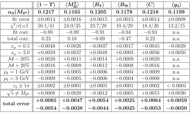
− 0.0054 − 0.0038 − 0.0044 − 0.0025 − 0.0053 − 0.0050 Table 5: Values of α

(M

) are shown from fits of O (α

) QCD predictions combined with power corrections to mean values of 1 − T , M

, B

, B

, C and y

. Statistical and systematic uncertainties are also given. Signs indicate the direction in which α

(M

) changes w.r.t. the standard analysis. The renormalisation and infrared scale uncertainties are added asymmetrically to the errors of α

(M

).

h 1 − T i h M

i h B

i h B

i h C i α

(2 GeV) 0.528 0.663 0.445 0.425 0.461

fit error ± 0.015 ± 0.024 ± 0.020 ± 0.029 ± 0.013 x

= 0.5 +0.002 +0.010 +0.021 +0.118 +0.004 x

= 2.0 − 0.001 − 0.003 − 0.014 − 0.046 − 0.002 M − 20% +0.072 +0.107 +0.055 +0.048 +0.054 M + 20% − 0.049 − 0.072 − 0.037 − 0.032 − 0.037 ε

± 1σ ± 0.002 ± 0.007 ± 0.002 ± 0.002 ± 0.002

√ s 6 = M

− 0.003 +0.017 +0.007 − 0.005 − 0.006 total error +0.074 +0.111 +0.063 +0.131 +0.056

− 0.051 − 0.078 − 0.045 − 0.063 − 0.040

Table 6: Values of α

are shown from fits of O (α

) QCD predictions combined with

power corrections to mean values of 1 − T , M

, B

, B

and C. Statistical and systematic

uncertainties are also given. Signs indicate the direction in which α

changes w.r.t. the

standard analysis.

Figures

1

0 0.1 0.2 0.3 0.4

power correction MC correction

1-T

1

0 0.2 0.4 0.6

power correction MC correction

M

1

0 0.1 0.2 0.3 0.4

power correction MC correction

M

1

0 0.1 0.2 0.3

power correction MC correction

B

1

0 0.05 0.1 0.15 0.2 0.25

power correction MC correction

B

1

0 0.2 0.4 0.6 0.8 1

power correction MC correction

C Figure 1: The figure presents hadronisation correction factors at √

s = 35 GeV estimated

using power corrections (solid lines) or using the JETSET Monte Carlo program (dashed

lines). The hadronisation corrections for power corrections are given by the ratio of the

perturbative QCD prediction over the same prediction combined with power corrections

using the fitted values of α

(M

) and α

(2 GeV). The Monte Carlo hadronisation cor-

rections are given by the ratio of distributions calculated at the parton- and hadron-level,

respectively.

0.2 0.3 0.4 0.5 0.6 0.7 0.8 0.9 1 1.1 1.2

0 0.05 0.1 0.15 0.2 0.25 0.3 0.35

1-T ( σ incl. / σ udsc )(d σ udsc /d σ incl. )

14 GeV 22 GeV 35 GeV 55 GeV

Figure 2: The figure presents ratios of distributions of 1 − T calculated using u, d, s,

and c quarks events or all events using Monte Carlo simulation. The different line types

indicate the cms energy at which the Monte Carlo simulation was run.

1 10 ² 10 ⁴ 10 ⁶ 10 ⁸ 10 ¹⁰ 10 ¹² 10 ¹⁴ 10 ¹⁶ 10 ¹⁸

0 0.1 0.2 0.3

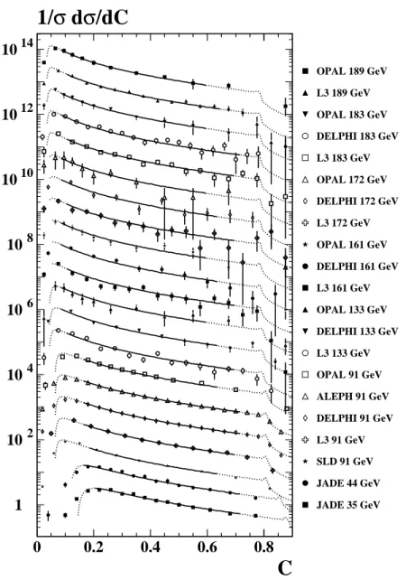
TASSO 14 GeV TASSO 22 GeV HRS 29 GeV MARK2 29 GeV TASSO 35 GeV JADE 35 GeV TASSO 44 GeV JADE 44 GeV AMY 55 GeV SLD 91 GeV L3 91 GeV DELPHI 91 GeV ALEPH 91 GeV OPAL 91 GeV L3 133 GeV DELPHI 133 GeV ALEPH 133 GeV OPAL 133 GeV L3 161 GeV DELPHI 161 GeV OPAL 161 GeV L3 172 GeV DELPHI 172 GeV OPAL 172 GeV L3 183 GeV DELPHI 183 GeV OPAL 183 GeV L3 189 GeV OPAL 189 GeV

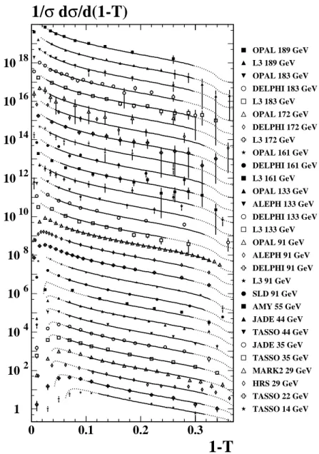
1-T 1/ σ d σ /d(1-T)

Figure 3: Scaled distributions for 1 − T measured at √

s = 14 to 189 GeV. The error

bars indicate the total errors of the data points. The solid lines show the result of the

simultaneous fit of α

(M

) and α

using resummed O (α

)+NLLA QCD predictions with

the ln(R)-matching combined with power corrections. The dotted lines represent an

extrapolation of the fit result.

10

1 10 10

10

10

10

0.1 0.2 0.3 0.4 0.5 0.6

JADE 35 GeV JADE 44 GeV OPAL 91 GeV OPAL 133 GeV OPAL 161 GeV OPAL 172 GeV OPAL 183 GeV OPAL 189 GeV

M

1/ σ d σ /dM

1 10 10

10

10

10

10

10

10

10

10

10

10

0 0.05 0.1 0.15 0.2 0.25

TASSO 14 GeV TASSO 22 GeV TASSO 35 GeV TASSO 44 GeV SLD 91 GeV L3 91 GeV DELPHI 91 GeV ALEPH 91 GeV L3 133 GeV DELPHI 133 GeV L3 161 GeV DELPHI 161 GeV L3 172 GeV DELPHI 172 GeV L3 183 GeV DELPHI 183 GeV L3 189 GeV

M

1/ σ d σ /dM

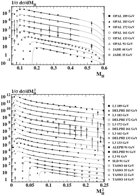
Figure 4: Scaled distributions for M

and M

measured at √

s = 14 to 189 GeV. The

error bars indicate the total errors of the data points. The solid lines show the result of

the simultaneous fit of α

(M

) and α

using resummed O (α

)+NLLA QCD predictions

with the ln(R)-matching combined with power corrections. The dotted lines represent an

extrapolation of the fit result.

1 10 10

10

10

10

10

10

10

10

10

10

10

10

0 0.1 0.2 0.3

B _T 1/ σ d σ /dB _T

0 0.1 0.2 0.3

JADE 35 GeV JADE 44 GeV SLD 91 GeV DELPHI 91 GeV OPAL 91 GeV L3 133 GeV DELPHI 133 GeV OPAL 133 GeV L3 161 GeV DELPHI 161 GeV OPAL 161 GeV L3 172 GeV DELPHI 172 GeV OPAL 172 GeV L3 183 GeV DELPHI 183 GeV OPAL 183 GeV L3 189 GeV OPAL 189 GeV

B _W 1/ σ d σ /dB _W

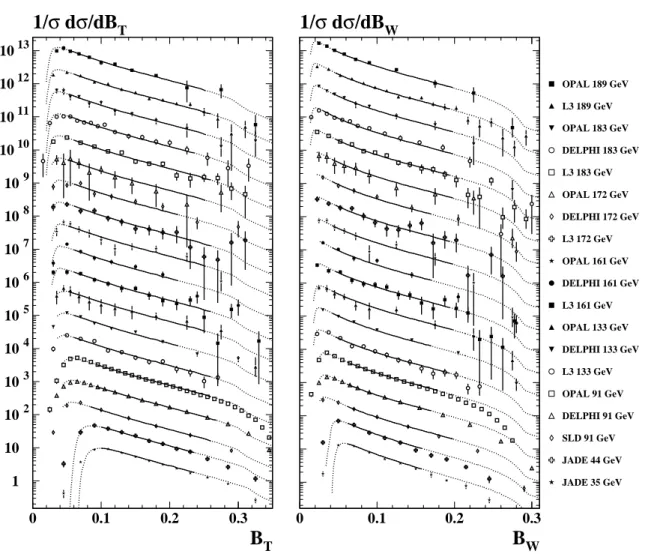
Figure 5: Scaled distributions for B

and B

measured at √

s = 35 to 189 GeV. The

error bars indicate the total errors of the data points. The solid lines show the result of

the simultaneous fit of α

(M

) and α

using resummed O (α

)+NLLA QCD predictions

with the ln(R)-matching combined with power corrections. The dotted lines represent an

extrapolation of the fit result.

1 10 ² 10 ⁴ 10 ⁶ 10 ⁸ 10 ¹⁰ 10 ¹² 10 ¹⁴

0 0.2 0.4 0.6 0.8

JADE 35 GeV JADE 44 GeV SLD 91 GeV L3 91 GeV DELPHI 91 GeV ALEPH 91 GeV OPAL 91 GeV L3 133 GeV DELPHI 133 GeV OPAL 133 GeV L3 161 GeV DELPHI 161 GeV OPAL 161 GeV L3 172 GeV DELPHI 172 GeV OPAL 172 GeV L3 183 GeV DELPHI 183 GeV OPAL 183 GeV L3 189 GeV OPAL 189 GeV

C 1/ σ d σ /dC

Figure 6: Scaled distributions for C measured at √

s = 35 to 189 GeV. The error

bars indicate the total errors of the data points. The solid lines show the result of the

simultaneous fit of α

(M

) and α

using resummed O (α

)+NLLA QCD predictions with

the ln(R)-matching combined with power corrections. The dotted lines represent an

extrapolation of the fit result.

0 0.02 0.04 0.06 0.08 0.1 0.12 0.14 0.16 0.18 0.2

0 20 40 60 80 100 120 140 160 180 200

√⁻⁻s [GeV]

〈1-T〉

Mark J TASSO DELCO Mark II JADE L3 AMY DELPHI ALEPH OPAL SLD

0 0.02 0.04 0.06 0.08 0.1 0.12 0.14

0 20 40 60 80 100 120 140 160 180 200

√⁻⁻s [GeV]

〈MH2/s〉

TASSO Mark II JADE L3 AMY DELPHI OPAL SLD ALEPH

0 0.02 0.04 0.06 0.08 0.1 0.12 0.14 0.16 0.18 0.2

0 20 40 60 80 100 120 140 160 180 200

√⁻⁻s [GeV]

〈BT〉

JADE L3 DELPHI SLD OPAL ALEPH

0 0.02 0.04 0.06 0.08 0.1 0.12 0.14

0 20 40 60 80 100 120 140 160 180 200

√⁻⁻s [GeV]

〈BW〉

JADE L3 DELPHI SLD OPAL ALEPH

0 0.1 0.2 0.3 0.4 0.5

0 20 40 60 80 100 120 140 160 180 200

√⁻⁻s [GeV]

〈C〉

O(α_S²)+Power Corr.

O(α_S²) only JADE L3 ALEPH DELPHI OPAL SLD

0 0.005 0.01 0.015 0.02 0.025 0.03 0.035 0.04

0 20 40 60 80 100 120 140 160 180 200

√⁻⁻s [GeV]

〈y3〉

JADE DELPHI OPAL SLD L3

Figure 7: The energy dependence of h 1 − T i , h M

i , h B

i , h B

i , h C i and h y

i is shown.

The solid curves are the results of fits using perturbative O (α

) QCD calculations com-

bined with power corrections while the dashed lines indicate the contribution from the

perturbative prediction only.