transport to the free troposphere

Meteorological constraints on marine atmospheric halocarbons and their

transport to the free troposphere

Dissertation

zur Erlangung des Doktorgrades

der Mathematisch-Naturwissenschaftlichen Fakultät der Christian-Albrechts-Universität zu Kiel

Vorgelegt von Steffen Fuhlbrügge Kiel, September 2015

iii Zusammenfassung

Zusammenfassung

Mit Inkrafttreten des Montreal-Protokolls in 1989 wurde der globale Ausstoß anthropogener Halogenkohlenwasserstoffe reduziert, was zu einem stärkeren Beitrag natürlich produzierter Halogenkohlenwasserstoffe zum atmosphärischen Halogenhaushalt in der Zukunft führen wird.

Solche natürlichen Halogenverbindungen mit einer mittleren atmosphärischen Lebenszeit von bis zu einem halben Jahr, sogenannte sehr kurzlebige Substanzen (Very Short-Lived Substances, VSLS) beeinflussen die Oxidationsfähigkeit der Troposphäre und Stratosphäre (von Glasow and Crutzen, 2007). Den größten Beitrag zum atmosphärischen Bromgehalt leisten Bromoform und Dibrommethan durch Produktion von Mikro- und Makroalgen (e.g. Quack and Wallace, 2003;Law and Sturges, 2007). Iodmethan (veraltet Methyliodid), welches sowohl von Mikro und Makro-Algen als auch durch photochemische Reaktionen im Oberflächenwasser entsteht, leistet hingegen einen signifikanten Beitrag zum atmosphärischen Iodhaushalt (e.g. Butler et al., 2007;Hughes et al., 2011).

Erhöhte Emissionen dieser VSLS werden vorwiegend in tropischen Ozeanen, ozeanischen Auftriebsgebieten und küstennah beobachtet. Daher spielen diese Regionen eine entscheidende Rolle für den atmosphärischen Halogenhaushalt. In Verbindung mit intensiver tropischer Konvektion können VSLS bis in die obere Troposphäre, bzw. untere Stratosphäre gelangen (Montzka and Reimann, 2011).

Diese Doktorarbeit untersucht den Einfluss meteorologischer Bedingungen und ozeanischer Emissionen auf atmosphärische VSLS Konzentrationen über Ozeanen und deren Transport in die freie Troposphäre. Die Arbeit umfasst drei Schiffskampagnen in verschiedenen ozeanischen und atmosphärischen Regimen: die DRIVE (Diurnal and Regional Variability of halogen Emissions) Kampagne mit FS POSEIDON im tropischen und subtropischen Nordostatlantik im Mai und Juni 2010, die SHIVA (Stratospheric ozone: Halogen Impacts in a Varying Atmosphere) Kampagne mit FS SONNE im tropischen Südchinesischem Meer und der Sulusee im November 2011, sowie der M91 SOPRAN (Surface Ocean Processes in the Antropocene) Kampagne mit FS METEOR im tropischen Südostpazifik im Dezember 2012. Meteorologische Parameter (Temperatur, Wind, Feuchte) wurden von den Schiffssensoren und den Radiosondierungen an Bord während jeder Kampagne gemessen, um atmosphärische Gegebenheiten nahe der Oberfläche, in der marinen atmosphärischen Grenzschicht (Marine Atmospheric Boundary Layer, MABL) und in der freien Troposphäre zu untersuchen. VSLS Proben wurden regelmäßig im Oberflächenwasser und in der marinen Atmosphäre während der Fahrten genommen. Die ersten beiden Manuskripte präsentieren Beobachtungen der DRIVE Kampagne. Manuskript 1 untersucht meteorologische Einflüsse insbesondere der MABL auf atmosphärisches Bromoform, Dibrommethan und Iodmethan, sowie deren tägliche Schwankungen

iv Meteorological constraints on marine atmospheric halocarbons

(Fuhlbrügge et al., 2013), während das zweite Manuskript Einflussfaktoren auf ozeanische Emissionen dieser VSLS über dem mauretanischen Auftrieb auf täglicher und regionaler Basis untersucht (Hepach et al., 2014). Manuskript 3 und 4 werten Beobachtungen während der SHIVA Kampagne im Südchinesischem Meer und in der Sulusee aus. Das dritte Manuskript untersucht den Beitrag von VSLS Emissionen zu beobachteten Mischungsverhältnissen in der MABL und der freien Troposphäre mit Hilfe einer Beitrags-Verlust Abschätzung und FLEXPART Trajektorienberechnungen.

Die aufgrund ozeanischer Emissionen berechneten Mischungsverhältnisse von Bromoform, Dibrommethan und Iodmethan in der MABL und der freien Troposphäre werden mit Flugzeugmessungen in der Region während der SHIVA Kampagne verglichen (Fuhlbrügge et al., 2015b). Manuskript 4 präsentiert VSLS Variationen im Oberflächenwasser, deren ozeanischer Emissionen und atmosphärische Mischungsverhältnisse entlang der Fahrtroute (Sentian et al., 2015).

Die M91 SOPRAN Fahrt im tropischen Südostpazifik ist Teil der Manuskripte 5 und 6. Zur Bestätigung der Hauptergebnisse der DRIVE Kampagne im mauretanischen Auftrieb, untersucht Manuskript 5 ähnliche meteorologische Einflüsse auf ozeanische Emissionen und atmosphärische VSLS im peruanischen Auftrieb. Zusätzlich wird die neu entwickelte Beitrags-Verlust Abschätzung aus Manuskript 4 auf die Beobachtungen während M91 angewandt (Fuhlbrügge et al., 2015a). Das 6.

Manuskript konzentriert sich auf den Beitrag iodierter Verbindungen aus ozeanischen Emissionen auf atmosphärische Konzentrationen, sowie deren Transport in die Troposphäre (Hepach et al., 2015, to be submitted).

Zusammenfassend wurden folgende neue Ergebnisse erzielt: Die Auftriebsgebiete entlang der mauretanischen und peruanischen Küsten wurden als Quellregionen für atmosphärisches Bromoform, Dibrommethan und Iodmethan ermittelt. Erhöhte atmosphärische Mischungsverhältnisse dieser Verbindungen wurden küstennah, insbesondere aber über dem ozeanischen Auftrieb in beiden Regionen beobachtet. Meteorologische Faktoren, wie die MABL Eigenschaften zeigten einen signifikanten Einfluss auf die ozeannahen atmosphärischen Mischungsverhältnisse der VSLS und deren ozeanischen Emissionen. Abhängig von der Höhe und Stabilität der MABL sowie der Passatinversion führten die VSLS Emissionen zu einer Anreicherung der Konzentrationen in der untersten Atmosphäre. Die resultierenden geringen Konzentrationsgradienten dämpften die ozeanischen Emissionen und führten zu geringen Schwankungen der VSLS Konzentrationen. Die mit den VSLS angereicherten Luftmassen blieben unterhalb der Inversionsschicht(en) und wurden vorwiegend horizontal und bodennah transportiert.

In Regionen konvektiver Aktivität können die Luftmassen dann in die obere Troposphäre und Tropopause transportiert werden. Als Gegenbeispiel zeigten sich im Südchinesischem Meer und in der Sulusee trotz hoher ozeanischer Konzentrationen und Emissionen relativ geringe VSLS Konzentrationen bodennah und in der MABL. Hier sorgte eine konvektive, instabile MABL und

v Zusammenfassung

tropische Konvektion für einen schnellen Transport von Bodenluft in die freie Troposphäre und einer schnellen Verteilung ozeanischer Emissionen innerhalb dieser. Dieser schnelle vertikale Transport wurde als Grund für die beobachteten geringen MABL VSLS Mischungsverhältnisse identifiziert.

Bromoform in der freien Troposphäre über dem Südchinesischem Meer und der Sulusee stammte nahezu vollständig aus dem örtlichen Südchinesischem Meer, während Dibrommethan und Iodmethan hingegen größtenteils von den Küsten Borneos und den Philippinen sowie des Westpazifiks advehiert wurden.

vii Abstract

Abstract

Emissions of anthropogenic halocarbons have decreased since the commencement of the Montreal Protocol in 1989, which leads to a stronger contribution of naturally produced halocarbons to the atmospheric halogen budget in future. Natural halocarbons with a mean atmospheric lifetime of up to 0.5 years, the so-called Very Short-Lived Substances (VSLS) are known to alter the tropospheric and stratospheric oxidation capacity (von Glasow and Crutzen, 2007). Large contributors of atmospheric bromine are bromoform and dibromomethane, both emitted by micro and macro algae (e.g. Quack and Wallace, 2003;Law and Sturges, 2007). A significant contributor to atmospheric iodine is methyl iodide, which is in addition to micro and macro algae also produced by photochemical reactions in the surface water (e.g. Butler et al., 2007;Hughes et al., 2011). Elevated oceanic emissions are observed in tropical oceans along coasts and above oceanic upwelling. Thus, these regions play a crucial role for the atmospheric halogen budget. In combination with deep tropical convection, the VSLS emissions can be transported into the upper troposphere and lower stratosphere (Montzka and Reimann, 2011).

This thesis investigates the influence of meteorological conditions and oceanic emissions on atmospheric VSLS abundances above the oceans and their transport into the free troposphere during three ship campaigns in different oceanic and atmospheric regimes: the DRIVE (Diurnal and Regional Variability of halogen Emissions) campaign with R/V POSEIDON in the tropical and subtropical Northeast Atlantic during May and June 2010, the SHIVA (Stratospheric ozone: Halogen Impacts in a Varying Atmosphere) campaign with R/V SONNE in the tropical South China and Sulu Seas in November 2011, and the M91 SOPRAN (Surface Ocean Processes in the Antropocene) campaign with R/V METEOR in the tropical Southeast Pacific in December 2012. Meteorological data (e.g.

temperature, wind, humidity) were measured from ships sensors and by radiosonde launches from the ships during each campaign to investigate atmospheric conditions near the surface, in the marine atmospheric boundary layer (MABL) and in the free troposphere. VSLS were regularly sampled in the surface water and in the marine atmosphere during the cruises. The first two manuscripts present results from observations during DRIVE. Manuscript 1 investigates meteorological impacts on atmospheric bromoform, dibromomethane and methyl iodide and their diurnal variability (Fuhlbrügge et al., 2013), while the second manuscript investigates drivers of oceanic emissions of these VSLS above the Mauritanian upwelling on a diel and regional basis (Hepach et al., 2014).

Manuscripts 3 and 4 evaluate observations during SHIVA in the South China and Sulu Seas. The third manuscript investigates the contribution of VSLS emissions to observed MABL and free tropospheric

viii Meteorological constraints on marine atmospheric halocarbons

abundances by developing a source-loss estimate using FLEXPART trajectories. Computed MABL and free troposphere mixing ratios of bromoform, dibromomethane and methyl iodide from the oceanic emissions in the region are compared to SHIVA aircraft observations (Fuhlbrügge et al., 2015b).

Manuscript 4 presents variations of VSLS in the surface water, oceanic emissions and atmospheric abundances along the cruise track (Sentian et al., 2015). The M91 SOPRAN cruise in the Southeast Pacific is part of manuscripts 5 and 6. To evaluate the major findings achieved during the DRIVE campaign at the Mauritanian upwelling, manuscript 5 investigates similar meteorological constraints on oceanic emissions and atmospheric VSLS in the Peruvian upwelling. In addition the new source- loss estimate developed in manuscript 4 is applied to the observations during the M91 cruise (Fuhlbrügge et al., 2015a). The 6th manuscript concentrates on the contribution of iodinated compounds from oceanic emissions to atmospheric abundances and their transport to the troposphere (Hepach et al., 2015, to be submitted).

Overall the following results were achieved. The upwelling regions along the Mauritanian and Peruvian coasts were identified to be medium source regions for atmospheric bromoform, dibromomethane and methyl iodide. Elevated atmospheric mixing ratios of these compounds were found towards the coasts especially above the oceanic upwelling in both regions. Meteorological factors, in particular the MABL characteristics, were identified to impact the atmospheric VSLS mixing ratios and the oceanic emissions significantly. Depending on the height and stability of the MABL as well as the trade inversion, VSLS from oceanic emissions led to an accumulation within the lowermost atmosphere. The resulting low concentration gradients dampened the oceanic emissions and led to minor variations of the marine atmospheric abundances. The VSLS enriched air masses stayed below the inversion layer(s) and were mainly transported horizontally. Within convective activity they could be lifted to the upper troposphere and tropopause. On the opposite, VSLS abundances at the surface and in the MABL were relatively low at coastal regions of the South China and Sulu Seas, despite the high elevated oceanic concentrations and emissions in this area. Here, a convective instable MABL and deep tropical convection led to a rapid exchange of surface air to the free troposphere and a fast distribution of oceanic emissions within the free troposphere. The rapid vertical transport was identified to explain the observed low MABL VSLS mixing ratios. Free tropospheric abundances of bromoform above the South China and Sulu Seas were shown to origin almost entirely from the local South China Sea, while dibromomethane and methyl iodide in contrast were found to be largely advected from the coast of Borneo and the Philippines and from the open West Pacific.

ix Manuscript overview

Manuscript overview

This thesis is based on the following manuscripts:

1. Manuscript: Fuhlbrügge S., Krüger K., Quack B., Atlas E., Hepach H. and Ziska F.: “Impact of the marine atmospheric boundary layer conditions on VSLS abundances in the eastern tropical and subtropical North Atlantic Ocean”, Atmospheric Chemistry and Physics, 13, 6345-6357, 10.5194/acp-13-6345-2013, published 2013.

1.1. Contribution: The results of the manuscript are partly based on the Diploma thesis “Analysis of atmospheric VSLS measurements during the DRIVE campaign in the tropical East Atlantic”

by S. Fuhlbrügge. For the ACP publication, data and figures in the manuscript have been intensively revised and complimented with new results by S. Fuhlbrügge. The manuscript was written by S. Fuhlbrügge. K. Krüger and B. Quack provided input for the preparation and revision of the manuscript. H. Hepach computed the VSLS sea-air fluxes and wrote section 3.4. F. Ziska took atmospheric samples and launched the radiosondes during the DRIVE cruise. E. Atlas analysed the atmospheric VSLS samples.

2. Manuscript: Hepach H., Quack B., Ziska F., Fuhlbrügge S., Atlas E., Krüger K., Peeken I., and Wallace D. W. R.: “Drivers of diel and regional variations of halocarbon emissions from the tropical North East Atlantic”, Atmospheric Chemistry and Physics, 14, 1255-1275, doi:10.5194/acp-14-1255-2014, published 2014.

2.1. Contribution: H. Hepach measured the halocarbons in the sea surface water, evaluated the data, carried out the calculations, and wrote the manuscript. B. Quack contributed to the manuscript preparation and the review process. F. Ziska took air samples and launched radiosondes during the DRIVE cruise. S. Fuhlbrügge analysed and evaluated the meteorological data. E. Atlas measured the atmospheric VSLS samples. I. Peeken measured and calculated the phytoplankton pigments. F. Ziska, S. Fuhlbrügge, E. Atlas, I. Peeken, K.

Krüger and D. W. R. Wallace helped revising the manuscript.

x Meteorological constraints on marine atmospheric halocarbons

3. Manuscript: Fuhlbrügge S., Quack, B., Tegtmeier, S., Atlas, E., Hepach, H., Shi, Q., Raimund, S., and Krüger, K.: “The contribution of oceanic very short lived halocarbons to marine and free troposphere air over the tropical West Pacific”, Atmospheric Chemistry and Physics Discuss., 15, 17887-17943, doi:10.5194/acpd-15-17887-2015, published for discussion 2015.

3.1. Contribution: S. Fuhlbrügge and K. Krüger took atmospheric samples and launched radiosondes during the SHIVA cruise. S. Fuhlbrügge analysed the data, developed the methodologies and wrote the manuscript. K. Krüger and B. Quack assisted with the campaign preparation and post-processing, and provided input during the preparation of the manuscript. S. Tegtmeier calculated the FLEXPART runs and provided helpful comments during the preparation of the manuscript. E. Atlas analysed the atmospheric VSLS samples.

H. Hepach, Q. Shi and S. Raimund measured halocarbons in the sea surface water.

4. Manuscript: Sentian J., Xiang, C. T., Jing, H. C., Quack, B., Fuhlbrügge, S., Krüger, K., and Atlas, E.:

“Observation of the Variations of Very Short-Lived Halocarbon Emissions in Tropical Coastal Marine Boundary Layer”, Advanced Science Letters, 21, 144-149, doi:10.1166/asl.2015.5856, published 2015.

4.1. Contribution: S. Fuhlbrügge and K. Krüger took the atmospheric VSLS samples during the SHIVA cruise. E. Atlas analysed the atmospheric VSLS samples. J. Sentian wrote the manuscript. B. Quack took the water samples and computed the VSLS sea-air fluxes.

5. Manuscript: Fuhlbrügge, S., Quack B., Atlas E., Fiehn A., Hepach H., Krüger K.: “Meteorological constraints on oceanic halocarbons above the Peruvian Upwelling”, Atmospheric Chemistry and Physics Discuss., 15, 20597-20628, doi:10.5194/acpd-15-20597-2015, published for discussion 2015.

5.1. Contribution: S. Fuhlbrügge took the atmospheric VSLS samples and launched radiosondes during the M91 cruise, analysed the data, and wrote the manuscript. K. Krüger and B. Quack assisted with the campaign preparation and post-processing, and provided input during the preparation of the manuscript. E. Atlas analysed the atmospheric VSLS samples. A. Fiehn calculated the FLEXPART runs. H. Hepach measured halocarbons in the sea surface water.

xi Manuscript overview

6. Manuscript: Hepach H., Quack B., Tegtmeier S., Engel A., Bracher A., Fuhlbrügge S. , Galgani L., Raimund S., Atlas E., Lampel J. und Krüger K.: “Biogenic halocarbons from the Peruvian upwelling as tropospheric halogen source”, to be submitted.

6.1. Contribution: H. Hepach measured the halocarbons in surface water, calculated iodocarbon fluxes and wrote the manuscript. B. Quack helped writing the manuscript, interpreted the data and provided input during the correction of the manuscript. S. Tegtmeier calculated the contributions of organoiodine to IO and provided input during the correction of the manuscript. A. Engel and L. Galgani measured DOM in the SML and the subsurface and helped interpreting the data. A. Bracher provided the phytoplankton measurements and helped correcting the manuscript. S. Fuhlbrügge took the air samples and provided input during manuscript preparation. S. Raimund measured the halocarbon in the depth profiles.

E. Atlas measured the atmospheric samples. J. Lampel was responsible for IO data onboard RV Meteor. K. Krüger helped correcting the manuscript.

xiii Content

Content

Zusammenfassung ... iii

Abstract ... vii

Manuscript overview ... ix

Content ... xiii

1. Introduction ...1

1.1 Halocarbons ...1

1.2 Very Short-Lived Substances (VSLS) ...2

1.2.1 Marine sources ...2

1.2.2 Sea-air gas exchange ...3

1.2.3 Sea-air flux parameterization ...4

1.2.4 Tropospheric abundances ...6

1.3 The Marine Atmospheric Boundary Layer (MABL) ...8

1.3.1 MABL height determination from radiosoundings ... 10

1.3.2 Transport modelling ... 11

1.4 VSLS study regions ... 12

1.4.1 Oceanic upwelling in the Northeast Atlantic and the Southeast Pacific ... 12

1.4.2 The South China and Sulu Seas in the tropical West Pacific ... 13

2. Thesis outline ... 15

3. Results ... 17

3.1 Manuscript 1 ... 17

3.2 Manuscript 2 ... 33

3.3 Manuscript 3 ... 57

3.4 Manuscript 4 ... 89

3.5 Manuscript 5 ... 97

3.6 Manuscript 6 ... 115

4. Synthesis and Outlook ... 147

5. Bibliography ... 151

6. Lists... 163

6.1 Figures... 163

6.2 Tables ... 165

Danksagung ... 167

Eidesstattliche Erklärung ... 169

xiv Meteorological constraints on marine atmospheric halocarbons

1 Introduction

1. Introduction

Atmospheric halogenated trace gases from natural sources play a significant role in the oxidation capacity of the troposphere and stratosphere (e.g. von Glasow and Crutzen, 2007;Simpson et al., 2015). They also contribute to the atmospheric halogen loading and to the ozone budget. For example natural halocarbons from the ocean contribute up to 25 % to the halogen burden in the stratosphere (Dorf et al., 2006) and significantly deplete ozone there (Salawitch et al., 2005;Sinnhuber and Folkins, 2006;Yang et al., 2014). To estimate the global contribution of natural halocarbons, marine and atmospheric observations were investigated during various measurement campaigns around the globe (e.g. Quack and Suess, 1999;Carpenter et al., 2007;Brinckmann et al., 2012). Surface observations of these natural halocarbons were taken in the atmospheric boundary layer and their abundance thus may be influenced by meteorological conditions there such as the extent and condition of the boundary layer. The investigation of these natural halocarbons and their transport pathways in the lower atmosphere will help to identify source regions and hot spots in the ocean and help to evaluate the contribution of source regions to atmospheric abundances. This thesis concentrates on three halocarbons with natural sources in the oceans: Methyl iodide, an important carrier of iodine to the atmosphere (Saiz-Lopez et al., 2012) as well as bromoform and dibromomethane, which are the largest natural contributors to atmospheric bromine (Penkett et al., 1985;Quack and Wallace, 2003;Hossaini et al., 2012).

1.1 Halocarbons

The collective term ‘halocarbon’ refers to a broad spectrum of hydrocarbons in which at least one carbon atom is linked covalently to one or more halogen atoms, e.g. fluorine, chlorine, bromine or iodine. Anthropogenic halocarbons containing chlorine and fluorine, the so called chlorofluorocarbons (CFCs) and those containing bromine, the so called halons, were widely used as propellants, fire extinguishants, refrigerants and solvents since the 1930s. The careless emissions and the inert characteristic of these anthropogenic halocarbons led to an accumulation of these compounds in the atmosphere, which was first reported by Lovelock (1971) and by Lovelock and Maggs (1973). Solar radiation in the stratosphere can release halogen radicals from these halocarbons. The radicals are then involved in catalytic ozone cycles, leading to ozone loss in the stratosphere. Although this reaction was already suggested by Molina and Rowland (1974), it was not generally accepted in the scientific community until the discovery of the Antarctic ozone hole by

2 Meteorological constraints on marine atmospheric halocarbons

Chubachi (1984) and Farman et al. (1985). With the commencement of the Montreal Protocol in January 1989 the signatory states committed a reduction down to a fully abolition of anthropogenic halocarbon emissions. Indeed, a decrease of the atmospheric halocarbon abundances and a slow recovery of the stratospheric ozone layer were observed in the last years (Pawson and Steinbrecht, 2015). The very long atmospheric lifetimes of certain halocarbons, e.g. CFC-11 with 52 years and CFC- 12 with 102 years, lead to a delayed reduction of these compounds in the atmosphere (Pawson and Steinbrecht, 2015). With the decline of anthropogenic halocarbon emissions, naturally produced halocarbons and their contribution to the atmospheric halogen load moved further into the scientific focus (Ko and Poulet, 2003). In particular global climate changes e.g. sea surface temperature and wind speed changes, are expected to affect oceanic emissions of these halocarbons (Ziska et al., 2013). If the lifetime of a natural halocarbon exceeds transport timescales in the troposphere, it can be transported into the stratosphere, e.g. due to deep convection in the tropics (Montzka and Reimann, 2011). To estimate current and future halocarbon emissions from natural sources and their transport pathways in the atmosphere it is fundamental to investigate and identify present halocarbon source regions and their particular contribution to the atmospheric halogen loading.

Therefore this thesis presents new unpublished halocarbon observations to improve global halocarbon climatologies, develops a method to estimate the contribution of natural halocarbons emissions to the observed boundary layer and free troposphere abundances, and investigates the meteorological constraints especially of boundary layer conditions on marine halocarbon abundances.

1.2 Very Short-Lived Substances (VSLS)

Halogenated trace gases with local tropospheric lifetimes of less than 6 months and mainly natural sources have been summarized as Very Short-Lived Substances (VSLS) and can significantly contribute to the atmospheric halogen load (Ko and Poulet, 2003;Dorf et al., 2006;Law and Sturges, 2007;Montzka and Reimann, 2011).

1.2.1 Marine sources

VSLS sources mainly origin from the ocean. Marine abundances of bromoform and dibromomethane are known to originate from biotic sources. The production of both compounds in the open ocean is attributed predominantly to phytoplankton (Fogelqvist, 1985;Class and Ballschmiter, 1988;Moore

3 Introduction

and Tokarczyk, 1993;Quack and Wallace, 2003). In coastal regions, macro algae such as brown, green and red algae are known to be dominant producers of oceanic bromoform and dibromomethane (Gschwend et al., 1985;Nightingale et al., 1995;Quack et al., 2004;Law and Sturges, 2007). Methyl iodide can be produced by algae and phytoplankton (Hughes et al., 2011;Manley and Dastoor, 1988;Manley and de la Cuesta, 1997), as well as abiotic due to photochemical processes in surface sea water (Butler et al., 2007;Chuck et al., 2005;Happell and Wallace, 1996;Moore and Zafiriou, 1994).

1.2.2 Sea-air gas exchange

Brominated and iodinated VSLS are predominantly emitted from the ocean. Known global emissions range from 116 – 820 Gg Br yr^-1 for bromoform, 57 – 280 Gg Br yr^-1 for dibromomethane and 157 – 550 Gg I yr^-1 for methyl iodide (Table 1-1). While the majority of studies reveal a significantly higher contribution of coastal emissions to global emissions for bromoform with up to 81 %, dibromomethane and methyl iodide are mainly emitted from the open ocean with up to 78 %, respectively 89 % (Ziska et al., 2013). Although these estimates reveal large uncertainties due to the high spatial and temporal variability of the oceanic emissions, different emission estimates (top- down versus bottom-up approaches) and limited input data, elevated emissions are generally found in tropical regions (Yokouchi et al., 2005;Montzka and Reimann, 2011). While top-down estimates reproduce oceanic emissions via a synchronization of atmospheric VSLS-data with simulations of chemistry climate models, bottom-up estimates take surface measurements to compute air-sea fluxes directly. Ziska et al. (2013) were the first who established and used a database of worldwide halogenated VSLS observations (HalOcAt, https://halocat.geomar.de/de) for their bottom-up estimates. Since they used the highest number of available observations, their computed oceanic fluxes appear most reliable. However, the data base is very sparse which reveals the need for further observations to investigate the variability of the oceanic emissions und to improve these estimates.

VSLS observations of the first and second manuscript (DRIVE) are already included in the HalOcAt database, which was used for the Ziska climatology (Ziska et al., 2013). Measurements of the remaining manuscripts (3 - 6) are planned to be integrated into the HalOcAt database for future global VSLS climatologies.

4 Meteorological constraints on marine atmospheric halocarbons

1.2.3 Sea-air flux parameterization

Direct flux measurement techniques of bromoform, dibromomethane and methyl iodide are still in development and testing. To investigate the sea-air gas exchange of these compounds, their fluxes are parameterized. Generally, a flux F between two fluids can be described after Eq. 1, with k as a transfer coefficient and ∆c as the concentration gradient between the two fluids:

(Eq. 1)

Liss and Slater (1974) were the first to present a simple two-layer model of a flat gas-liquid interface (Figure 1-1). Assuming the gas film to obey the solubility of a gas in a liquid after Henry’s Law and the main resistance occurring at the transfer through the specific gas/liquid film, Eq. 1 can be transformed into Eq. 2, with kl as the transfer coefficient for the liquid, H as the Henry’s Law coefficient that varies

Table 1-1: Oceanic emissions of bromoform and dibromomethane in Gg Br yr^-1, and methyl iodide in Gg I yr^-1. Coast includes shelf estimates. Studies using a bottom-up approach are marked by ↑, top- down by ↓ and model studies by ○. Ziska et al. (2013) uses 2 different methods, robust fit (RF) and ordinary least squares (OLS).

Reference

Bromoform Dibromomethane Methyl iodide Global Open

Ocean Coast Global Open

Ocean Coast Global Open

Ocean Coast

Bell et al. (2002) ○ 305

Quack and W. (2003) ↑ 800 241 559 Yokouchi et al. (2005) ↑ 820

Warwick et al. (2006) ↓ 560 280 280 100

Butler et al. (2007) ↑ 800 150 650 280 50 230 550 270 280

Kerkweg et al. (2008) ↓ 596 113

Carpenter et al. (2009) ↑ 200

O’Brien et al. (2009) ↑ 820 Palmer et al. (2009) ↑ 116

Liang et al. (2010) ↓ 430 260 170 57 34 23

Pyle et al. (2011) ↓ 382 100

Ordonez et al. (2012) ↓ 533 67 213

Ziska et al. (2013) OLS ↑ 199 50 149 78 61 17 184 163 21

Ziska et al. (2013) RF ↑ 120 30 90 62 48 14 157 137 20

5 Introduction

with temperature and salinity, cg as the concentration in the gas and cl as the concentration in the liquid. In case of a low solubility of a gas in the liquid, Eq. 2 can be used to calculate the net flux (Nightingale, 2009).

However, diffusion in the molecular

layers can only be estimated which means the transfer coefficient kl has to be parameterized.

(Eq. 2)

Since various factors are known to influence the sea-air flux, e.g. wind speed, turbulence, heat flux, and mixing depths, the range of known transfer coefficients reveals the complexity of considering all these factors (Wanninkhof et al., 2009;Garbe et al., 2014). To describe the viscosity of a gas in water, the Schmidt number Sc (Table 1-2) is used, which is defined as the ratio of momentum diffusivity (ϑ) to the diffusivity for mass transfer. The estimation of the transfer coefficients kl for bromoform, dibromomethane and methyl iodide is based on a power law dependence of the parameterization by Nightingale (2009), which lies well in range of known transfer coefficients and is expressed for a Schmidt number of 600 for CO2 at 20 °C in fresh water (Eq. 3) with u10 as a 10 minute wind speed mean at 10 m height.

(Eq. 3) The specific diffusion coefficients can then be computed after Eq. 4 (Quack and Wallace, 2003), which leads to the final equation for the net sea-air flux (Eq. 5).

Table 1-2: Schmidt numbers (ScVSLS) and Henry’s Law coefficient (HVSLS) for bromoform, dibromomethane and methyl iodide with T as liquid temperature (Hayduk and Laudie, 1974;Wilke and Chang, 1955;Sander, 1999;Moore et al., 1995a;Moore et al., 1995b;Quack and Wallace, 2003).

VSLS ScVSLS HVSLS

Bromoform

(

) Dibromomethane

(

) Methyl iodide

(

) Figure 1-1: Two-layer model of sea-air gas exchange through an interface. Adopted from Liss and Slater (1974).

6 Meteorological constraints on marine atmospheric halocarbons

(Eq. 4)

(Eq. 5)

The fluxes of bromoform, dibromomethane and methyl iodide are used in order to estimate the contribution of oceanic emissions to atmospheric abundances.

1.2.4 Tropospheric abundances

The increasing number of atmospheric surface halogenated VSLS data points around the globe during the last decades helped to improve global VSLS climatologies (e.g. Warwick et al., 2006;Ziska et al., 2013) (Figure 1-2). Elevated mixing ratios of most brominated VSLS are found predominantly in coastal regions and in the tropics due to elevated oceanic emissions in these areas (Section 1.2.2). In tropical regions, the VSLS and their product gases can be transported by (deep) convection into higher altitudes when their atmospheric lifetimes are longer than transport processes in the atmosphere (Quack et al., 2004;Salawitch, 2006;Aschmann et al., 2009;Aschmann et al., 2011;Ashfold et al., 2012). The atmospheric lifetimes of bromoform, dibromomethane and methyl iodide are governed by several chemical reactions, once they are emitted into the atmosphere. Both, bromoform and dibromomethane are degraded by photolysis and hydroxyl radicals (OH) (Figure 1-3). A source for OH radicals in the troposphere is ozone (O3). Although about 90 % of global ozone is found in the stratosphere, tropospheric ozone acts as a toxic pollutant and greenhouse gas (Crutzen, 1971;Reeves et al., 2002;Weinhold, 2008;Stevenson et al., 2013).

Figure 1-2: Global maps of atmospheric surface mixing ratios [ppt] of bromoform (CHBr3), dibromomethane (CH2Br2) and methyl iodide (CH3I) computed by Ziska et al. (2013)

7 Introduction

Figure 1-3: Tropospheric degradation scheme of bromoform (CHBr3) and dibromomethane (CH2Br2) after Hossaini et al. (2010). Organic species are shown in red boxes, fast reactions are given by blue lines and the production of Bry is given by dashed lines.

While bromoform is predominantly degraded by photolysis, dibromomethane is mainly degraded by reactions with OH. Estimates on the atmospheric lifetimes of bromoform and dibromomethane in the tropics have strongly varied during the past (McGivern et al., 2002;Ko and Poulet, 2003;McGivern et al., 2004;Law and Sturges, 2007). Most recent studies reveal a mean lifetime for bromoform of 15 days in the MABL and 17 days in the entire troposphere, respectively 94 days and 150 days for dibromomethane (Carpenter and Reimann, 2015). The major primary oxidation products of bromoform are carbonyl bromide (CBr2O) and formyl bromide (CHBrO), latter is also the major degradation product of dibromomethane. These compounds furthermore release HBr, HOBr and BrO, summarized as Bry due to photolysis as reactive bromine, which has been shown to be 60 times more effective in ozone destruction than chlorine (Montzka and Reimann, 2011). Von Glasow (2004) and Yang et al. (2005) simulated a decrease of the tropospheric ozone by 5 to 30 % when considering bromine in the troposphere. Chemical degradation of methyl iodide in the MABL and free troposphere is even faster with a mean lifetime of 3, respectively 4 days (Carpenter and Reimann, 2015). It is rapidly photolyzed into inorganic iodine (Iy). Once Bry and Iy are released into the atmosphere they enter catalytic reaction cycles with ozone (O3). Catalytic key reactions in the troposphere involving halogen oxidation and halogen oxide self-reactions are (Read et al., 2008):

8 Meteorological constraints on marine atmospheric halocarbons

(R2.1)

(R1.1) (R2.2)

(R1.2) (R2.3)

net: (R1.3) net: (R2.4)

Here, X and Y are representative for halogen radicals, either bromine (Br), or iodine (I) (or chlorine, Cl). They react within seconds with ozone and produce halogen oxides (XO, YO). The halogen radicals can also suppress ozone formation by perturbing HO2/OH ratios (von Glasow et al., 2004):

(R3.1)

(R3.2)

Saiz-Lopez et al. (2014) estimated the integrated contribution of catalytic iodine reactions to the total rate of tropospheric ozone loss to be up to 5 times larger than the combined bromine and chlorine cycles.

1.3 The Marine Atmospheric Boundary Layer (MABL)

For surface trace gas observations it is fundamental to investigate the stability and structure of the lowermost atmosphere, which usually extends from the surface up to about 3 km height.

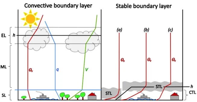
Atmospheric constituents such as gases and aerosols emitted into the MABL are gradually dispersed before they are completely mixed within approximately one hour in the MABL due to turbulence and convection (Stull, 1988;Holton and Hakim, 2012). However, under stable conditions in the MABL complete mixing is often not fully reached (Seibert et al., 2000). MABL conditions can be observed by direct measurements (e.g. radiosondes, tethered balloons, weather masts, and aircrafts) and by remote sensing techniques (e.g. Doppler weather radars, LiDAR and SODAR). Two different kinds of MABLs exist (Figure 1-4), the convective boundary layer (CBL) and the stable boundary layer (SBL).

The CBL consists of a surface layer (SL), which extents up to 100 m height and is strongly influenced by the Earth’s surface, e.g. heating or cooling of the surface, evaporation and friction. Above lies the so-called mixed layer (ML) in which compounds are vertically well mixed. In the SL and ML, mixing occurs due to turbulence. The transition from the ML to the free troposphere is called entrainment layer (EL), where turbulence and vertical transport declines towards the top. In this thesis, the MABL height in case of a convective boundary layer is chosen as the centre of the EL. The SBL can also be split into two layers, a lower layer of continuous turbulence (CTL) and a layer of sporadic

9 Introduction

turbulence (STL) above. In case of low wind speeds and a strong stability of the lower atmosphere the STL can even extent to the ground and lead to very low boundary layer heights and thus a very small volume of air in which compounds are mixed (Figure 1-4, right side). With increase of the wind speed in the CTL, turbulence leads to an increase of the MABL height (b, c) (Seibert et al., 2000). In this thesis, CBL and SBL are investigated above different oceanic regimes by radiosonde launches.

Major foci are mixing of trace gases within the MABL and the transport of surface air masses out of the MABL into the free troposphere under convective and stable MABL conditions. These require the determination of the MABL height and condition as well as the computation of trajectories to estimate the timescales of surface air remaining in the MABL, respectively leaving the MABL.

Figure 1-4: Exemplary profiles of convective (left) and stable (right) boundary layers (Stull, 1988;Seibert et al., 1997, 2000); virtual potential temperature (Θv, red), humidity (q, blue) and wind speed (V, green). The height of the boundary layer is given by h, the Surface Layer by SL, the Mixed Layer by ML, the Entrainment Layer by EL, the Continuously Turbulence Layer by CTL, and the Sporadic Turbulence Layer by STL. The height of the SBL varies with the height of the STL: (a) STL reaches the surface, (b) and (c) a CTL leads to an increase of the SBL height.

10 Meteorological constraints on marine atmospheric halocarbons

1.3.1 MABL height determination from radiosoundings

The height of the MABL determines the available volume in which compounds are rapidly mixed and is therefore an essential parameter e.g. for air pollution studies. Unfortunately, it is a rather unspecific meteorological quantity, with different definitions and estimations (Stull, 1988;Garratt, 1990;Seibert et al., 2000). In this thesis, the MABL is investigated by radiosonde observations.

Definitions and characteristics of the MABL as well as methods to determine its height are adopted from Seibert et al. (2000). The MABL height can be determined from radiosonde derived atmospheric profiles of temperature, humidity and wind. With this data it can be derived objectively and subjectively. Objective methods include e.g. the Holzworth method (Holzworth, 1964, 1967, 1972), which basically starts at the surface with the measured temperature and follows the dry adiabate up to the point of intersection with the temperature of the most recent radiosounding. However, this method strongly depends on the surface temperature and thus results in high uncertainties of the estimated MABL height (Aron, 1983, 1985). Another objective method is the computation of the bulk Richardson number Rib (Troen and Mahrt, 1986;Vogelezang and Holtslag, 1996). It is a dimensionless number that relates the vertical stability to the vertical shear, respectively the thermally produced turbulence to shear induced turbulence, which makes it only suitable for unstable convective conditions (Seibert et al., 2000). Rib is computed at the height z from radiosonde measurements after Eq. 6 with g as the acceleration of gravity, Θv(z) as the virtual potential temperature at level z, Θv1 as the virtual potential temperature at ground level, U(z) as the zonal wind at level z and V(z) as the meridional wind at level z. If Rib reaches a critical value of 0.25, z(Rib ≥ 0.25) defines the height of the MABL (Sørensen et al., 1996).

(Eq. 6)

The potential temperature Θ describes the temperature of an air parcel that is lifted adiabatically to a surface pressure level p (von Bezold, 1888). In case of condensation and evaporation Θ is replaced by the virtual potential temperature Θv.

Besides this objective method the MABL height can be determined subjectively from the radiosoundings as well. Here, the temperature, humidity and wind profiles of the lower troposphere are used to identify stable layers under convective conditions. These stable layers, e.g. a temperature inversion, often coincide with significant reductions of humidity and wind shear (Seibert et al., 2000).

Since the identification of stable layers in temperature profiles is not always straight forward, Θv can be used instead of the air temperature (Stull, 1988). Here, in case of a CBL, a decrease of Θv reveals

11 Introduction

unstable atmospheric conditions, a constant Θv neutral atmospheric conditions and an increase of Θv

the beginning of a stable layer (Figure 1-4). Stull (1988) suggested to take the base of the stable layer increased by half of the stable layer depth as the MABL height. Under SBL conditions, the stable layer can even reach the surface. In this case the MABL height depends on sporadic turbulence and can therefore be distinguished from vertical wind shear which influences the vertical gradient of Θv

(Figure 1-4, SBL case: a, b, c).

1.3.2 Transport modelling

The transport timescale of MABL air into the free troposphere in thises were determined from the residence time of surface trajectories below the determined MABL height. These trajectories were computed with the Lagrangian Particle Dispersion Model FLEXPART, developed at the Norwegian Institute for Air Research in the Department of Atmospheric and Climate Research (Stohl et al., 2005). The model includes various parameterizations, e.g. for boundary layer and free troposphere turbulence and moist convection (Stohl and Thomson, 1999;Forster et al., 2007). 6-hourly meteorological input fields from the assimilation reanalysis product ERA-Interim (Dee et al., 2011) were used, including air temperature, boundary layer height, horizontal and vertical wind, humidity and convective, respectively large scale precipitation with a spatial resolution of 1° x 1° at 60 vertical levels up to 0.1 hPa. Except for the DRIVE ship campaign, radiosonde observations were instantly uploaded and assimilated into the Global Telecommunication System (GTS) to improve the accuracy of the ERA-Interim meteorological input fields for our investigations. For the investigation of the air mass transport, 10,000 trajectories were launched along the cruise tracks during SHIVA and M91. The release events were synchronized with the sampling of atmospheric and surface ocean data on the ships and performed within a time frame of ± 30 minutes and an area of 400 m² around the measurement locations. The time, these trajectories needed to exceed the determined MABL height was then related to the contribution of oceanic emissions to the MABL air content of the three investigated VSLS. In this mass balance calculation, the oceanic delivery acted against the loss of trajectories out of the MABL and the chemical degradation of the compounds in the MABL. The resulting imbalance was compensated by the advective delivery, respectively background concentration of the compounds in the MABL.

To estimate the contribution of MABL air and the VSLS therein to free tropospheric abundances, the volume of MABL air (400 m² x specific MABL height) was equally distributed to the trajectories of each release event. Each air parcel was then transported along the trajectory and related to the free tropospheric air masses above the measurement location of 400 m² assuming no horizontal

12 Meteorological constraints on marine atmospheric halocarbons

distribution. In combination with the source-loss estimate from the oceanic emissions, a direct contribution of the ocean to the free tropospheric VSLS abundances was derived. The methods are explained in detail in manuscript 3 and 5.

1.4 VSLS study regions

Tropical regions generally show the highest oceanic emissions of VSLS (Section 1.2.2). Krüger and Quack (2013) identified the tropical West Pacific as a strong oceanic source for atmospheric bromine.

In addition, convective transport can lead to significant contribution of VSLS to the halogen budget in the free troposphere and stratosphere (Section 1.2.4). This thesis concentrates on three different tropical oceanic regimes of VSLS and their contributions to atmospheric abundances: open ocean, coasts and upwelling regions. Coastal upwelling regions of tropical oceans are investigated by the DRIVE campaign in the Northeast Atlantic and by the M91 campaign in the Southeast Pacific (Section 1.4.1). The open ocean and coastal regions are covered by the SHIVA campaign in the South China and Sulu Seas (Section 1.4.2).

1.4.1 Oceanic upwelling in the Northeast Atlantic and the Southeast Pacific

Coastal oceanic upwelling is caused by the combination of steady winds blowing along coasts and the Earth’s Coriolis force. At the eastern boundaries of tropical oceans, southward surface winds on the northern hemisphere can create surface stress that leads to a net movement of surface water to the right due to Ekman transport, respectively to the left for northward winds on the southern hemisphere (Colling, 2001). The surface water is then replaced by cold and dense, nutrient rich deep upwelling water (Mann and Lazier, 2006;Tegtmeier et al., 2012;Tegtmeier et al., 2013). Coastal upwelling regions are linked to enhanced primary and VSLS production (Quack et al., 2007b;Carpenter et al., 2009;Raimund et al., 2011;Hepach et al., 2014) and may therefore significantly contribute to the atmospheric VSLS budget. Two different coastal upwelling regions are part of the investigations in this thesis, the Mauritanian upwelling in the Atlantic Ocean and the Peruvian upwelling in the Pacific Ocean. Upwelling along the Mauritanian coast occurs between 10° N – 25° N and is bound to seasonal variations of the trade winds (Mittelstaedt, 1986;Tomczak and Godfrey, 2003). The Peruvian upwelling extents between 4° N and 40° S along the west coast of South America. In this region, the northward winds sustain oceanic upwelling throughout the year

13 Introduction

(Zuta and Guillén, 1970;Tarazona and Arntz, 2001). Given that oceanic upwelling areas are expected to be source regions for VSLS in the atmosphere, the transport of warmer surface air over cold upwelling water leads to stable atmospheric boundary layer conditions and thus a suppressed vertical mixing (Höflich, 1972). The influence of these marine regimes on the atmospheric VSLS is one key investigation of this thesis.

1.4.2 The South China and Sulu Seas in the tropical West Pacific

The South China Sea is part of the Pacific Ocean and can be described as marginal sea. Almost completely surrounded by land mass it covers an area of about 3.3 million km² and includes hundreds of islands, atolls, reefs and banks. Major rivers flowing into the South China Sea are e.g.

Jiulong, Mekong, Min, Pahang, Pampanga, Pearl and Rajang (Morton and Blackmore, 2001). Due to its geographical position between the equator and the Tropic of Cancer at 22° N, and between 100° – 120° E (IHO, 1953) it is influenced by the moist Southwest Monsoon in summer, which leads to a clockwise ocean circulation pattern of the South China Sea, and by the dry Northeast Monsoon in winter, which creates an anticlockwise circulation pattern in the South China Sea. Adjacent to the South China Sea in the southeast and separated by Palawan is the Sulu Sea (Morton and Blackmore, 2001). The Sulu Sea covers about 0.4 million km² and includes several islands and reefs (IHO, 1953).

Throughout the year it is dominated by western currents. Both, the South China and Sulu Seas are furthermore known to be habitat for several macro algae species (Morton, 1993;Liao et al., 2013) that lead to elevated oceanic concentrations of brominated VSLS (Nadzir et al., 2014) and significant halocarbon emissions in this region (Ziemianski et al., 2005;Leedham et al., 2013); these VSLS may be transported into higher altitudes of the atmosphere and contribute to oxidation of the atmosphere (Section 1.2.4). Therefore this thesis as well investigates the VSLS contribution from oceanic emissions of this hot spot region to the MABL and the free troposphere abundances. Vertical transport timescales in this expected strong convective region are investigated and ship and aircraft observations in the South China and Sulu Seas are compared and interpreted.

15 Thesis outline

2. Thesis outline

The aim of this thesis is to investigate the influence of marine emissions and meteorological constraints on atmospheric VSLS (here: bromoform, dibromomethane and methyl iodide) abundances above the oceans. The results are based on ship observations in the Northeast Atlantic during DRIVE, in the South China and Sulu Seas during the combined ship and aircraft campaign SHIVA and in the Southeast Pacific during the M91 ship cruise. The investigations of this thesis started from the knowledge that brominated and iodinated VSLS are released from ocean surface waters, and enhanced atmospheric mixing ratios of e.g. bromoform are observed above coastal areas and upwelling regions, e.g. off the coast of Mauritania (Quack et al., 2007a). However, local oceanic emissions were not sufficient to explain the observed high atmospheric mixing ratios and implied either the need for an additional source of bromoform to the atmosphere, or an external respectively additional factor. Available observations of the Mauritanian upwelling led to three new questions, which are addressed in the first manuscript “Impact of the marine atmospheric boundary layer conditions on VSLS abundances in the eastern tropical and subtropical North Atlantic Ocean”

(Fuhlbrügge et al., 2013):

1. Is there an additional source for halocarbons in the Mauritanian upwelling?

2. How do meteorological parameters and lower atmospheric conditions influence VSLS mixing ratios above the Mauritanian upwelling?

3. Which factors drive the observed diurnal variability of atmospheric VSLS abundances in the tropical and subtropical Northeast Atlantic?

The influence of meteorological parameters on oceanic emissions is investigated in the second manuscript “Drivers of diel and regional variations of halocarbon emissions from the tropical North East Atlantic” (Hepach et al., 2014) with the question:

4. What influences diel and regional variations of VSLS emissions in the tropical Northeast Atlantic?

To further improve the understanding of oceanic contributions to atmospheric VSLS abundances, this thesis also investigates atmospheric VSLS abundances in an expected tropical hot spot region with strong atmospheric convective activity. Due to high convective activity, local VSLS sources were expected to significantly contribute to the upper troposphere and stratosphere. The observations during SHIVA are investigated with a new method, which can reveal the contribution of oceanic emissions to marine atmospheric abundances. The development of a simple mass-balance model,

16 Meteorological constraints on marine atmospheric halocarbons

applying data from high resolution oceanic and atmospheric halocarbon measurements and radiosonde launches together with the investigation of atmospheric transport with FLEXPART, lead to the revelation of “The contribution of oceanic very short lived halocarbons to marine and free troposphere air over the tropical West Pacific” in manuscript 3 (Fuhlbrügge et al., 2015b) and the

“Observation of the Variations of Very Short-Lived Halocarbon Emissions in Tropical Coastal Marine Boundary Layer” in the manuscript 4 (Sentian et al., 2015) under the research questions

5. Are the South China and Sulu Seas significant source regions for atmospheric VSLS?

6. What is the role of meteorological constraints on atmospheric VSLS abundances in this convective region?

7. Can the oceanic VSLS emissions in these regions explain the MABL and free troposphere abundances observed on the ship and aircraft?

8. How well do different atmospheric VSLS measurements compare with each other?

The results of these studies raised new questions, whether the findings from the Mauritanian upwelling can be generalized for other oceanic upwelling regions, e.g. the Peruvian upwelling, where observations of oceanic VSLS emissions and atmospheric VSLS abundances were not present before the M91 cruise. The following questions were answered in manuscript 5: “Meteorological constraints on oceanic halocarbons above the Peruvian Upwelling” (Fuhlbrügge et al., 2015a) and manuscript 6:

“Contributions of biogenic halogenated compounds from the Peruvian upwelling to the tropical troposphere” (Hepach et al., 2015, to be submitted):

9. To what extent do oceanic VSLS emissions from the Peruvian upwelling contribute to the observed marine VSLS abundances?

10. Are the VSLS observations from the Peruvian upwelling similar to the Mauritanian upwelling?

11. Is the neighbouring of atmospheric and marine VSLS controlled by oceanic upwelling regimes?

17 Results

3. Results

3.1 Manuscript 1

Impact of the marine atmospheric boundary layer conditions on VSLS abundances in the eastern tropical and subtropical North Atlantic Ocean

S. Fuhlbrügge¹, K. Krüger^1*, B. Quack¹, E. Atlas², H. Hepach¹, and F. Ziska¹

[1] GEOMAR Helmholtz-Zentrum für Ozeanforschung Kiel, Kiel, Germany [2] Rosenstiel School of Marine and Atmospheric Science (RSMAS), Miami, USA [*] now at Department of Geosciences, University of Oslo (UiO), Oslo, Norway

Published in: Atmospheric Chemistry and Physics, Vol. 13, 6345-6357, doi: 10.5194/acp-13-6345- 2013, 2013.

Atmos. Chem. Phys., 13, 6345–6357, 2013 www.atmos-chem-phys.net/13/6345/2013/

doi:10.5194/acp-13-6345-2013

© Author(s) 2013. CC Attribution 3.0 License.

EGU Journal Logos (RGB) Advances in

Geosciences

Open Access

Natural Hazards and Earth System Sciences

Open Access

Annales Geophysicae

Open Access

Nonlinear Processes in Geophysics

Open Access

Atmospheric Chemistry and Physics

Open Access

Atmospheric Chemistry and Physics

Open Access

Discussions

Atmospheric Measurement

Techniques

Open Access

Atmospheric Measurement

Techniques

Open Access

Discussions

Biogeosciences

Open Access Open Access

Biogeosciences

Discussions

Climate of the Past

Open Access Open Access

Climate of the Past

Discussions

Earth System Dynamics

Open Access Open Access

Earth System Dynamics

Discussions

Geoscientific Instrumentation

Methods and Data Systems

Open Access

Geoscientific

Instrumentation Methods and Data Systems

Open Access

Discussions

Geoscientific Model Development

Open Access Open Access

Geoscientific Model Development

Discussions

Hydrology and Earth System

Sciences

Open Access

Hydrology and Earth System

Sciences

Open Access

Discussions

Ocean Science

Open Access Open Access

Ocean Science

Discussions

Solid Earth

Open Access Open Access

Solid Earth

Discussions

The Cryosphere

Open Access Open Access

The Cryosphere

Discussions

Natural Hazards and Earth System Sciences

Open Access

Discussions

Impact of the marine atmospheric boundary layer conditions on VSLS abundances in the eastern tropical and subtropical

North Atlantic Ocean

S. Fuhlbr ¨ugge¹, K. Kr ¨uger¹, B. Quack¹, E. Atlas², H. Hepach¹, and F. Ziska¹

1GEOMAR Helmholtz-Zentrum f¨ur Ozeanforschung Kiel, Kiel, Germany

2Rosenstiel School for Marine and Atmospheric Sciences, Miami, Florida, USA Correspondence to: K. Kr¨uger (kkrueger@geomar.de)

Received: 20 November 2012 – Published in Atmos. Chem. Phys. Discuss.: 5 December 2012 Revised: 13 May 2013 – Accepted: 30 May 2013 – Published: 4 July 2013

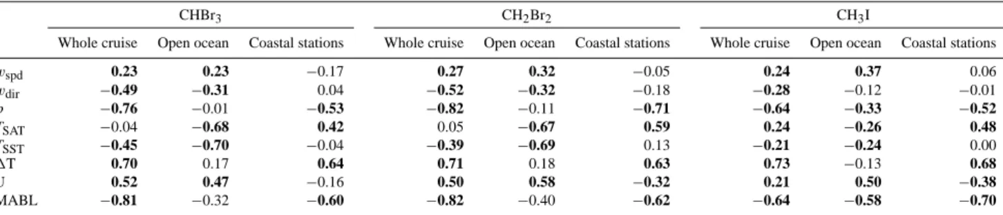
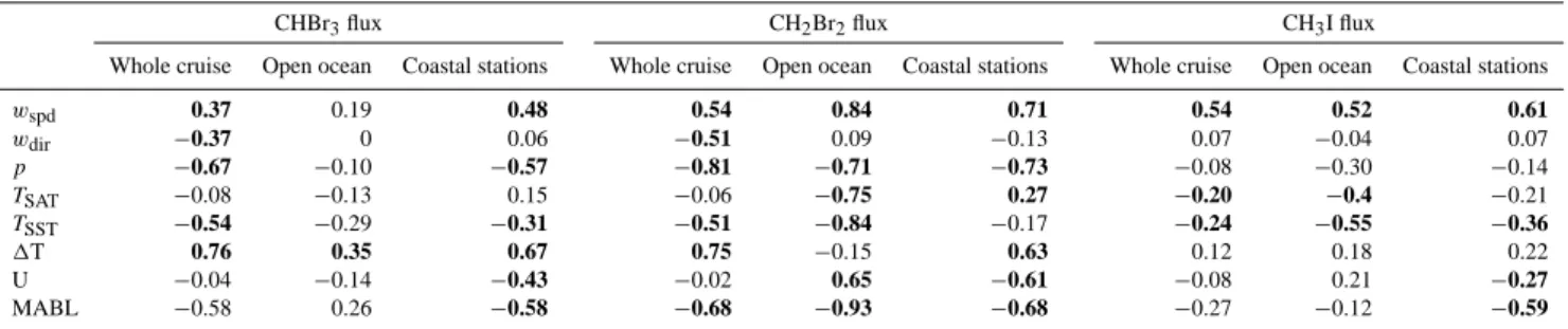
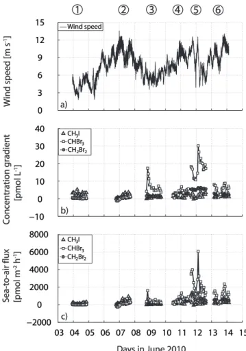
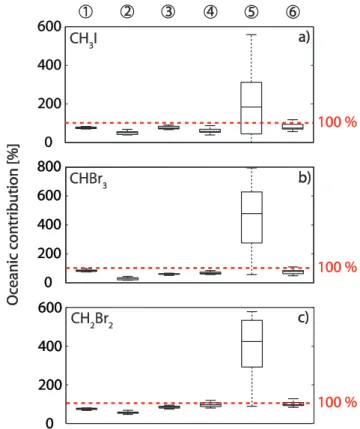
Abstract. During the DRIVE (Diurnal and Regional Vari- ability of Halogen Emissions) ship campaign we investi- gated the variability of the halogenated very short-lived substances (VSLS) bromoform (CHBr₃), dibromomethane (CH₂Br₂) and methyl iodide (CH₃I) in the marine atmo- spheric boundary layer in the eastern tropical and subtropi- cal North Atlantic Ocean during May/June 2010. The highest VSLS mixing ratios were found near the Mauritanian coast and close to Lisbon (Portugal). With backward trajectories we identified predominantly air masses from the open North Atlantic with some coastal influence in the Mauritanian up- welling area, due to the prevailing NW winds. The maxi- mum VSLS mixing ratios above the Mauritanian upwelling were 8.92 ppt for bromoform, 3.14 ppt for dibromomethane and 3.29 ppt for methyl iodide, with an observed maximum range of the daily mean up to 50 % for bromoform, 26 % for dibromomethane and 56 % for methyl iodide. The influence of various meteorological parameters – such as wind, sur- face air pressure, surface air and surface water temperature, humidity and marine atmospheric boundary layer (MABL) height – on VSLS concentrations and fluxes was investigated.

The strongest relationship was found between the MABL height and bromoform, dibromomethane and methyl iodide abundances. Lowest MABL heights above the Mauritanian upwelling area coincide with highest VSLS mixing ratios and vice versa above the open ocean. Significant high anti- correlations confirm this relationship for the whole cruise.

We conclude that especially above oceanic upwelling sys- tems, in addition to sea–air fluxes, MABL height variations can influence atmospheric VSLS mixing ratios, occasionally

leading to elevated atmospheric abundances. This may add to the postulated missing VSLS sources in the Mauritanian upwelling region (Quack et al., 2007).

1 Introduction

Natural halogenated very short-lived substances (VSLS) contribute significantly to the halogen content of the tropo- sphere and lower stratosphere (WMO, 2011). On-going envi- ronmental changes such as increases in seawater temperature and nutrient supply, as well as decreasing pH, are expected to influence VSLS production in the ocean. Thus, the oceanic emissions of VSLS might change in the future and, in con- nection with an altering efficiency of the atmospheric upward transport, might lead to significant future changes of the halo- gen budget of the troposphere/lower stratosphere (Kloster et al., 2007; Pyle et al., 2007; Dessens et al., 2009; Schmit- tner et al., 2008; Montzka and Reimann, 2011), as well as changes to the tropospheric oxidation capacity (Hossaini et al., 2012). Within the group of brominated VSLS, bromo- form (CHBr₃) and dibromomethane (CH₂Br₂) are the largest natural sources for bromine in the troposphere and strato- sphere. In combination with iodine compounds (i.e. methyl iodide, CH₃I), they can alter tropospheric oxidation pro- cesses, including ozone depletion (Read et al., 2008). The VSLS have comparably short tropospheric lifetimes (days to months); however, they can be rapidly transported by deep convection, especially in the tropics, to the upper troposphere and lower stratosphere and contribute to ozone depletion Published by Copernicus Publications on behalf of the European Geosciences Union.