M ARINE ISOPRENE - F ORMATION ,
EMISSIONS AND THEIR IMPACT ON THE ATMOSPHERIC CHEMISTRY
Dissertation
zur Erlangung des Doktorgrades
der Mathematisch-Naturwissenschaftlichen Fakultät der Christian-Albrechts-Universität zu Kiel
vorgelegt von D
ENNISB
OOGEKiel, 2017
M ARINE ISOPRENE - F ORMATION ,
EMISSIONS AND THEIR IMPACT ON THE ATMOSPHERIC CHEMISTRY
Dissertation
zur Erlangung des Doktorgrades
der Mathematisch-Naturwissenschaftlichen Fakultät der Christian-Albrechts-Universität
zu Kiel
vorgelegt von D
ENNISB
OOGEKiel, 2017
Erste Gutachterin: Prof. Dr. Christa A. Marandino Zweiter Gutachter: Prof. Dr. Hermann W. Bange Tag der mündlichen Prüfung: 23.01.2018
Zum Druck genehmigt: 23.01.2018
gez. Prof. Dr. Natascha Oppelt, Dekanin
Eidesstattliche Erklärung
Hiermit erkläre ich, Dennis Booge, dass ich diese Doktorarbeit, abgesehen durch die Beratung meiner Betreuerin, selbstständig verfasst, sowie alle wörtlichen und inhaltlichen Zitate als solche gekennzeichnet habe.
Die Arbeit wurde unter Einhaltung der Regeln guter wissen- schaftlicher Praxis der Deutschen Forschungsgemeinschaft ver- fasst.
Sie hat weder ganz, noch in Teilen, einer anderen Stelle im Rahmen eines Prüfungsverfahrens vorgelegen, ist nicht veröf- fentlicht und auch nicht zur Veröffentlichung eingereicht.
Kiel, Dezember 2017
gez. Dennis Booge
|III
A BSTRACT
Volatile organic compounds (VOCs) play an important role in influencing the oxida- tive capacity of the atmosphere. On a global scale, emissions of biogenic VOCs are dom- inating anthropogenic emissions by one order of magnitude. Isoprene, the most im- portant biogenic VOC, has received increased attention in recent years as biogenic emis- sions of isoprene are the main contributor for secondary organic aerosols (SOA) for- mation. SOA in the atmosphere influence the radiative balance through scattering or absorption of solar radiation and, therefore, have a direct impact on the climate of our Earth’s system. Although terrestrial isoprene emissions are quite well quantified, the strength of global marine isoprene emissions is highly debated, as only a few field meas- urements in the world oceans have been carried out to date. The knowledge about the spatial and seasonal distribution of isoprene, as well as its production and consumption processes in the surface ocean, is still lacking and is crucial to quantify marine isoprene emissions.
The main goal of this work was to increase the global dataset of marine isoprene measurements and provide a better understanding of the biogeochemical cycling in the surface ocean. This improved understanding was used to calculate the global surface isoprene distribution and the isoprene emission to the atmosphere in order to estimate the influence of marine isoprene on the Earth’s atmosphere and climate.
In the first study, isoprene measurements from three different ocean basins were used to improve model simulations of global marine isoprene distributions. Remotely sensed monthly mean satellite data of chlorophyll a (chl-a), sea surface temperature, wind speed, and mixed layer depth were used in a steady-state model to estimate monthly mean global isoprene distributions. Compared to in-field isoprene data, the model under- estimated the actual isoprene concentration by a factor of 19±12. The main improvement was achieved by replacing a single isoprene production rate by chl-a normalized iso- prene production rates from different phytoplankton functional types. However, the im- proved model still could not sufficiently reproduce the distribution pattern and underes- timated the measured concentrations by a factor of two suggesting at least one missing source or possibly other factors influencing surface ocean isoprene distributions. Global marine isoprene emissions were calculated (0.21 Tg C yr-1), increasing earlier emission estimates by a factor of two. However, the calculated emissions had to be 10-20 times higher to account for measured atmospheric isoprene concentrations.
IV|
The goal of the second study was to better understand isoprene sources and sink pro- cesses of isoprene in the surface ocean. Isoprene and related field measurements were carried out in the oligotrophic Indian Ocean as well as in the East Pacific Ocean, in the coastal upwelling region off to Peru. The results of these two contrasting regions demon- strated that isoprene production is mainly influenced by light, ocean temperature, and salinity. Additionally, nutrient availability played a role in the strength of isoprene pro- duction by different phytoplankton types. For the first time, in-field isoprene production rates for different phytoplankton functional types under varying biogeochemical and physical conditions were calculated. By implementing these newly derived production rates into the improved model of the first study, the results indicated that an additional sink process was needed, which was attributed to heterotrophic bacterial respiration.
The results of different global marine isoprene emission estimates were used in the third study to estimate the influence of marine isoprene derived SOA (iSOA) on total atmospheric iSOA concentration. As a result of the first study three different monthly mean emission inventories were used and implemented into a global chemistry climate model (ECHAM-HAMMOZ). A novel framework within ECHAM-HAMMOZ connected the semi-explicit isoprene oxidation chemistry with an explicit treatment of aerosol trac- ers. The results showed that marine iSOA concentrations are very low (contribution:
<1%) compared to total SOA concentrations on a global scale, but are important on re- gional and seasonal scales, as the atmosphere over remote ocean parts was significantly influenced by marine-derived iSOA. Although the annual mean direct radiative effect of marine-derived iSOA in different ocean regions was <0.2 W m-2, the contribution to the total aerosol direct radiative effect on regional and seasonal scales was calculated to be up to 43% (boreal summer, North Atlantic region). However, the effect of marine-derived iSOA on the radiative balance seemed to be weakened due to the formation of larger aerosol particles compared to smaller particle formation over land. The different size distribution might indicate that marine-derived iSOA contributes to the growth of al- ready existing particles instead of contributing to their initial formation.
Despite the low marine-derived iSOA concentrations on a global scale, this thesis il- lustrates that marine isoprene emissions significantly influence the atmospheric chemis- try and the radiative balance in the open ocean regions. In these regions the terrestrial influence is only of minor importance or even absent which strengthens the influence of local marine sources of isoprene on the atmospheric chemistry over the ocean. There- fore, a better understanding of production and consumption of isoprene helps to deter- mine missing sources and sinks influencing surface ocean isoprene distributions to final- ly quantify marine isoprene emissions and their atmospheric impact. The results show that isoprene emission estimates have to be incorporated into atmospheric chemistry climate models in order to predict SOA concentrations and their influence in a changing climate.
|V
Z USAMMENFASSUNG
Flüchtige organische Verbindungen (VOCs: volatile organic compounds) haben einen großen Einfluss auf die oxidative Kapazität der Atmosphäre. Weltweit gesehen sind die Emissionen biogener VOCs um eine Größenordnung stärker als menschengemachte Emissionen. Isopren, als wichtigster Vertreter der biogenen VOCs, wurde in den letzten Jahren zunehmende Aufmerksamkeit zuteil, da es als wichtiger Vorläuferstoff für die Bildung von sekundären organischen Aerosolen (SOA: seconary organic aerosols) ver- antwortlich ist. In der Atmosphäre beeinflusst SOA durch Streuung und Absorption von Sonnenstrahlung die Strahlungsbilanz der Erde und hat somit einen direkten Einfluss auf das Klima. Im Gegensatz zu terrestrischen Emissionen von Isopren ist die Stärke von ozeanischen Emissionen immer noch nicht ermittelt, da bis heute nur wenige Messungen von Isopren in den weltweiten Ozeanen durchgeführt wurden. Sowohl die räumliche und saisonale Verteilung als auch die Bildungs- und Abbauprozesse von Isopren im Oberflä- chenozean sind noch immer nicht ausreichend erforscht. Ein besseres Verständnis dieser Prozesse ist jedoch wichtig um die Stärke mariner Emissionen von Isopren zu quantifi- zieren.
Ziel dieser Arbeit war es Messungen von Isopren im Ozean durchzuführen und die Prozesse sowohl zur Bildung als auch zum Abbau von Isopren im Oberflächenozean zu untersuchen. Die hieraus gewonnenen Erkenntnisse wurden genutzt, um sowohl die globale Konzentrationsverteilung von Isopren im Oberflächenozean als auch die resultie- renden Emissionen in die Atmosphäre zu berechnen, und um somit schlussendlich den globalen Einfluss von ozeanischem Isopren auf das Klima der Erde abschätzen zu kön- nen.
In der ersten Studie wurden Messungen von Isopren in drei verschiedenen Ozeanen genutzt, um die Modellsimulation der globalen Konzentrationsverteilung von Isopren im Oberflächenozean zu verbessern. Mithilfe monatlich gemittelter Satellitendaten von Chlorophyll a (chl-a), der Wassertemperatur, der Windstärke, sowie der Durchmi- schungstiefe wurden globale Konzentrationsverteilungen von Isopren im Oberflä- chenozean berechnet. Im Vergleich zu den Messungen unterschätzte das Modell die Oberflächenkonzentration von Isopren um den Faktor 19±12. Das Modell wurde durch den Einsatz von verschiedenen, je nach Phytoplanktonart abhängigen, chl-a normalisier- ten Isoprenproduktionsraten erheblich verbessert. Jedoch konnte das verbesserte Modell die Konzentrationsverteilung immer noch nicht vollständig wiedergeben. Außerdem
VI|
waren die Konzentrationsvorhersagen im Vergleich zu den Messungen immer noch um das zweifache zu gering. Dies weist auf wenigstens einen oder mehrere nicht berücksich- tigte Prozesse von Isopren im Oberflächenozean hin. Die mit dem neuen Modell berech- neten globalen Isoprenemissionen (0,21 Tg C yr-1) waren doppelt so hoch wie frühere Berechnungen, allerdings um das 10-20 fache zu niedrig, um die gemessenen atmosphä- rischen Isoprenkonzentrationen zu erklären.
Das Ziel der zweiten Studie war es die Produktions- und Abbauprozesse von Isopren im Oberflächenozean zu untersuchen. Dafür wurden Messungen von Isopren und weite- ren Parametern sowohl im nährstoffarmen indischen Ozean als auch im Ostpazifik, im nährstoffreichen Auftriebsgebiet vor Peru, durchgeführt. Die Ergebnisse aus den beiden unterschiedlichen Regionen zeigten, dass die Produktion von Isopren hauptsächlich durch Licht, Wassertemperatur und Salzgehalt beeinflusst wird. Zusätzlich spielte die Verfügbarkeit von Nährstoffen bei einigen Phytoplanktonarten eine Rolle. Zum ersten Mal überhaupt wurden Produktionsraten von Isopren unter verschiedenen biochemi- schen und physikalischen Bedingungen im Ozean berechnet. Diese neu berechneten Produktionsraten wurden in das Modell der ersten Studie implementiert. Die Ergebnisse des aktualisierten Modells zeigten, dass ein zusätzlicher Abbauprozess von Isopren, mög- licherweise bakterielle Respiration, benötigt wird, um die gemessenenen Isoprenkon- zentrationen im Oberflächenozean zu erklären.
Die unterschiedlichen globalen Emissionsabschätzungen von ozeanischem Isopren aus der ersten Studie wurden in der dritten Studie genutzt, um den Einfluss des aus ma- rinem Isopren gebildeten SOA (iSOA) auf die totale atmosphärische iSOA Konzentration abzuschätzen. Dazu wurden drei verschiedene marine Isoprenemissionsszenarien in ein globales, chemisches Klimamodell (ECHAM-HAMMOZ) implementiert. Ein neuer Be- standteil in ECHAM-HAMMOZ verband dabei die semi-explizite Oxidation von Isopren mit einer expliziten Betrachtung von Aerosoltracern. Die Ergebnisse zeigten, dass die marinen iSOA Konzentrationen auf globaler Ebene im Vergleich zu den totalen SOA Konzentrationen sehr gering waren (Anteil: <1%). Jedoch hatten die marinen iSOA Kon- zentrationen über dem offenen Ozean einen signifikanten Einfluss auf regionaler und saisonaler Skala. Der direkte Effekt auf die Strahlungsbilanz über verschiedenen Ozean- regionen war im jährlichen Mittel kleiner 0,2 W m-2. Allerdings war der Anteil am tota- len aerosolinduzierten direkten Effekt auf die Strahlungsbilanz je nach Jahreszeit und Region bis zu 43% (Sommer, Nordatlantik). Der Einfluss von marinem iSOA auf den direkten Strahlungseffekt wird jedoch dadurch geschwächt, dass es bei der Bildung von marinem iSOA zur Bildung von größeren Partikeln kommt als im Vergleich zur Bildung von iSOA über Land. Die unterschiedliche Größenverteilung legt den Verdacht nahe, dass marines iSOA zum Wachstum bereits existierender Partikel und nicht zur deren intitialen Bildung beiträgt.
Auch wenn die marinen iSOA Konzentrationen auf globaler Ebene gering erscheinen, zeigt diese Arbeit, dass marine Emissionen von Isopren die Chemie in der Atmosphäre und die Strahlungsbilanz über dem offenen Ozean signifikant beeinflussen. In diesen Regionen ist der Einfluss terrestrisch gebildeten Isoprens kaum noch vorhanden, was den Einfluss lokaler Ozeanquellen von Isopren auf die Chemie in der Atmosphäre über dem Ozean verstärkt. Dies zeigt, dass ein besseres Verständnis der Produktions- und
|VII Abbauprozesse von Isopren hilft, um die noch fehlenden Quellen und Senken im Ober- flächenozean zu bestimmen. Die gewonnen Erkenntnisse helfen weiter die globale Kon- zentrationsverteilung von Isopren im Oberflächenozean zu berechnen, um so letztendlich den Einfluss von marinen Isoprenemissionen auf die Chemie in der Atmosphäre zu be- stimmen. Die Ergebnisse dieser Arbeit zeigen, dass die Emissionsabschätzungen von marinem Isopren in globale, atmosphärische Klimamodelle integriert werden müssen, um so die SOA Konzentration und deren Einfluss in einem sich verändernden Klima abschätzen zu können.
VIII|
|IX
A CKNOWLEDGEMENTS
Zuallererst bedanke ich mich bei Prof. Dr. Christa Marandino nicht nur für die Mög- lichkeit unter ihrer Aufsicht ein spannendes Thema zu bearbeiten, sondern auch für die wissenschaftliche Unterstützung und das in mich gesetzte Vertrauen bei der Anfertigung dieser Arbeit.
Zudem danke ich den beiden weiteren Mitgliedern meines ISOS-Komitees Dr. Birgit Quack und Prof. Dr. Hermann Bange für ihren wissenschaftlichen Beitrag bei den halb- jährlichen Komitee-Treffen. Dr. Birgit Quack danke ich zusätzlich für ihre kritische Be- trachtungsweise bei der Anfertigung dieser Arbeit.
Den Mitarbeitern und Kollegen sei für die tolle Zeit in den letzten Jahren in der Ab- teilung FB2-CH gedankt. Zusammen haben wir den Chemiker-Cup endlich wieder in die Meereschemie geholt! Spezieller Dank gilt natürlich allen Mitgliedern der AG Marandi- no für das tolle Arbeitsklima und die Hilfe, wann immer sie benötigt wurde.
Bedanken möchte ich mich bei allen Menschen, die mir eine unvergessliche Zeit wäh- rend der beiden Forschungsfahrten mit der FS Sonne bereitet haben. Besonders seien hier natürlich die „Freunde der Sonne“ genannt – „Danke“ für die lange und intensive, aber kurzweilige Arbeitszeit im „Partylabor“ an Bord, aber auch für die lustige und ent- spannte Zeit im Urlaub vor und nach den Forschungsfahrten. Im Speziellen, vielen Dank an das Golden Toyota Corolla Racing Team I: Sinikka und Alex für die „Führungsarbeit“
in Südafrika.
Ein großes Dankeschön an Anna und Alex aus meinem Büro aka „Oval Office“ für die vielen (wohl oder übel) gemeinsam verbrachten, produktiven aber auch lustigen Stunden/Tage/Wochen/Jahre. „Danke“ an Alex für seine immerwährende Geduld bei meinen Fragen zu Matlab.
Vielen Dank an meine Freunde, für die vielen tollen Stunden und Erlebnisse auch au- ßerhalb des Büros (Skatrunde, Spieleabende, BVB-Heimspielbesuche, Urlaube, etc…).
Mein größter Dank gilt meinen Eltern, deren Unterstützung und Rückhalt ich mir immer sicher sein konnte und kann. „Danke“ an Alina und Franzi, dass ihr euch bei der Suche nach Fehlern erfolgreich durch diese Arbeit gekämpft habt und ein zusätzliches großes „Dankeschön“ an dich, Franzi, dass du mir, gerade in der Endphase der Arbeit, immer den Rücken freigehalten hast.
X|
Diese Arbeit wurde im Rahmen von Prof. Dr. Christa Marandinos Helmholtz Young Investigators Group TRASE-EC und des Projektes SO-TRASE (FKZ 03F0782A), unter- stützt durch das Bundesministerium für Bildung und Forschung (BMBF), erstellt.
|XI
L IST OF F IGURES
Figure 1.1: Different components of the climate system showing their radiative forcing (a)
and mean zonal proportion of organic aerosol sources (b). ... 1
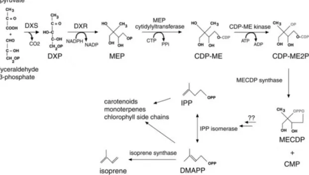
Figure 1.2: The MEP pathway. ... 3
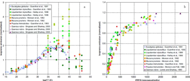
Figure 1.3: Response of isoprene emission to temperature (a) and light (b) ... 4
Figure 1.4: Modeled spatial distribution of monthly mean isoprene emissions ... 4
Figure 1.5: Depth profiles of isoprene (left), chl-a (middle), and different PFTs (right) ... 7
Figure 1.6: Modeled isoprene production and loss rates ... 8
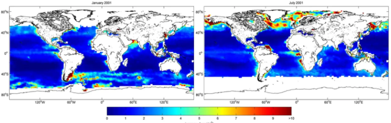
Figure 1.7: Modeled spatial distribution of monthly mean marine isoprene concentrations .... 9
Figure 1.8: Conceptual two-film model (a) and different relationships of the transfer velocity (k) and wind speed (b)... 10
Figure 1.9: Time series of isoprene and methyl vinyl ketone+methacrolein mixing ratios (a), their correlation (b) and light dependent isoprene mixing ratio (c). ... 11
Figure 1.10: Mechanistic overview of the O3 initiated reaction pathways of isoprene ... 13
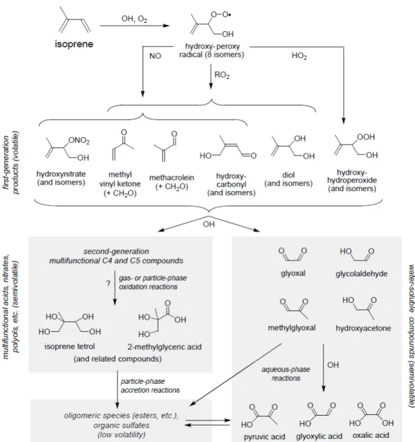
Figure 1.11: Simplified overview of OH initiated pathway of isoprene oxidation leading to SOA (e.g. isoprene tetrol, 2-methylglyceric acid) ... 14
Figure 3.1: System set-up onboard R/V Sonne. ... 31
Figure 3.2: Isoprene recovery percentages of different purge times (a) and a schematic of a sample being purged (b). ... 32
Figure 3.3: Chromatogram of a seawater sample ... 35
Figure 3.4: Schematic of the electron ionization chamber (a) and mass spectrum of isoprene (b). ... 36
Figure 3.5: Schematic of a quadrupole mass filter modified from HÜBSCHMANN (2009) and schematic of an electron multiplier modified from SCHRÖDER (1991). ... 37
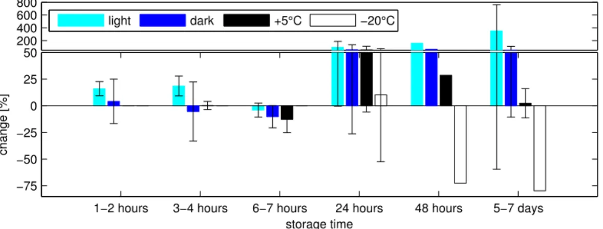
Figure 3.6: Isoprene storage experiment. Mean change in percent of concentration (± standard deviation) under different conditions ... 39
Figure 3.7: Example of a five point calibration using a liquid standard solution. ... 40
Figure 3.8: Sensitivity drift of the system during ASTRA-OMZ cruise 2015. ... 41
XII|
Figure 3.9: Example for calculated m/z=68 calibration peak areas for 1 µL, 10 µL, and 50 µL
standard addition. ... 42
Figure 3.10: Simplified overview of oxidation pathways of isoprene in HAMMOZ ... 46
Figure 4.1: Cruise tracks ... 57
Figure 4.2: Comparison of observed (black) and modeled seawater isoprene concentrations ... 59
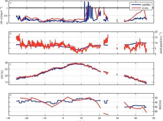
Figure 4.3: Satellite and in situ data for the ANT-XXV/1 cruise. ... 60
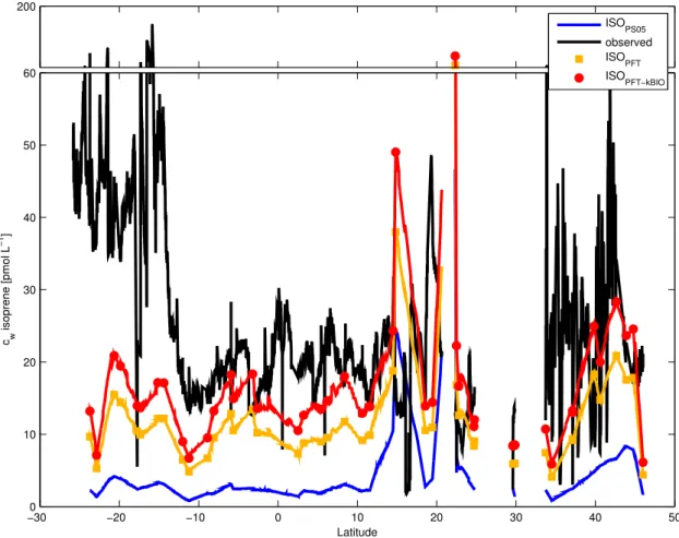
Figure 4.4: Comparison of in situ measured isoprene (black) with model derived isoprene concentrations ... 61
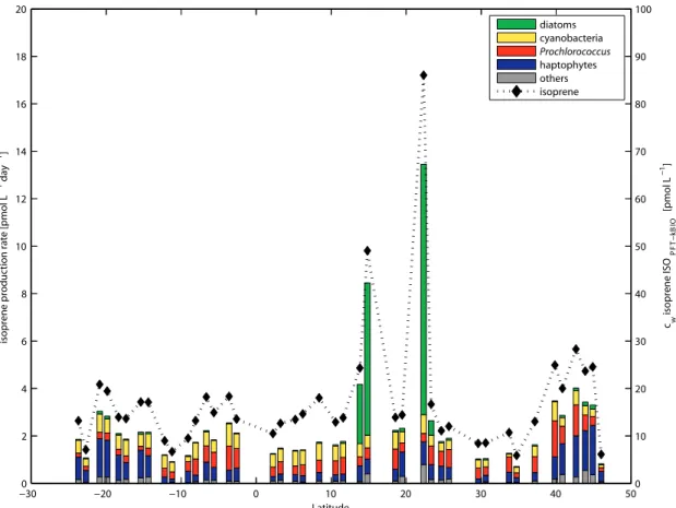
Figure 4.5: Proportion of main PFTs contributing to the total isoprene production rate ... 62
Figure 4.6: Observed isoprene concentration divided by modeled isoprene concentration ... 66
Figure 4.7: Global marine isoprene fluxes in nmol m-2 day-1 for 2014. ... 67
Figure 4.8: 1-day mean measured (blue) and calculated (red) daytime isoprene mixing ratios ... 69
Figure 5.1: Cruise tracks (black) of ASTRA-OMZ (October 2015, East Pacific Ocean) and SPACES/OASIS (July/August 2014, Indian Ocean) ... 89
Figure 5.2: Schematic overview of the analytical purge-and-trap-system ... 90
Figure 5.3: Mean salinity (black), isoprene concentration (blue), temperature (red), and chl-a concentration (green) in the MLD ... 96
Figure 5.4: Mean normalized depth profiles ... 98
Figure 5.5: Percent differences between (a) Pdirect and Pneed ((Pdirect-Pneed)/Pneed) and (b) Pcalc and Pneed ((Pcalc-Pneed)/Pneed) for the different cruises / cruise regions ... 100
Figure 5.6: Mean values (± standard deviation) for (a) calculated Pchloronew haptophytes (blue line) and global radiation (yellow bars), (b) ocean temperature, (c) salinity and (d) nitrate ... 104
Figure 5.7: Relationship between Pnorm in pmol (µg PFT)-1 day-1 and ocean temperature in °C during SPACES (squares), OASIS (triangles), and ASTRA-OMZ (circles) color-coded by NO3- in µmol L-1 ... 105
Figure 5.8: Different mean loss rate constants ... 107
Figure 5.9: Relationship between isoprene concentration [pmol L-1] and total bacteria counts [mL-1] ... 108
Figure 5.10: Mean values (± standard deviation) for (a) kconsumption [day-1], (b) total bacteria counts [mL-1] and (c) AOU [µmol L-1] ... 109
Figure 6.1: Annual mean global marine isoprene emissions for 2012. ... 129
Figure 6.2: Seasonal mean atmospheric isoprene concentrations above the ocean for 2012. 131 Figure 6.3: Seasonal mean iSOA concentrations for 2012. ... 133
Figure 6.4: Impact of oceanic isoprene emissions on iSOA formation and iSOA burden. ... 136
|XIII Figure 6.5: Annual mean and seasonal trend of marine-derived and terrestrially derived iSOA ... 137 Figure 6.6: Direct radiative effect of marine-derived iSOA in four different ocean regions. . 139 Figure 6.7: Size distributions of iSOA in different regions. ... 141 Figure 7.1: Modeled surface ocean isoprene concentrations. ... 148 Figure 7.2: Contribution of marine-derived iSOA to total iSOA in %. ... 150 Figure 7.3: Schematic diagram of main isoprene pathways and processes in the marine and atmospheric environment including corresponding potential feedbacks in a warming climate. ... 153 Figure 7.4: Projected change in global abundance of Prochlorococcus (A) and Synechococcus (B) for 2100 ... 154
XIV|
|XV
L IST OF T ABLES
Table 1.1: Literature review of published field studies of marine isoprene concentrations ... 5
Table 3.1: Properties and retention times of isoprene and other gases analyzed with the measurement set-up. ... 33
Table 3.2: Temperature program of the used GC-method. ... 34
Table 3.3: Four low volatility organic compound oxidation products contributing to isoprene derived secondary organic compounds. ... 46
Table 4.1: List of parameters used in each model. ... 56
Table 4.2: Chlorophyll-normalized isoprene production rates (Pchloro)... 64
Table 5.1: Factors of different regression equations from different studies ... 88
Table 5.2: Emission factor (EF) of each PFT ... 94
Table 5.3: Calculated chl-a normalized isoprene production rates ... 102
Table 6.1: Global SOA modeling studies. ... 126
Table 6.2: Comparison of global oceanic isoprene emissions ... 127
Table 6.3: Annual global isoprene emissions and iSOA formation ... 134
XVI|
|XVII
M ANUSCRIPT OVERVIEW
This thesis is based on the following manuscripts:
1. Dennis Booge, Christa A. Marandino, Cathleen Schlundt, Paul I. Palmer, Mi- chael Schlundt, Elliot L. Atlas, Astrid Bracher, Eric S. Saltzman, Douglas W. R.
Wallace: Can simple models predict large scale surface ocean isoprene concentrations?, published in: Atmos. Chem. Phys., 16, 11807–11821, 2016, doi:10.5194/acp-16-11807-2016.
Author contribution: Dennis Booge designed the study together with Christa A.
Marandino, performed the data analysis and wrote the manuscript. Christa A.
Marandino measured oceanic isoprene on board together with Cathleen Schlundt and wrote parts of the manuscript. Astrid Bracher analyzed the pigment data and Elliot L. Atlas measured isoprene concentrations in the air. Paul I. Palmer helped to validate model calculations and Michael Schlundt calculated mixed layer depths of the cruises. All authors reviewed the manuscript.
2. Dennis Booge, Cathleen Schlundt, Astrid Bracher, Sonja Endres, Birthe Zänck- er, Christa A. Marandino: Marine isoprene production and consumption in the mixed layer of the surface ocean – A field study over 2 oceanic regions, accepted for publication in Biogeosciences, doi:10.5194/bg-2017-257.
Author contribution: Dennis Booge performed the isoprene measurements on board, analyzed the isoprene data, and wrote the manuscript. Cathleen Schlundt and Christa A. Marandino performed the isoprene measurements on board.
Astrid Bracher analyzed the pigment and radiation data. Sonja Endres and Birthe Zäncker performed the HPLC measurements and analyzed the bacteria data. All authors reviewed the manuscript.
XVIII|
3. Dennis Booge, Scarlet Stadtler, Christa A. Marandino: The influence of ma- rine isoprene emissions on secondary organic aerosol concentration over the remote ocean, manuscript in preparation.
Author contribution: Dennis Booge designed the study together with Christa A.
Marandino, performed the isoprene data analysis and wrote the manuscript with contribution from all authors. Scarlet Stadtler performed the secondary organic aerosol model calculations.
In addition, I contributed to the following manuscripts:
4. Lennartz, S. T., Marandino, C. A., von Hobe, M., Cortes, P., Quack, B., Simo, R., Booge, D., Pozzer, A., Steinhoff, T., Arevalo-Martinez, D. L., Kloss, C., Bracher, A., Röttgers, R., Atlas, E., and Krüger, K.: Direct oceanic emissions unlikely to account for the missing source of atmospheric carbonyl sulfide, published in:
Atmos. Chem. Phys., 17, 385-402, 2017, doi:10.5194/acp-17-385-2017, 2017.
5. Alex Zavarsky, Dennis Booge, Alina Fiehn, Kirstin Krüger, Elliot Atlas and Christa Marandino: The influence of air-sea fluxes on atmospheric aerosols dur- ing the summer monsoon over the tropical Indian Ocean, published in Geophys.
Res. Lett., 45, doi:10.1002/2017GL076410, 2017.
6. Lennartz, S. T., Marandino, C. A., von Hobe, M., Fischer, T., Bittig, H., Booge, D., Goncalves Araujo, R., Ksionzek, K., Koch, B. P., Bracher, A., Röttgers, R., Quack, B.: Production and Consumption processes of OCS and CS2 in the Eastern Tropical South Pacific, manuscript in preparation for J. Geophys. Res .
|XIX
C ONTENTS
ABSTRACT III
ZUSAMMENFASSUNG V
ACKNOWLEDGEMENTS IX
LIST OF FIGURES XI
LIST OF TABLES XV
MANUSCRIPT OVERVIEW XVII
CONTENTS XIX
1 INTRODUCTION 1
1.1 Terrestrial isoprene ... 2 1.1.1 Production ... 2 1.1.2 Spatial distribution ... 4 1.2 Marine isoprene ... 5 1.2.1 Sources ... 6 1.2.2 Sinks. ... 7 1.2.3 Spatial distribution ... 8 1.3 Air-sea gas exchange ... 9 1.4 Isoprene in the atmosphere ...11 1.4.1 Atmospheric distribution ...11 1.4.2 Atmospheric reactions ...12 1.4.3 SOA formation ...13 1.5 Climate feedbacks ...15
2 THESIS OUTLINE 29
XX|
3 METHODS 31
3.1 Analytical quantification of isoprene ... 31 3.1.1 Purge & Trap technique ... 31 3.1.2 Gas chromatography ... 34 3.1.3 Mass spectrometry ... 35 3.2 General sampling and analytical procedure ... 37 3.3 Storage tests ... 38 3.4 Data analysis ... 39 3.4.1 Calibrations ... 39 3.4.2 Sensitivity drift ... 41 3.4.3 Error analysis ... 43 3.5 The chemistry climate model ECHAM-HAMMOZ ... 45 3.5.1 Modification for isoprene derived SOA formation ... 45
4 MODELING MARINE ISOPRENE CONCENTRATIONS 51
4.1 Introduction ... 52 4.2 Methods ... 53 4.2.1 Model description... 53 4.2.2 Cruise tracks ... 56 4.2.3 Isoprene measurements ... 57 4.3 Results and discussion ... 58 4.3.1 Comparison of modeled and in situ measured isoprene data ... 58 4.3.2 Modeling isoprene production using PFTs and revised kBIOL ... 61 4.3.3 Verification of the ISOPFT-kBIOL model using data from the Indian and
eastern Pacific Oceans ... 66 4.4 Global oceanic isoprene emissions and implications for marine aerosol
formation ... 67 4.5 Conclusions ... 70 4.6 Data availability ... 71 4.7 Acknowledgements ... 71 4.8 Supplementary material ... 71
5 PRODUCTION AND CONSUMPTION OF ISOPRENE 85
5.1 Introduction ... 86 5.2 Methods ... 89
|XXI 5.2.1 Sampling sites ...89 5.2.2 Isoprene measurements ...90 5.2.3 Nutrient measurements ...91 5.2.4 Bacteria measurements ...91 5.2.5 Phytoplankton functional types from marker pigment
measurements ...91 5.2.6 Photosynthetic available radiation within the water column
measurements ...92 5.2.7 Calculation of isoprene production ...93 5.3 Results and discussion ...95 5.3.1 Cruise settings ...95 5.3.2 Isoprene distribution in the mixed layer ...97 5.3.3 Modeling chl-a normalized isoprene production rates...99 5.3.4 Drivers of isoprene production ... 103 5.3.5 Loss processes ... 106 5.4 Conclusions ... 110 5.5 Data availability ... 111 5.6 Acknowledgements ... 111 5.7 Supplementary material ... 112 6 INFLUENCE OF MARINE ISOPRENE EMISSIONS ON SOA FORMATION 125 6.1 Introduction ... 125 6.1.1 Global isoprene derived SOA ... 125 6.1.2 Marine isoprene emissions ... 126 6.2 Methods ... 128 6.2.1 Model description ... 128 6.2.2 Marine isoprene emissions ... 128 6.3 Results and discussion ... 130 6.3.1 Atmospheric isoprene distribution ... 130 6.3.2 Global iSOA distribution... 132 6.3.3 Regional and seasonal impacts ... 135 6.3.4 Direct radiative effect ... 138
7 CONCLUSION AND OUTLOOK 147
CURRICULUM VITAE 159
XXII|
|1
1 I NTRODUCTION
Aerosols influence the radiative balance of our Earth’s system directly through ab- sorption and scattering of solar radiation, or indirectly, through formation of cloud con- densation nuclei (IPCC, 2013). They have a negative radiative forcing potential and, therefore, counteract the warming potential of greenhouse gases (Figure 1.1a). Aerosols are either emitted directly (primary aerosols) from natural (e.g. volcanic eruption, sea spray) or anthropogenic sources (e.g. combustion process) or are formed in the atmos- phere (secondary aerosols) by gas-particle processes through heterogeneous or multi- phase chemical reactions (e.g. sulfates, nitrates, organic compounds). Organic aerosol (OA) represents the dominant component of global aerosol (KANAKIDOU et al., 2005) and is divided similarly into primary OA (POA) and secondary OA (SOA). SOA is formed by volatile organic compounds (VOC), which act as precursor gases in the atmosphere (PANDIS et al., 1992). Globally, 90% of SOA is due to biogenic emissions of VOCs (KANAKIDOU et al., 2005). However, in the northern hemisphere, anthropogenic sources are suggested to be equally important (DE GOUW and JIMENEZ, 2009; LIN et al., 2012) (Figure 1.1b).
One of the biogenic VOCs is isoprene (2-methyl-1,3-butadiene), which has received the most attention in recent years concerning its terrestrial importance for SOA for-
Figure 1.1: Different components of the climate system showing their radiative forcing (a) and mean zonal proportion of organic aerosol sources (b). (a) Globally averaged radiative forcing for the period 1750-2011 with uncertainties (5 to 95% confidence range) from IPCC (2013). (b) Estimated zonal mean distribution of different SOA and POA sources as fraction of total organic aerosol from DE GOUW and JIMENEZ (2009). BB: biomass burning. Note: no differentiation of primary and secondary derived marine OA.
a b
2|
mation (CARLTON et al., 2009). Once emitted to the atmosphere, isoprene is highly reac- tive and influences more than SOA formation. Through reaction with OH, isoprene oxi- dation affects the lifetime of the greenhouse gas methane (COLLINS et al., 2002). Addi- tionally, isoprene oxidation products can increase tropospheric ozone levels during high nitrogen oxides (NOx) levels (HOFZUMAHAUS et al., 2009). On the other hand, during low NOx levels, isoprene directly reacts with ozone, decreasing atmospheric ozone levels (ATKINSON and AREY, 2003).
Isoprene has the highest global emission estimate of all biogenic VOCs with flux es- timates of 410 - 600 Tg C yr-1 (ARNETH et al., 2008). Terrestrial emissions from plants are dominant and only a minor amount (~1 Tg C yr-1) is attributed to marine emissions (SHAW et al., 2010 and references therein). The contribution of marine-derived SOA to the total global SOA budget is highly discussed (MESKHIDZE and NENES, 2006). It appears relatively small on a global basis (GANTT et al., 2010) but could be up to 100% over the Southern Ocean (DE GOUW and JIMENEZ, 2009).
Determination and prediction of aerosol production and its radiative forcing poten- tial in models is an important research topic in atmospheric chemistry and climate change research. However, there are large uncertainties in global models trying to esti- mate the current and future influence of aerosols on the radiative balance of the Earth’s system. A part of these uncertainties can be reduced by fully understanding the for- mation of SOA through isoprene oxidation. Particularly, the understanding of the com- position and formation of marine SOA is limited and needs further research to quantify the influence of oceanic isoprene emissions on atmospheric SOA formation. In the fol- lowing sections the current knowledge of the formation of isoprene, its marine and ter- restrial source, and its emissions to the atmosphere will be discussed. Furthermore, an overview of the mechanistic understanding of atmospheric isoprene oxidation to SOA formation will be given.
1.1 Terrestrial isoprene
1.1.1 Production
The emission of isoprene by plants was discovered 60 years ago (SANADZE, 1957) and was firstly quantified using mass spectrometry by SANADZE (1969) and RASMUSSEN
(1970). Isoprene is synthesized in chloroplasts of plants from the precursor dimethylallyl pyrophosphate (DMAPP) using the enzyme isoprene synthase (SILVER and FALL, 1991).
DMAPP is produced by the 2-methylerythritol 4-phosphate (MEP) pathway starting with the reaction of pyruvate and glyceraldehyde 3-phosphate (ROHMER et al., 1993). Fig- ure 1.2 shows the MEP pathway, including the energetic costs. SHARKEY and SINGSAAS
(1995)MILNE et al. (1995)MILNE et al. (1995) To date, it is still unclear if isopentenyl py- rophosphate (IPP) is produced first, which then can be isomerized to DMAPP, or if DMAPP is formed directly. Monoterpenes and carotenoids can also be formed via the
|3 MEP pathway. Plants that do not have the enzyme isoprene synthase are not able to pro- duce and emit isoprene. The MEP pathway costs 6 carbon atoms, 20 adenosine triphos- phates (ATP), and 14 nicotinamide adenine dinucleotide phosphates (NADPH) to pro- duce isoprene. The benefits plants derive from isoprene emissions are highly debated, because some plants do emit isoprene whereas others do not (SHARKEY and YEH, 2001).
The most discussed advantage plants may gain from producing isoprene is thermotoler- ance (Figure 1.3a), which was first observed by SHARKEY and SINGSAAS (1995). This pro- tection against heat stress involves the protection from direct solar radiation resulting in heat or sunflecks (SHARKEY et al., 2008). Leaves at the top of a canopy, which are ex- posed to higher light levels than those at the bottom, emit up to four times more isoprene (HARLEY et al., 1996). The light dependence of isoprene emission in plants is well known and emissions increase with increasing light intensity (Figure 1.3b). Isoprene may also serve as antioxidant because it rapidly reacts with ozone or other reactive oxygen species (STOKES et al., 1998). Atmospheric CO2 levels are also thought to influence isoprene emissions, but there are contradicting results. Some studies suggest that isoprene emis- sions are inhibited at high CO2 levels (TINGEY et al., 1981), whereas other studies suggest that isoprene emissions are enhanced, which may also be plant dependent (SHARKEY et al., 1991).
Figure 1.2: The MEP pathway. CDP-ME, 4-(cytidine 5’-diphospho)-2-C-methyl-D-erythritol; CDP-ME2P, 2-phospho-4-(cytidine 5’-diphospho)-2-C-methyl-D-erythritol; DMAPP, dimethylallyl pyrophosphate;
DXR, deoxyxylulose-5-phosphate reductoisomerase; DXS, deoxyxylulose-5-phosphate synthase; IPP, iso- pentenyl pyrophosphate; MECDP, 2-C-methyl-D-erythritol 2,4-cyclodiphosphate. Modified from SHARKEY and YEH (2001).
4|
1.1.2 Spatial distribution
Figure 1.4 shows monthly mean spatial distributions of terrestrial isoprene emissions using a terrestrial ecosystem emission model (MEGAN, GUENTHER et al., 2012). The global mean annual isoprene emission estimate over the period of 1980-2010 is 594 ± 34 Tg (SINDELAROVA et al., 2014), which is comparable to other global isoprene emission estimates ranging from 410 Tg yr-1 (MÜLLER et al., 2008) to 635 Tg yr-1 (POTTER
et al., 2001). Although the emission estimates differ in various studies, the spatial distri- bution of terrestrial isoprene emissions is similar in each study. Strongest isoprene emis- sions can be seen in tropical and south-tropical regions, driven by high temperatures and incoming solar radiation. Northern and southern tropics account for 88% of total terres- trial isoprene emissions. The strength of isoprene emissions is shifted towards to the southern hemisphere during austral summer (Figure 1.4a) and to the northern hemi- sphere during boreal summer (Figure 1.4b).
Figure 1.3: Response of isoprene emission to temperature (a) and light (b) from PACIFICO et al. (2009).
PPFD: Photosynthetic photon flux density in µmol m-2 s-1, T: temperature in °C.
a b
Figure 1.4: Modeled spatial distribution of monthly mean isoprene emissions in mg m-2 day-1 for (a) Janu- ary and (b) July averaged over the period 1980-2010 from SINDELAROVA et al. (2014).
|5
1.2 Marine isoprene
Evidence for the marine production of isoprene was found for the first time in the early 1990s by BONSANG et al. (1992). They performed isoprene measurements in the atmosphere and in the ocean. Due to the supersaturation in the water they concluded that it has to be produced in the marine environment. Furthermore, they proposed that it is produced biologically because the isoprene concentration was mainly following the fluorescence signal of their measurements when performing vertical profiles. Since then, 15 more studies of field measurements were published in order to quantify isoprene con- centrations in different parts of the ocean (general range: <1 - 200 pmol L-1; references:
Table 1.1). Furthermore, laboratory studies under varying conditions were performed in order to investigate the influence of physical and physiological parameters on the pro- duction and consumption of isoprene in the marine environment. A state-of-the-art overview of processes driving the isoprene production and consumption is given in the following sections.
Table 1.1: Literature review of published field studies of marine isoprene concentrations in pmol L-1.
Reference Region Month Concentration
BONSANG et al. (1992) Pacific Ocean, Mediterranean Sea
April, May/October
3.6 - 98
MILNE et al. (1995) Florida Straits, Gulf Stream
September 9.8 - 51
BROADGATE et al. (1997) Southern Ocean, North Sea
November 0.7 - 90
BAKER et al. (2000) Eastern Atlantic Ocean May 5 - 55 MATSUNAGA et al. (2002) Western North Pacific May <12 - 94 BROADGATE et al. (2004) Mace Head, Ireland September 10 - 21 WINGENTER et al. (2004) Southern Ocean January mean: 1.8 MOORE and WANG (2006) Eastern North Pacific July 2 - 6.5 KURIHARA et al. (2010) Western North Pacific April 4 - 68 KURIHARA et al. (2012) Sagami Bay April - December 4.4 - 10
TRAN et al. (2013) Arctic Ocean July mean: 26 ± 31
KAMEYAMA et al. (2014) Southern (Indian) Ocean January 0.2 - 395
ZINDLER et al. (2014) Eastern Atlantic Ocean November mean: 25.7 ± 14.7 OOKI et al. (2015) Southern Ocean, Indian
Ocean, Northwest Pacific Ocean, Bering Sea, west- ern Arctic Ocean
September - November, November - January, April - September, Octo- ber, September
basin: 1.3 - 121 slope: 1.5 - 165 shelf: 2.7 - 136
6|
Table 1.1: Literature review of published field studies of marine isoprene concentrations in pmol L-1.
Reference Region Month Concentration
LI et al. (2017) East China Sea, South Yellow Sea
July 32 - 174
HACKENBERG et al. (2017) Atlantic Ocean, Arctic Ocean
October/November, March/July
1 - 66
1.2.1 Sources
Biological production. Oceanic isoprene concentrations mainly follow the chloro- phyll a (chl-a) depth profile (BONSANG et al., 1992; HACKENBERG et al., 2017; MILNE et al., 1995; TRAN et al., 2013). Using different monocultures of phytoplankton functional types (PFTs) in laboratory studies, MILNE et al. (1995) could prove that isoprene is produced biologically by phytoplankton. Figure 1.5 shows a typical depth profile of isoprene, which follows the shape of the chl-a profile and the profile of some abundant PFTs.
However, further studies discovered that not every PFT has the same ability to produce isoprene (SHAW et al., 2010 and references therein). Measured chl-a normalized isoprene production rates from monocultures range from 0.36 ± 0.22 µmol (g chl-a)-1 day-1 (species of chlorophytes; BONSANG et al., 2010) up to 32.16 ± 5.76 µmol (g chl-a)-1 day-1 (species of prasinophytes; EXTON et al., 2013). The strength of isoprene emissions is mainly attributed to environmental conditions like light and temperature stress (EXTON
et al., 2013; MESKHIDZE et al., 2015; SHAW et al., 2003) which is similar to terrestrial iso- prene emissions. Generally, isoprene production rates increase with increasing light lev- els and increasing temperature, but also might level off or even decrease at higher light or temperature levels. The influence of light and temperature varies already within one group of phytoplankton (MESKHIDZE et al., 2015; SRIKANTA DANI et al., 2017). These re- sults suggest a similar physiological function of isoprene for phytoplankton in the ocean as for terrestrial plants on land.
Chemical production. An additional source for isoprene could be the reaction of photochemically excited dissolved organic matter and fatty acids in the surface micro- layer (SML) of the ocean. In reactor experiments CIURARU et al. (2015) measured iso- prene in the gas phase immediately after illuminating sea water containing humic acid (acts as dissolved organic matter) and nonanoic acid (surfactant). If a surfactant was not added, no isoprene emission was observed. Surfactant concentration is known to be high in the SML (WURL et al., 2011), therefore a photochemical reaction of organic matter with surfactants could be a hint of non-biological production of isoprene in the marine environment.
continued.
|7
1.2.2 Sinks.
Biological consumption. Very little is known about bacterial degradation of iso- prene in seawater. ACUÑA ALVAREZ et al. (2009) tested some bacteria species and could show that bacterial degradation might take place. Recently, JOHNSTON et al. (2017) iden- tified isoprene degrading bacteria strains in estuarine and marine environments. Howev- er, these studies did not provide any isoprene loss rates and they are thought to be very small compared to the biological production (SHAW et al., 2003).
Chemical degradation. Even less is known about chemical degradation of isoprene in seawater and only assumptions were made to date. PALMER and SHAW (2005) used rates for the reaction with OH in the gas phase and for the reaction with singlet oxygen in chloroform (Figure 1.6). Scaling these rates with the oceanic concentration of each oxidant (OH=10-17 mol L-1, singlet oxygen=10-14 mol L-1 from COOPER et al. (1988)) leads to mean isoprene loss rates <10% of the biological production rates of isoprene (PALMER
and SHAW, 2005).
Air-sea gas exchange. The dominant loss of isoprene in the ocean is thought to be the gas exchange to the atmosphere. The lifetime of isoprene due to air-sea gas exchange is about seven days in the mixed layer of the ocean (PALMER and SHAW, 2005) and the loss rate is highest in the high latitudes during seasons of high wind speeds (Figure 1.6).
Theoretically, air-sea gas exchange can also be a source for oceanic isoprene, but as iso- prene is generally oversaturated in the surface ocean by up to three orders of magnitude (BONSANG et al., 1992; MILNE et al., 1995; WINGENTER et al., 2004), the air-sea gas ex- change is a net loss for marine isoprene. The strength of isoprene emissions to the at-
Figure 1.5: Depth profiles of isoprene (left), chl-a (middle), and different PFTs (right) in the Arctic Ocean during summer 2010 from TRAN et al. (2013).
8|
mosphere depends on the concentration difference between the ocean and the atmos- phere but also on parameters like wind speed and temperature. The concept of air-sea gas exchange and its driving processes are explained in section 1.3.
1.2.3 Spatial distribution
Figure 1.7 shows the modeled monthly mean isoprene concentrations in the surface mixed layer of the ocean. PALMER and SHAW (2005) used chl-a concentrations as a proxy to parameterize surface ocean isoprene concentrations, as isoprene is produced biologi- cally (see section 4.2.1). Therefore, surface ocean isoprene concentrations show a similar distribution pattern as the chl-a concentration distribution in the ocean with very low concentrations in the tropical ocean due to oligotrophic conditions. During boreal sum- mer, open ocean isoprene concentrations increase in the northern hemisphere, with local hotspots of phytoplankton blooms. During austral summer, isoprene concentrations are higher in the southern hemisphere, also with local hotspots of phytoplankton blooms in the open ocean. However, surface ocean isoprene concentrations are lower, compared to the northern hemisphere summer time, because constant high wind speeds are pushing the air-sea gas exchange. Isoprene concentrations are enhanced in coastal regions, main- ly due to regional and seasonal hotspots of biological activity.
Figure 1.6: Modeled isoprene production and loss rates as a function of latitude and season using satellite data from PALMER and SHAW (2005).
|9
1.3 Air-sea gas exchange
The flux across the air-sea-interface is the only source for atmospheric isoprene over the remote ocean, where the influence of terrestrially derived isoprene is negligible. The transfer (F) of a gas is controlled by the transfer velocity (k) and the concentration gradi- ent (∆C) between the water- (Cw) and the air-phase (Ca):
F = k ∆C = k Cw - Ca (1.1)
The physical and chemical properties influence the solubility of each gas in a liquid medium. Therefore the Ostwald coefficient (α) is used to correct for the solubility of each gas:
F = k Cw - α Ca (1.2)
The transfer of a gas at the interface depends on the solubility and is either controlled in the water or in the air-side and is described by the two-film model by LISS and SLATER
(1974). In this conceptual model, shown in Figure 1.8a, the exchange depends on the mo- lecular diffusion at the interface in between the turbulent layer of the air and the water.
The resistance for soluble gases, like water vapor or sulfur dioxide (α ≥ 100), is air-side controlled (red line), whereas for insoluble gases like isoprene (blue line), the resistance is controlled by the aqueous-side diffusive sublayer (WANNINKHOF et al., 2009).
The transfer velocity (k) describes the kinetic force controlling the gas transfer. Many processes influence the transfer velocity and are mainly wind induced, including break- ing waves and bubble entrainment (e.g. ASHER et al., 1996; ZHANG et al., 2006). Surface films (e.g. BROECKER, 1978) or rain (e.g. HO et al., 1997) also affect k. Today, different approaches are carried out in the field in order to determine k. The turbulent flux F above the interface can be directly measured using micrometeorological techniques, like the eddy covariance technique (e.g. MARANDINO et al., 2007; MCGILLIS et al., 2001). Val- ues for k can be directly derived using equation (1.1) when both the F and ∆C are meas- ured simultaneously. Another technique is the so called mass balance technique. The dual tracer method is one of several techniques, where the mass balance of a gas in the water is perturbed by adding a mixture of 3He/SF6-gas to the water (e.g. HO et al., 2006;
Figure 1.7: Modeled spatial distribution of monthly mean marine isoprene concentrations in the surface mixed layer in pmol L-1 for January 2001 (left) and July 2001 (right). Isoprene concentrations were calcu- lated from isoprene emission estimates from PALMER and SHAW (2005).
10|
WANNINKHOF et al., 1993). As these gases are inert, measurements of Cw and Ca over time yield the flux F.
Measurements have shown that wind speed has a dominant effect and, therefore, is a good indicator to describe the gas transfer (e.g. BELL et al., 2013; HO et al., 2011;
WANNINKHOF et al., 2009). Since LISS and MERLIVAT (1986) published the first wind speed based parameterization, different other parameterizations (e.g., quadratic, cubic) were published and are shown in Figure 1.8b. During this work three different wind speed (at 10 m height, U10) based parameterizations were applied to calculate isoprene emissions:
kW92=0.31 U102 660SC-0.5 , WANNINKHOF (1992) (1.3)
kW99=0.0283 U103 660SC-0.5, WANNINKHOF and MCGILLIS (1999) (1.4)
kN00=0.333 U10+0.222 U102 660SC-0.5 , NIGHTINGALE et al. (2000) (1.5) The temperature (T) dependent dimensionless Schmidt number (SC) of isoprene, which is the ratio of the molecular diffusivity of isoprene in seawater and the kinematic viscosity of seawater, is taken from PALMER and SHAW (2005):
SC = 3913.15 - 162.13T + 2.67T2 - 0.012T3 (1.6)
The parameterizations are generally comparable in a wind regime <7 m s-1, but the differences increase significantly at higher wind. Other factors like surface films or bub- ble entrainment are one hypothesis to explain the divergence in parameterizations at higher wind speeds. It is very important to reduce the uncertainties of theses parameteri- zations in the future, especially at high wind speeds. A better assessment of flux esti- mates of climate relevant gases will improve to estimate their influence on the chemistry in the atmosphere today and in a changing climate.
Figure 1.8: Conceptual two-film model (a) and different relationships of the transfer velocity (k) and wind speed (b). (a) Concentration profile of an insoluble gas (blue line) and a soluble gas (red line) from WAN- NINKHOF et al. (2009). (b) Parameterizations and results for k from 3He/SF6 dual tracer experiments de- pendent on the wind speed from HO et al. (2011).
|11
1.4 Isoprene in the atmosphere
1.4.1 Atmospheric distribution
Total global emissions of isoprene range from 410 to 600 Tg C yr-1 (ARNETH et al., 2008). Oceanic emissions of isoprene represent only a minor amount. Depending on model simulations (“bottom-up” or “top-down” approaches) global oceanic emission es- timates range from 0.1 to 11.6 Tg C yr-1 (ARNOLD et al., 2009; GANTT et al., 2009; LUO
and YU, 2010; PALMER and SHAW, 2005). Due to the short lifetime of 1 - 4 hours (SHAW et al., 2010 and references therein), mean daily atmospheric concentrations in the terrestri- al boundary layer are generally <1 ppb but can be up to 11 ppb and 26 ppb during day- time over the central amazon forest and an oil palm plantation, respectively (JARDINE et al., 2016; MISZTAL et al., 2011). Isoprene concentrations in the atmosphere over the re- mote oceans are generally lower than 100 ppt (YOKOUCHI et al., 1999). Concentrations in the marine atmosphere are mainly influenced by light, as shown in Figure 1.9 (LIAKAKOU
et al., 2007). This is due to higher emissions from phytoplankton during
Figure 1.9: Time series of isoprene and methyl vinyl ketone+methacrolein mixing ratios (a), their correla- tion (b) and light dependent isoprene mixing ratio (c). (a) Time series of isoprene and MVK+MACR in ppbv over a palm oil plantation in Malaysian Borneo from MISZTAL et al. (2011). (b) Correlation of iso- prene and its oxidation products MVK+MACR volume mixing ratios (r2=0.80) in the atmosphere over the Southern Indian Austral Ocean from COLOMB et al. (2009). (c) Atmospheric isoprene mixing ratios in ppbv from unpolluted marine air dependent on light intensity (W m-2) from a coastal site on the island of Crete in the East Mediterranean from LIAKAKOU et al. (2007).
12|
daytime, which is similar to emissions from plants. LEWIS et al. (1997) measured a diel cycle of isoprene concentrations in marine influenced atmosphere at a coastal station in Mace Head, Ireland. The diel cycle was similar to the variation in concentration from terrestrial influenced air with the highest concentrations during 12 pm and 2 pm.
The spatial and seasonal distribution in the terrestrial atmosphere is similar to the ter- restrial emission distributions of isoprene (Figure 1.4), as transport of atmospheric iso- prene is of minor importance due to the short lifetime. Generally, the same is true for isoprene in the marine boundary layer. Atmospheric concentrations over the North At- lantic (during boreal winter) and the Southern Ocean (throughout the whole year) are comparatively higher than marine concentrations due to strong winds driving the iso- prene gas exchange from the ocean to the atmosphere.
1.4.2 Atmospheric reactions
Once emitted to the atmosphere isoprene is highly reactive, due to the two double bonds, and influences the oxidative capacity of the atmosphere (CARLTON et al., 2009).
The short lifetime of isoprene is mainly dependent on the atmospheric reactions with hydroxyl radicals (OH), nitrate (NO3), and ozone (O3). The rate constant (at 298 K) for the reaction of isoprene with OH is highest (1.0×10⁻¹¹ cm3 molecule-1 s-1), followed by the reaction with NO3 (6.8×10⁻¹³ cm3 molecule-1 s-1) and O3 (1.3×10⁻¹⁷ cm3 molecule-1 s-1) (ATKINSON et al., 2006). Isoprene directly modulates the O3 concentration (WILLIAMS et al., 2010), but also, through oxidation with OH, indirectly influences the lifetime of me- thane (CH4) in the atmosphere. Isoprene oxidation via OH is the most important reaction and will be discussed, with regard to SOA formation, in section 1.4.3.
Figure 1.10 shows a mechanistic overview of the isoprene reaction pathway initiated by O3. Isoprene reacts with O3 to form primary ozonides which react to carbonyl oxides (ZHANG and ZHANG, 2002). These so-called Criegee intermediates either stabilize or un- dergo unimolecular reactions to form dioxiranes followed by the formation of organic acids and methacrolein (MACR) or methyl vinyl ketone (MVK) (APLINCOURT and RUIZ- LÓPEZ, 2000). MACR and MVK are intermediates of the SOA formation pathway and are further discussed in section 1.4.3. However, Criegee intermediates can also form OH radicals due to collisional deactivation (OH yield: 0.25) (ATKINSON et al., 2006). The formed OH radicals, in turn, directly impact the formation or loss of O3. In the remote clean atmosphere over the open ocean (low NOx level) the O3 loss rate is almost constant and independent of the NOx concentration. However, the production rate of O3 increases with increasing NOx concentration leading to a threshold value of NOx concentration of
~60 pptv, where production and loss rate of O3 are balanced (LIU et al., 1992). Higher concentrations of NOx lead to O3 production, lower concentrations lead to O3 destruc- tion. Thus, during low NOx conditions isoprene strengthens the O3 depletion, during elevated NOx conditions isoprene counteracts the O3 production by reacting with O3.
|13
The reaction of isoprene with NO3 is only important during the night, as OH concen- trations decrease and NO3 is not degraded photochemically to NO2 and NO. Additional- ly, NO3 concentrations over the remote oceans are low compared to concentrations over polluted terrestrial regions, due to low precursor (NOx) concentrations. Isoprene oxida- tion via NO3 is less understood, but may be similar to the initial OH oxidation step (FAN
and ZHANG, 2004). The main products are organic nitrates, which act as a sink for NOx
and therefore indirectly influence the ozone level (HOROWITZ et al., 2007). MVK and MACR are also formed but in low yields (KWOK et al., 1996). Therefore, isoprene oxida- tion via NO3 does not significantly contribute to SOA formation and will not be dis- cussed in the next section.
1.4.3 SOA formation
General mechanism. Reaction with OH is the dominant loss for isoprene in the atmosphere (HENZE and SEINFELD, 2006) and the mechanism of OH initiated isoprene oxidation has received most study (Figure 1.11 shows as a simplified mechanism). Key products of the first generation oxidation with OH are MACR or MVK, which are still volatile. Measurements from a palm oil plantation (MISZTAL et al., 2011), as well as measurements of isoprene over the ocean (COLOMB et al., 2009), demonstrate the direct link between isoprene and its oxidation products MVK and MACR (Figure 1.9a, b).
Those first generation products need to be further oxidized (second generation products) to semi volatile products with a low vapor pressure in order to contribute to SOA by par- titioning into the particle phase or, in case of water-soluble intermediate products like glyoxal, through photooxidation in the aqueous-phase. During laboratory studies, meas-
Figure 1.10: Mechanistic overview of the O3 initiated reaction pathways of isoprenefrom FAN and ZHANG (2004). MVK: methyl vinyl ketone, MACR: methacrolein.