Can simple models predict large-scale surface ocean isoprene concentrations?

www.atmos-chem-phys.net/16/11807/2016/

doi:10.5194/acp-16-11807-2016

© Author(s) 2016. CC Attribution 3.0 License.

Can simple models predict large-scale surface ocean isoprene concentrations?

Dennis Booge¹, Christa A. Marandino¹, Cathleen Schlundt¹, Paul I. Palmer², Michael Schlundt¹, Elliot L. Atlas³, Astrid Bracher^4,5, Eric S. Saltzman⁶, and Douglas W. R. Wallace⁷

1GEOMAR Helmholtz Centre for Ocean Research Kiel, Kiel, Germany

2School of GeoSciences, University of Edinburgh, Edinburgh, UK

3Rosenstiel School of Marine and Atmospheric Science (RSMAS), University of Miami, Miami, FL, USA

4Alfred Wegener Institute – Helmholtz Centre for Polar and Marine Research, Bremerhaven, Germany

5Institute of Environmental Physics, University Bremen, Bremen, Germany

6Department of Earth System Science, University of California, Irvine, CA, USA

7Department of Oceanography, Dalhousie University, Halifax, Canada Correspondence to:Dennis Booge (dbooge@geomar.de)

Received: 2 June 201 – Published in Atmos. Chem. Phys. Discuss.: 22 June 2016

Revised: 26 August 2016 – Accepted: 5 September 2016 – Published: 22 September 2016

Abstract. We use isoprene and related field measurements from three different ocean data sets together with remotely sensed satellite data to model global marine isoprene emis- sions. We show that using monthly mean satellite-derived chlaconcentrations to parameterize isoprene with a constant chla normalized isoprene production rate underpredicts the measured oceanic isoprene concentration by a mean factor of 19±12. Improving the model by using phytoplankton func- tional type dependent production values and by decreasing the bacterial degradation rate of isoprene in the water column results in only a slight underestimation (factor 1.7±1.2). We calculate global isoprene emissions of 0.21 Tg C for 2014 us- ing this improved model, which is twice the value calculated using the original model. Nonetheless, the sea-to-air fluxes have to be at least 1 order of magnitude higher to account for measured atmospheric isoprene mixing ratios. These findings suggest that there is at least one missing oceanic source of isoprene and, possibly, other unknown factors in the ocean or atmosphere influencing the atmospheric values. The dis- crepancy between calculated fluxes and atmospheric obser- vations must be reconciled in order to fully understand the importance of marine-derived isoprene as a precursor to re- mote marine boundary layer particle formation.

1 Introduction

Remote marine boundary layer aerosol and cloud forma- tion is important for both the global climate system/radiative budget and for atmospheric chemistry (Twomey, 1974) and has been investigated, with contentious results, for decades.

The question remains: what are the precursors to aerosol and cloud formation over the ocean? Earlier studies pin- pointed dimethyl sulfide (DMS) as the main precursor, as described in the CLAW hypothesis (Charlson et al., 1987).

More recently, this hypothesis has been debated controver- sially (Quinn and Bates, 2011) because primary organic aerosols (POA; O’Dowd et al., 2008) and small sea salt par- ticles (Andreae and Rosenfeld, 2008; de Leeuw et al., 2011) have been identified as cloud condensation nuclei (CCN) pre- cursors with higher CCN production potential than DMS. In addition to POA, other gases besides DMS have been hy- pothesized as important for remote marine secondary organic aerosol formation (SOA), including isoprene (2-methyl-1,3- butadiene), which has received the most attention in recent years (Carlton et al., 2009).

Isoprene is a byproduct of plant metabolism and one of the most abundant of the atmospheric volatile non-methane hydrocarbons (NMHC). On a global basis, as much as 90 % of atmospheric isoprene comes from terrestrial plant emis- sions (400–600 Tg C yr⁻¹; Guenther et al., 2006; Arneth et al., 2008). Isoprene is very short lived in the atmosphere, with

a lifetime ranging from minutes to a few hours. The principal loss mechanism is reaction with hydroxyl radicals (OH), but reactions with ozone and nitrate radicals are also important sinks (Atkinson and Arey, 2003; Lelieveld et al., 2008).

The importance of the ocean as a source of atmospheric isoprene is unclear, as only few studies have directly mea- sured isoprene concentrations in the euphotic zone. Through- out most of the world oceans, near-surface seawater iso- prene concentrations range between < 1 and 200 pmol L⁻¹, depending on season and region (Bonsang et al., 1992; Milne et al., 1995; Broadgate et al., 1997; Baker et al., 2000; Mat- sunaga et al., 2002; Broadgate et al., 2004; Zindler et al., 2014; Ooki et al., 2015). Higher isoprene levels have been measured in Southern Ocean and Arctic waters (395 and 541 pmol L⁻¹, respectively; Kameyama et al., 2014; Tran et al., 2013). Atmospheric isoprene levels can be as high as 300 parts per trillion (ppt), varying with location and time of day (Shaw et al., 2010). Generally, the mixing ratios are lower than 100 ppt in remote areas not influenced by terres- trial sources (Yokouchi et al., 1999), but they can also in- crease up to 375 ppt during a phytoplankton bloom (Yassaa et al., 2008). Matsunaga et al. (2002) found that the sea-to- air flux estimated from measurements could not explain the atmospheric concentrations observed in the western North Pacific. This agrees with the model calculations of Hu et al. (2013), who found that top-down and bottom-up models estimating isoprene emissions disagree by 2 orders of mag- nitude.

Assessing the importance of isoprene for marine atmo- spheric chemistry and SOA formation requires extrapola- tions of measurements to develop global emissions clima- tologies and inventories. Model studies suggest that oceanic sources of isoprene are too weak to control marine SOA for- mation (Spracklen et al., 2008; Arnold et al., 2009; Gantt et al., 2009; Anttila et al., 2010; Myriokefalitakis et al., 2010) and field studies indicate that the organic carbon (OC) con- tribution from oceanic isoprene is less than 2 % and out of phase with the peak of OC in the Southern Indian Ocean (Arnold et al., 2009). In contrast, Hu et al. (2013) found that, despite sometimes low isoprene fluxes calculated by mod- els, oceanic isoprene emissions can increase abruptly in as- sociation with phytoplankton blooms, resulting in regionally and seasonally important isoprene-derived SOA formation.

Further experiments showed that isoprene oxidation prod- ucts can increase the level of CCN when the number of CCN is low (Ekström et al., 2009). Lana et al. (2012) used both model-calculated fluxes of isoprene and remote sens- ing products to investigate isoprene-derived SOA formation in the marine atmosphere. Their results illustrated that the oxidation products of marine trace gases seemed to influ- ence the condensation growth and the hygroscopic activa- tion of small primary particles. Fluxes of isoprene (and other marine-derived trace gases) showed greater positive corre- lations with CCN number and greater negative correlations

with aerosol effective radius than POA and sea salt over most of the world’s oceans.

Since isoprene concentration measurements from the open ocean are sparse, it is essential to combine laboratory and field measurements, remote sensing, and modeling if we want to understand marine isoprene emissions. This study utilizes measurements of surface ocean isoprene and asso- ciated biological and physical parameters on three oceano- graphic cruises to refine and validate the model of Palmer and Shaw (2005) for estimating marine isoprene concentrations and emissions. The resulting model, with satellite-derived in- put, is used to compute monthly climatologies and annual average estimates of isoprene in the world ocean.

2 Methods

2.1 Model description

In this study we use a simple steady-state model for surface ocean isoprene consisting of a mass balance between biolog- ical production, chemical and biological losses, and emission to the atmosphere (Palmer and Shaw, 2005):

P−C_W

Xk_CHEM,iC_Xi+k_BIOL+ k_AS MLD

−LMIX=0, (1)

where biological production (P) is balanced by all loss pro- cesses,C_Wis the seawater concentration of isoprene,k_CHEM is the chemical rate constant for all possible loss pathways (i) with all reactants (X) (X=OH and O2),kBIOLis the biologi- cal loss rate constant, which takes into account the biodegra- dation of isoprene,kASis the air–sea gas transfer coefficient that considers the loss processes due to air–sea gas exchange scaled with the depth of the ocean mixed layer (MLD), and LMIXis the loss due to physical mixing (Table 1). The model equation was rearranged to solve forCW(Eq. 2) as follows:

C_W= P−LMIX

Pk_CHEM,iC_Xi+k_BIOL+ ^kAS

MLD

. (2)

The air–sea flux of isoprene (F) was calculated using the equation

F =k_AS(C_W−C_A/K_H)=∼k_AS(C_W) , (3) whereCAis the air-side concentration of isoprene andKHis the dimensionless form of the Henry’s law constant (equilib- rium ratio ofC_A andC_W).C_A is assumed to be negligible compared toC_Was noted above (Eq. 3). As a result, the air–

sea isoprene gradient is assumed equal to the surface ocean isoprene level, and emissions are assumed to be first order in C_W. This assumption is justified over the open ocean because of the short atmospheric lifetime of isoprene. In coastal re- gions downwind of strong isoprene sources, this assumption

Table 1.List of parameters used in each model.

Parameter Abbreviation Unit Model approach

ISO_PS05 ISO_PFT ISO_PFT-kBIO Isoprene production rate P pmol L⁻¹day⁻¹ P_chloro×[chla] P_chloro×[PFT] P_chloro×[PFT]

Chemical loss rate k_OH×C_OH day⁻¹ 0.0518 0.0518 0.0518

k_O2×C_O2 day⁻¹ 0.0009 0.0009 0.0009

Biological loss rate k_BIOL day⁻¹ 0.06 0.06 0.01

Gas transfer coefficient k_AS m s⁻¹ Wanninkhof (1992)

Mixed layer depth MLD m de Boyer Montégut et al. (2004)

Mixing loss rate L_MIX pmol L⁻¹day⁻¹ 0.0459 0.0459 0.0459

Chlanormalized P_chloro µmol (g chla)⁻¹day⁻¹ 1.8 PFT dependent (Table 2) isoprene production rate

may not be valid. The air–sea exchange transfer coefficient (k_AS) is computed using the Wanninkhof (1992) wind-speed- based (U₁₀) parameterization and the Schmidt numberS_Cof isoprene (Palmer and Shaw, 2005):

kAS=0.31U₁₀² S_C

660 −0.5

. (4)

Further details about the rate constants and input parameters are described in Table 1. Monthly mean wind speed (U₁₀) and sea surface temperature (SST) were obtained from the Quick Scatterometer (QuickSCAT) satellite and the Moder- ate Resolution Imaging Spectroradiometer (MODIS) instru- ment on board the Aqua satellite, respectively, and from in situ shipboard measurements. MLDs were obtained from cli- matological monthly means (de Boyer Montégut et al., 2004) and compared to those calculated by in situ conductivity, temperature, and depth (CTD) profile measurements during each cruise. MLD was defined as the depth at which tem- perature is at least 0.2^◦C higher or lower than the tempera- ture at 10 m depth (de Boyer Montégut et al., 2004). Chloro- phylla (chla) concentrations were obtained either from the MODIS instrument on board the Terra satellite or from in situ shipboard measurements (here chlais defined as the sum of monovinyl chla, divinyl chla, and chlorophyllidea). Model calculations were carried out using MATLAB (Mathworks).

The steady-state model assumption is justified by the rel- atively short lifetime of isoprene in seawater as air–sea ex- change is the dominant loss term over all latitudes and sea- sons (lifetime: 7–14 days) followed by kBIOL and kCHEM

(Palmer and Shaw, 2005). In this study, model runs were car- ried out using three different sets of model parameters (Ta- ble 1).

1. ISO_PS05: the original configuration used by Palmer and Shaw (2005). In this configuration, the production of isoprene is parameterized as the product of the bulk chl a concentration and a chl a normalized isoprene production rate (P_chloro) inferred from laboratory phy- toplankton monocultures of several cyanobacteria, eu-

karyotes, and coccolithophores (Shaw et al., 2003).

This approach inherently assumes that all phytoplank- ton have the same isoprene production characteristics.

Palmer and Shaw (2005) also assumed that biological degradation of isoprene occurs in the water column, based on indirect evidence of a biological sink for iso- prene (Moore and Wang, 2006), but no isoprene loss rate constants have been published to date. They as- sumed a global average lifetime of∼17 days (kBIOL= 0.06 day⁻¹) based on the biological degradation rates of different data sets of methyl bromide (Tokarczyk et al., 2003; Yvon-Lewis et al., 2002).

2. ISOPFT: different Pchloro values are applied for dif- ferent phytoplankton functional types (PFTs). Labora- tory studies have shown that isoprene production rates vary significantly across different PFTs (Bonsang et al., 2010; Colomb et al., 2008; Exton et al., 2013; Shaw et al., 2003; Arnold et al., 2009). We use the PFT- dependent isoprene production rate constants and field observations of PFT distributions to estimate isoprene production rates. The chl a normalized isoprene pro- duction rates of the different algae species are aver- aged within each PFT to obtain an estimated P_chloro value of isoprene for each PFT. PFT distributions along our cruise tracks were derived from the soluble or- ganic pigment concentrations obtained from filtered wa- ter samples through Whatman GF/F filters using high- pressure liquid chromatography (HPLC) according to the method of Barlow et al. (1997). This method was ad- justed to our temperature-controlled instruments as de- tailed in Taylor et al. (2011a). We determined the list of pigments shown in Table 2 of Taylor et al. (2011a) and applied the method of Aiken et al. (2009) for qual- ity control of the pigment data. Pigment data from ex- pedition ANT-XXV/1 have been already published in Taylor et al. (2011a). From the HPLC pigment con- centration we calculated PFT groups using the diag- nostic pigment (DP) analysis developed by Vidussi et

al. (2001) and adapted in Uitz et al. (2006) to re- late the weighted sum of seven, for each PFT rep- resentative DP. Using this approach, the chl a con- centrations for diatoms, dinoflagellates, haptophytes, chrysophytes, cryptophytes, cyanobacteria (excluding prochlorophytes), and chlorophytes were derived. The chlaconcentration of prochlorophytes was derived di- rectly from the divinyl-chlaconcentration (the marker pigment for this group).

3. ISO_PFT-kBIO: the PFT approach is utilized to parame- terize isoprene production as in ISO_PFT and assumes that biological losses of isoprene in the water column are significantly slower than assumed by Palmer and Shaw (2005). Seawater incubation experiments carried out in temperature-controlled water baths over periods ranging from 48 to 72 h under natural light conditions, using deuterated isoprene (isoprene-d5), showed sig- nificantly longer lifetimes (manuscript in preparation).

In the ISOPFT-k_BIO configuration, we test a biological degradation lifetime of minimum 100 days (kBIOL= 0.01 day⁻¹).

2.2 Cruise tracks

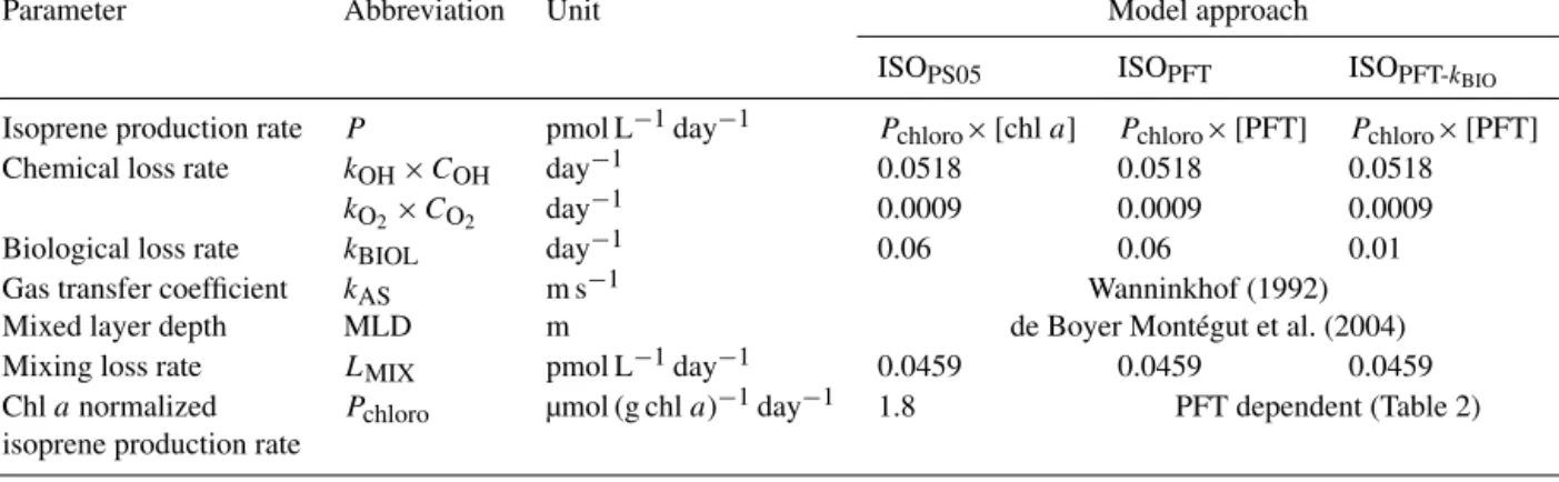
Isoprene was measured in the surface seawater during three separate cruises: the ANT-XXV/1 in the eastern Atlantic Ocean, the SPACES/OASIS cruises in the Indian Ocean, and the ASTRA-OMZ cruise in the eastern Pacific Ocean.

ANT-XXV/1 took place in November 2008 on board the R/VPolarsternfrom Bremerhaven, Germany, to Cape Town, South Africa (Fig. 1; for details about isoprene and ancil- lary data see also Zindler et al., 2014). The SPACES/OASIS cruises took place in June–July 2014 on board the R/VSonne from Durban, South Africa, via Port Louis, Mauritius, to Malé, Maldives, and the ASTRA-OMZ cruise took place in October 2015 on board the R/V Sonnefrom Guayaquil, Ecuador, to Antofagasta, Chile (Fig. 1). Air mass backward trajectories (12 h; starting altitude: 50 m) from the Hybrid Single-Particle Lagrangian Integrated Trajectory (HYSPLIT;

http://www.arl.noaa.gov/HYSPLIT.php) model were calcu- lated for the sampling sites. The trajectories, in combination with atmospheric measurements, suggest that the air masses encountered on these cruises were from over the ocean for more than 12 h prior to sampling and are therefore unlikely to contain significant isoprene derived from terrestrial sources (Fig. 1).

2.3 Isoprene measurements 2.3.1 Eastern Atlantic Ocean

The isoprene measurements from the ANT-XXV/1 (Novem- ber 2008, eastern Atlantic Ocean) cruise are described in de- tail in Zindler et al. (2014). Seawater from approximately

2 m depth was continuously pumped on board and flowed through a porous Teflon membrane equilibrator. Isoprene was equilibrated by using a counterflow of dry air and was measured using an atmospheric pressure chemical ionization mass spectrometer (mini-CIMS), which consists of a ⁶³Ni atmospheric pressure ionization source coupled to a single quadrupole mass analyzer (Stanford Research Systems, SRS RGA200). Isoprene from a standard tank was added to the equilibrated air stream every 12 h to calibrate the system.

The precision for isoprene measurements was±13 %. The isoprene data used here are 5 min averages.

2.3.2 Indian and eastern Pacific Oceans

The isoprene measurements on the SPACES/OASIS (June–

July 2014, Indian Ocean) and ASTRA-OMZ (October 2015, eastern Pacific Ocean) cruises have not been published pre- viously. Water samples (50 mL) were taken every 3 h from a continuously running seawater pump system located in the ship’s moon pool at approximately 6 m depth. All samples were analyzed on board within 15 min of collection using a purge and trap system attached to a gas chromatograph/mass spectrometer operating in single ion mode (GC/MS; Agi- lent 7890A/Agilent 5975C; inert XL MSD with triple axis detector). Isoprene was purged from the water sample with helium for 15 min and dried using a Nafion membrane dryer (Perma Pure; ASTRA-OMZ) or potassium carbonate (SPACES/OASIS). Before being injected into the GC, iso- prene was preconcentrated in a trap cooled with liquid ni- trogen. Gravimetrically prepared liquid standards in ethy- lene glycol were measured in the same way as the sam- ples and used to perform daily calibrations for quantification.

Gaseous deuterated isoprene (isoprene-d5) was measured to- gether with each sample as an internal standard to account for possible sensitivity drift between calibrations. The precision for isoprene measurements was±8 %.

Air samples were collected in electropolished stainless steel flasks and pressurized to approximately 2.5 atm with a metal bellows pump. Analysis was conducted after samples were returned to the laboratory. Isoprene was measured along with a range of halocarbons, hydrocarbons, and other gases using a combined GC/MS/FID/ECD system with a modified Markes Unity II/CIA sample preconcentrator. The modifica- tions incorporated a water removal system consisting of a cold trap (−20^◦C) and a Perma Pure dryer (MD-050-24).

Isoprene and > C4 hydrocarbons were quantified using se- lected ion MS and were calibrated against a whole air sam- ple that is referenced to a NIST hydrocarbon mixture using GC/FID. Precision for isoprene is estimated at approximately

±0.4 ppt+5 %.

84 W 80 W 76 W 72 W ^{o o o o} 24 S ^o

16 S ^o 8 S ^o 0^o

Guayaquil

Antofagasta

20 W ^o 0 ^o 20 E ^o 40^oE 60 E ^o 36 S ^o

18 S ^o 0^o 18 N ^o 36 N ^o 54 N ^o

Bremerhaven

Cape Town Durban

Port Louis Male

Height [m]

20 40 60 80 100 120 140 160 180 200

ASTRA-OMZ

ANT-XXV/1

SPACES/OASIS

Figure 1.Cruise tracks (black) of ANT-XXV/1 (November 2008, eastern Atlantic Ocean), SPACES/OASIS (June–July 2014, Indian Ocean) and ASTRA-OMZ (October 2015, eastern Pacific Ocean). Air mass back trajectories calculated for 12 h with a starting height of 50 m using HYSPLIT are superimposed on the cruise track. Color coding indicates altitude above sea level.

3 Results and discussion

3.1 Comparison of modeled and in situ measured isoprene data

The shipboard isoprene measurements from the ANT-XXV/1 cruise ranged from 2 to 157 pmol L⁻¹, with the highest levels in the subtropics of the Southern Hemisphere and lower lev- els in the tropics (Fig. 2). Model simulations were carried out along the cruise track using monthly mean satellite data from November 2008 for chla, surface winds, SST, and MLD as input parameters. The simulations underestimated the mea- sured isoprene concentrations significantly, by as much as a factor of 20 over most of the cruise track (mean error of 19.1 pmol L⁻¹). Simulations were also carried out using in situ shipboard measurements (chla, wind speed, SST, MLD) as the input parameters. In both cases, the model simulations show a peak in the calculated isoprene levels at 13–17^◦N which is not present in the observations, whereas the peak, using in situ data as input parameter, is much smaller. This peak corresponds to elevated chl aconcentrations, suggest- ing that while there may have been high biological activity in this region, isoprene-producing species were not abundant (Figs. 3, 4). These results demonstrate that a single isoprene production factor and bulk chl a concentration do not ade- quately describe the variability in isoprene production. When isoprene-producing PFTs are dominant, however, the mod- eled isoprene values follow the observed isoprene values (in- creasing isoprene concentration north of 33^◦N; Figs. 2, 5).

The elevated isoprene concentrations in the subtropics of the Southern Hemisphere are not represented by the model.

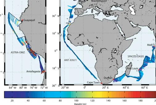
Monthly mean satellite data cannot resolve rapid changes like short phytoplankton blooms or wind events. We com- pared the satellite data to the ship’s in situ measurements of SST, wind speed, calculated MLD, and in situ measured chla concentration as input parameters for the model (Fig. 3) in order to determine if the resolution of the satellite data does resolve important features. The modeled isoprene concentra- tions closely follow the variability in chla, demonstrating that chla has the strongest influence of the four input pa- rameters to the model. The differences between modeled iso- prene concentrations using in situ data vs. satellite data are due primarily to the differences in chla (in situ data are in general 2 times higher than satellite data) with the largest dif- ferences in the regions from 10–25 to 40–45^◦N. As the dis- crepancies between in situ and satellite data are significant, in situ measured data of chlaare used from now on for further calculations with the ISO_PS05 model. Using monthly mean satellite data for wind speed, SST, and climatological values for MLD does not bias the model results significantly relative to the in situ data. Eight-day mean chla and weekly wind speed satellite data (not shown) are also available and could lower the discrepancies to the in situ data. For this study, 8- day values were not useful for this region and time due to cloud coverage (loss of 46 % of data points). A compromise between the two would be to average the 8-day values over a larger area grid to increase the amount of satellite-derived data, but this would lower the resolution and therefore the accurate comparison with the cruise track.

cw isoprene [pmol L−1]

Latitude

−300 −20 −10 0 10 20 30 40 50

10 20 30 40 50 60 150 300

Model (satellite) Model (in situ) Observed

Figure 2.Comparison of observed (black) and modeled seawater isoprene concentrations for the ANT-XXV/1 cruise. Model calculations were carried out using the ISO_PS05model configuration, with monthly mean satellite data (blue) for chla, wind speed, SST, and MLD (climatology) and in situ shipboard measurements (red).

Figure 3.Satellite and in situ data for the ANT-XXV/1 cruise. Monthly mean satellite-derived data (blue) and in situ measurements (red) of (a)chla,(b)wind speed,(c)SST, and(d)monthly mean climatology values (blue) and in situ measurements (red) of MLD.

200

cw isoprene [pmol L−1]

Latitude

−300 −20 −10 0 10 20 30 40 50

10 20 30 40 50 60

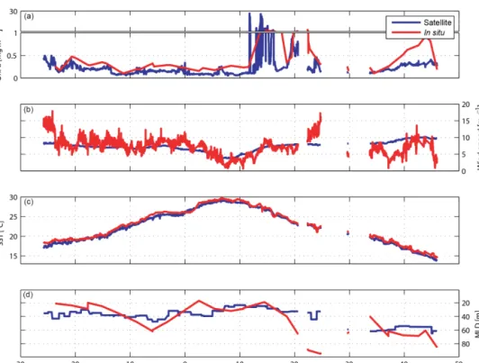
ISO_PS05 Observed ISO_PFT ISO_PFT−kBIO

Figure 4.Comparison of in situ measured isoprene (black) with model-derived isoprene concentrations for the ANT-XXV/1 cruise using ISO_PS05(blue), ISO_PFT(orange), and ISO_PFT-kBIO (red). Squares and circles indicate direct measurements; solid lines are interpolated data.

3.2 Modeling isoprene production using PFTs and revisedk_BIOL

Palmer and Shaw (2005) used a universal Pchloro value of 1.8±0.7 µmoles (g chla)⁻¹day⁻¹based on laboratory phy- toplankton monoculture experiments with several cyanobac- teria, eukaryotes, and coccolithophores (Table 1; Shaw et al., 2003). Subsequent laboratory experiments with mono- cultures of different phytoplankton species have shown gen- erally higher isoprene production rates with large variations between PFTs (Arnold et al., 2009; Bonsang et al., 2010;

Colomb et al., 2008; Exton et al., 2013). In addition, Tran et al. (2013) observed that isoprene concentrations in the field are highly PFT dependent.

We averaged theP_chlorovalues of different PFTs (Table 2) and multiplied these values by the amount of the corre- sponding PFT. Using PFTs instead of total biomass of phy- toplankton (chl a) in the model run results in higher iso- prene model concentrations (orange, Fig. 4), which match the overall isoprene concentration levels measured north of 10^◦N quite well. However, there are also regions where the model still cannot reproduce the measured isoprene con- centrations. Between 10^◦N and 25^◦S, the calculated iso- prene concentrations are quite stable with only small vari- ations between 6 and 23 pmol L⁻¹. Measured concentra- tions are slightly higher between 10^◦N and 12^◦S (15–

30 pmol L⁻¹) and sharply increase to 40–60 pmol L⁻¹south of 12^◦S with a maximum concentration of 150 pmol L⁻¹ (16^◦S). As there were no significant differences in wind

speed, SST, or MLD in these two regions during the cruise, there must be at least one additional source which is not captured in the model. In contrast, at 15^◦N and at 22^◦N the model overestimates the isoprene concentration (Fig. 4).

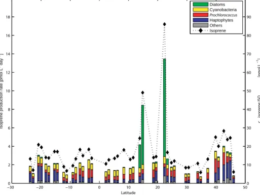
Chlaconcentrations are 10–20 times higher in these two ar- eas than elsewhere on the cruise (Fig. 3) and dominated by diatoms. However, the calculated isoprene is not 10–20 times higher, since diatoms have a relatively low P_chloro value (2.54 µmol (g chla)⁻¹day⁻¹) and, therefore, using their re- spective PFT value modulates the influence of the increased chlaon isoprene concentrations (Fig. 5).

Excluding the two bloom areas, the main PFTs contribut- ing to the modeled isoprene concentrations were prokary- otic phytoplankton (cyanobacteria andProchlorococcus) and haptophytes (Fig. 5, see also Taylor et al., 2011a). It should be noted that the PFTs considered in our study are only part of the full phytoplankton community. In addition, these values can be easily over- or underestimated due to a high variability in the P_chloro values within one group of PFTs (e.g., haptophytes: 1–15.36 µmol isoprene (g chla)⁻¹day⁻¹; Table 2). Using the ISO_PFT-kBIOmodel approach, the isoprene concentrations increase by a factor of 1.35, resulting in bet- ter agreement with the observations (Fig. 4). Overall for the conditions of this cruise, the ISOPFT-k_BIO model simulation yields 12-fold higher isoprene levels than ISOPS05(mean er- ror of 11.8 pmol L⁻¹).

It is obvious that even after implementing these changes the model does not reproduce all the measured isoprene val- ues or their distribution pattern. One particular problem is

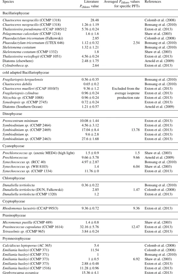
Table 2.Chlorophyll-normalized isoprene production rates (P_chloro) determined from analysis of phytoplankton cultures experiments de- scribed in the literature (Exton et al., 2013 and references therein).P_chlorovalues are given in µmol (g chla)⁻¹day⁻¹.

Species Literature AveragedP_chlorovalues References

P_chlorovalue for specific PFTs Bacillariophyceae

Chaetoceros neogracilis(CCMP 1318) 28.48 Colomb et al. (2008)

Chaetoceros neogracilis(CCMP 1318) 1.26±1.19 Bonsang et al. (2010)

Thalassiosira pseudonana(CCAP 1085/12 5.76±0.24 Exton et al. (2013)

Pelagomonas calceolate(CCMP 1214) 1.6±1.6 Shaw et al. (2003)

Phaeodactylum tricornutum(Falkowski) 2.85 Colomb et al. (2008)

Phaeodactylum tricornutum(UTEX 646) 1.12±0.32 2.54 Bonsang et al. (2010)

Skeletonema costatum 1.32±1.21 Bonsang et al. (2010)

Skeletonema costatum(CCMP 1332) 1.8 Shaw et al. (2003)

Thalassiosira weissflogii(CCMP 1051) 4.56±0.24 Exton et al. (2013)

Diatoms (elsewhere) 2.48±1.75 Arnold et al. (2009)

Cylindrotheca sp. 2.64 Exton et al. (2013)

cold adapted Bacillariophyceae

Fragilariopsis kerguelensis 0.56±0.35 Bonsang et al. (2010)

Chaetoceros debilis 0.65±0.2 Bonsang et al. (2010)

Chaetoceros muelleri(CCAP 1010/3) 9.36±1.2 Excluded from the Exton et al. (2013) Fragilariopsis cylindrus 0.96±0.24 average isoprene Exton et al. (2013) Nitzschia sp.(CCMP 1088) 0.96±0.24 production rate Exton et al. (2013)

Synedropsis sp.(CCMP 2745) 0.72±0.24 Exton et al. (2013)

Diatoms (Southern Ocean) 1.21±0.57 Arnold et al. (2009)

Dinophyceae

Prorocentrum minimum 10.08±1.44 Exton et al. (2013)

Symbiodinium sp.(CCMP 2464) 4.56±3.12 Exton et al. (2013)

Symbiodinium sp.(CCMP 2469) 17.04±8.4 13.78 Exton et al. (2013)

Symbiodinium sp. 9.6±2.8 Exton et al. (2013)

Symbiodinium sp.(CCMP 2463) 27.6±1.68 Exton et al. (2013)

Cyanophyceae

Prochlorococcus sp.(axenic MED4) (high light) 1.5±0.9 1.5 Shaw et al. (2003)

Prochlorococcus 9.66±5.78 9.66 Arnold et al. (2009)

Synechococcus sp.(RCC 40) 4.97±2.87 Bonsang et al. (2010)

Synechococcus sp.(WH 8103) 1.4 6.04 Shaw et al. (2003)

Synechococcus sp.(CCMP 1334) 11.76±0 Exton et al. (2013)

Chlorophyceae

Dunaliella tertiolecta 0.36±0.22 Bonsang et al. (2010)

Dunaliella tertiolecta(DUN, Falkowski) 2.85 1.47 Colomb et al. (2008)

Dunaliella tertiolecta(CCMP 1320) 1.2 Exton et al. (2013)

Cryptophyceae

Rhodomonas lacustris(CCAP 995/3) 9.36±0.72 9.36 Exton et al. (2013) Prasinophyceae

Micromonas pusilla(CCMP 489) 1.4±0.8 Shaw et al. (2003)

Prasinococcus capsulatus(CCMP 1614) 32.16±5.76 12.47 Exton et al. (2013)

Tetraselmis sp.(CCMP 965) 3.84±0.24 Exton et al. (2013)

Prymnesiophyceae

Calcidiscus leptoporus(AC 365) 5.4 Colomb et al. (2008)

Emiliania huxleyi(CCMP 371) 11.54 Colomb et al. (2008)

Emiliania huxleyi(CCMP 371) 1 Bonsang et al. (2010)

Emiliania huxleyi(CCMP 373) 1±0.5 6.92 Shaw et al. (2003)

Emiliania huxleyi(CCMP 373) 2.88±0.48 Exton et al. (2013)

Emiliania huxleyi(CCMP 1516) 11.28±0.96 Exton et al. (2013)

Gephyrocapsa oceanica 15.36±4.1 Exton et al. (2013)

−300 −20 −10 0 10 20 30 40 50 2

4 6 8 10 12 14 16 18 20

Latitude

Isoprene production rate [pmol L day]−1−1

0 10 20 30 40 50 60 70 80 90 100

cw isoprene ISOPFT−kBIO [pmol L−1]

Diatoms Cyanobacteria Prochlorococcus Haptophytes Others Isoprene

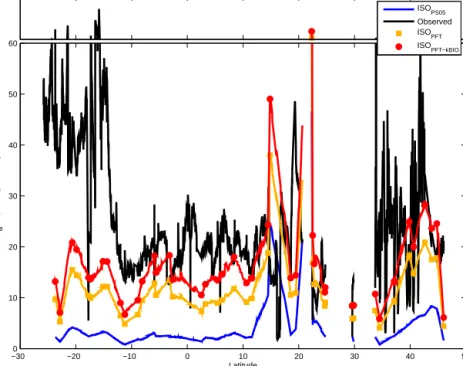
Figure 5.Proportion of main PFTs contributing to the total isoprene production rate for each station during ANT-XXV/1.

that marine isoprene emissions are very low in comparison to terrestrial isoprene emissions. Coastal emissions have to be calculated and interpreted carefully due to this terrestrial in- fluence. We assume no terrestrial influence in the open ocean, since the atmospheric lifetime of isoprene is short. Despite the terrestrial influence on atmospheric isoprene values over the ocean, calculating surface ocean isoprene concentrations, other assumptions in the model should be scrutinized in or- der to understand the discrepancies between measured and calculated values:

1. The model assumes well-mixed isoprene concentra- tions through the MLD, which is, in fact, not the case.

Measurements of depth profiles show a vertical gradi- ent with a maximum of isoprene at the depth of the chl a maximum slightly below the MLD (Bonsang et al., 1992; Milne et al., 1995; Moore and Wang, 2006), which was also measured during our three campaigns (data not shown). Gantt et al. (2009) tried to solve this problem using a light-dependent isoprene production rate, but this resulted in high fluxes in the tropics that are questionable when compared to field measurements.

2. Using PFT-dependent production rates strongly im- proved the model by adding more specific and realistic product information. Nonetheless, we may still be miss- ing some important species within the PFTs, and the average taken over the isoprene measurements among the cultured species within one PFT carries some un- certainty. We used up to eight different PFTs, illus- trating that only the four main groups (haptophytes,

cyanobacteria,Prochlorococcus, and diatoms) produce the most isoprene (Fig. 5). These groups are also the only four detected by the satellite product PHYSAT (Al- vain et al., 2005), which has been used previously for predictions of isoprene (Arnold et al., 2009; Gantt et al., 2009). However, neglecting the other PFTs might lead to different results (others, Fig. 5). This highlights the need to measure the isoprene emission of more species within each PFT group under different physi- ological conditions. Emissions in laboratory culture ex- periments can vary depending on the growth stage of the phytoplankton species (Milne et al., 1995). Shaw et al. (2003) showed that the health conditions of the phy- toplankton species directly influence the emission rates of isoprene when using phage-infected cultures. How- ever, also environmental stress factors, such as tempera- ture and light, influence the ability of different species to produce isoprene (Shaw et al., 2003; Exton et al., 2013;

Meskhidze et al., 2015). More exact data would also, potentially, lower the uncertainty of global marine iso- prene emissions, which was found to be in the range of 20 % when using the upper or lower bounds of PFT- dependent production rates (Gantt et al., 2009).

3. The temporal resolution of the simple model may also not be adequate. Gantt et al. (2009) could show that their model, using remote sensing input in combination with the light dependence of isoprene production, overesti- mated daytime isoprene concentrations and underesti- mated nighttime concentrations compared to the high

temporal resolution field measurements of Matsunaga et al. (2002). The possible diurnal cycle of isoprene could not be resolved with remote sensing data obtained only at a specific local time during the day (e.g., 10:00 for MODIS Terra and 13:00 for MODIS Aqua).

4. The role of bacteria in producing isoprene is also un- clear and may be a missing variable in the steady-state equation. Alvarez et al. (2009) observed bacterial iso- prene production in estuary sediments and discovered isoprene production using different cultures of bacteria.

However, Shaw et al. (2003) could not find any evi- dence of bacterial isoprene production in separate ex- periments.

3.3 Verification of the ISO_PFT-kBIOmodel using data from the Indian and eastern Pacific Oceans

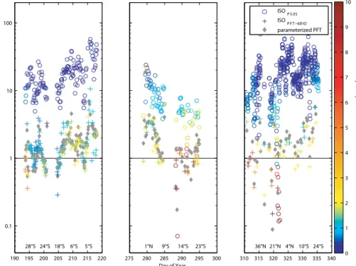
Isoprene concentrations calculated with the original (ISO_PS05) and revised (ISO_PFT-kBIO) model are compared to measured isoprene in the surface ocean at two additional campaigns in two widely differing ocean basins (Indian Ocean, SPACES/OASIS, 2014; eastern Pacific Ocean, ASTRA-OMZ, 2015). The original model ISO_PS05 predicts on average 19±12 times lower isoprene concentrations compared with measured values for the additional two ship campaigns (circles, Fig. 6), which confirms the results ob- tained for ANT-XXV/1. With the newly determined (lower) value for kBIOL and PFT-dependent Pchloro values, the ISOPFT-k_BIO model predicts concentrations that are 10 times higher than the original model ISOPS05 output (crosses, Fig. 6). This leads to a mean underestimation of 1.7±1.2 between modeled and measured isoprene concentrations.

The main cause of the better agreement between mea- sured and modeled isoprene concentrations is the isoprene production rate related to the production input parameter (color coding, Fig. 6). The mean isoprene production rate using chla as an input parameter multiplied by a factor of 1.8 µmol (g chla)⁻¹day⁻¹is less than 0.5 pmol L⁻¹day⁻¹, which is insufficient to explain the measured concentrations in all three campaigns. UsingP_chlorovalues multiplied with the concentration of the related PFT yields in an isoprene production rate of 1–2 pmol L⁻¹day⁻¹in non-bloom areas and even higher rates during phytoplankton blooms, result- ing in isoprene concentrations that are comparable to the measured ones. The opposite can also occur, as seen on DOY 322 (Fig. 6), when PFT specific production rates are smaller than those using chlaonly, due to the dominance of a low isoprene-producing PFT. Even though the improved model is tested in three widely different ocean basins, there are still different regions where the model should be tested with direct isoprene measurements to verify the model output.

4 Global oceanic isoprene emissions and implications for marine aerosol formation

Monthly mean global ocean isoprene concentrations were calculated using the revised model ISO_PFT-kBIO (2^◦×2^◦ grid). As there were no PFT satellite data readily avail- able, we used an empirical relationship between chla and PFTs as parameterized by Hirata et al. (2011). The quality of this parameterization was verified against the PFT data sets from all three campaigns (coefficient of determination:

R²=0.89, Fig. S1 in the Supplement) and is shown in Fig. 6 (grey diamonds). Monthly mean global ocean isoprene emis- sions (Figs. S2–S13 in the Supplement) were averaged in or- der to compute global sea-to-air fluxes of isoprene for 2014 (Fig. 7). An annual emission of 0.21 Tg C was calculated, which is 2 times higher than the value estimated by Palmer and Shaw (2005) (0.11 Tg C yr⁻¹). The highest emissions, more than 100 nmol m⁻²day⁻¹, can be seen in the North At- lantic Ocean and the Southern Ocean, associated with high biological productivity and strong winds driving the air–sea gas exchange. The influence of regional hot spots of biolog- ical productivity, such as the upwelling off Mauretania or the Brazil–Malvinas Confluence Zone, can also be seen. The tropics (23.5^◦S–23.5^◦N) account for only 28 % of global isoprene emissions, but they represent∼47 % of the world oceans.

Yearly emissions of 0.21 Tg C are at the lower end of the range of previously published studies (Arnold et al., 2009, 0.27 Tg C yr⁻¹; Gantt et al., 2009, 0.92 Tg C yr⁻¹).

Both studies use remotely sensed PFT data instead of chlato evaluate the isoprene production. Unlike this study, they im- plemented the Alvain et al. (2005) approach using PHYSAT data, which uses spectral information to produce global distributions of the dominant PFT but is limited to four phytoplankton groups (haptophytes,Prochlorococcus,Syne- chococcus, and diatoms). It should be noted that PHYSAT does not provide actual concentrations but rather only the rel- ative dominance of the four groups. Arnold et al. (2009) used similar assumptions as Palmer and Shaw (2005) to calculate isoprene loss, namely that loss in the water column by advec- tive mixing and aqueous oxidation is on a longer timescale than loss by air–sea gas exchange and, therefore, negligible.

Thus, their calculated emissions of 0.27 Tg C yr⁻¹are an up- per estimate. The approach of Gantt et al. (2009) had two main differences compared to our study. (1) Instead of using the MLD climatology of de Boyer Montégut et al. (2004), they used a maximum depth where isoprene production can occur as calculated by the downwelling irradiance (using the diffuse attenuation coefficient values at 490 nm) and the light propagation throughout the water column that is estimated by using the Lambert–Beer law. (2) They tested two of the detectable PFTs in laboratory experiments using monocul- tures of diatoms and coccolithophores growing under differ- ent light conditions to evaluate light-intensity-dependent iso- prene production rates. Light-intensity-dependent production

190 195 200 205 210 215 220 0.1

1 10 100

2014

cw observed / cw model

310 315 320 325 330 335 340 2008

275 280 285 290 295 300 Day of Year

2015

isoprene production rate [pmol L−1 day−1]

0 1 2 3 4 5 6 7 8 9 10 ISO_{P S 05}

ISOP F T −kB IO parameterized PFT

28°S 24°S 18°S 6°S 5°S 1°N 9°S 14°S 23°S 36°N 21°N 4°N 10°S 24°S

Figure 6.Observed isoprene concentration divided by modeled isoprene concentration on a logarithmic scale for three different cruises: on the left is SPACES/OASIS 2014, in the middle is ASTRA-OMZ 2015, and on the right is ANT-XXV/1 2008. Circles and crosses represent data derived by the original ISO_PS05and revised ISO_PFT-kBIO model, respectively. Every data point is color coded with the corresponding isoprene production rate input parameter. Grey diamonds represent data using parameterized PFT data by Hirata et al. (2011); the black line represents a ratio of 1.

180^o W 120^o W 60^o W 0^o 60^o E 120^o E 180^o W 80^o S

40^o S 0^o 40^o N 80^o N

Isoprene flux [nmol m day ]^{−2 −1}

0 10 20 30 40 50 60 70 80 90 >100

Figure 7.Global marine isoprene fluxes in nmol m⁻²day⁻¹for 2014.

rates of Prochlorococcusand Synechococcus were derived after Gantt et al. (2009) using the original production rates at a specified wavelength measured by Shaw et al. (2003). Their isoprene emission calculations are more than 4 times higher than calculated with our approach, probably as a result of the light-dependent isoprene production rates. Whereas our

global map shows very low emissions in the tropics due to a low phytoplankton productivity, the emissions modeled by Gantt et al. (2009) are comparable to those of high produc- tivity areas like the Southern Ocean or the North Atlantic Ocean, likely as a consequence of the high solar radiation in the tropics. The data from our three cruises contradict this

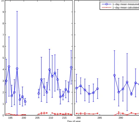
195 200 205 210 215 0

1 2 3 4 5 6 7 8 9 10

2014

Day of year cair isoprene [ppt]

280 285 290 295

2015

1−day mean measured 1−day mean calculated

Figure 8.One-day mean measured (blue) and calculated (red) daytime isoprene mixing ratios (ppt) during SPACES/OASIS (2014) and ASTRA-OMZ (2015). Calculated isoprene air values were derived by using the sea-to-air flux, a marine boundary layer height of 800 m, and the 1 h atmospheric lifetime based on a simple box model approach for each individual measurement.

model-derived result and show very low concentrations in the tropical regions, which implies a very low flux of isoprene to the atmosphere. Furthermore, Meskhidze et al. (2015) showed that, at a specific light intensity, the isoprene pro- duction rate of tested monocultures sharply decreases.

Using atmospheric isoprene concentrations measured in two of the three campaigns, we were able to use a top-down approach to calculate isoprene emissions in order to com- pare with the bottom-up flux estimates. We used a box model with an assumed marine boundary layer height (MBLH) of 800 m, which reflected the local conditions during the two campaigns. The only source of isoprene for the air was as- sumed to be the sea-to-air flux (emission) and the atmo- spheric lifetime (τ) was assumed to be determined by reac- tion with OH (chemical loss, 1 h). The sea-to-air flux was calculated by multiplying kAS with the measured isoprene concentration (CW) in the ocean (Eq. 3). We assumed CA

to be zero in order to have the highest possible sea-to-air- flux, following a conservative approach. The concentration outside the box was assumed to be the same as inside to ne- glect advection into and out of the box. The resulting calcu- lated steady-state isoprene air concentration for every box (1- day mean value of all individual measurements at daytime) is shown in Fig. 8 (for a 1 h lifetime it takes approximately 10 h to achieve steady state) and is calculated as follows:

CA=(kAS×CW) τ

MBLH. (5)

For comparison, the mean measured concentration of isoprene in the atmosphere during the two cruises is 2.5±1.5 ppt and therefore 45 times higher than the calcu- lated isoprene air values. The measured concentrations match previously measured remote open ocean atmospheric val- ues (Shaw et al., 2003). We only used atmospheric measure- ments which were obtained during daytime (to reflect reac- tion with OH) and were not influenced by terrestrial sources.

This was determined by omitting data points with con- comitant high levels of anthropogenic hydrocarbons (con- centrations of butane higher 20 ppt). Reported mean at- mospheric lifetime estimates of isoprene range from min- utes up to 4 h, depending mainly on the atmospheric con- centration of OH (Pfister et al., 2008). We calculate that for an estimated lifetime of 1 and 4 h, a sea-to-air flux of at least 2000 and 500 nmol m⁻²day⁻¹, respectively, is needed to reach the atmospheric concentration measured dur- ing SPACES/OASIS and ASTRA-OMZ, which is approxi- mately 10–20 times higher than computed (even when as- suming C_A as zero). Recent studies showed that the mea- sured fluxes of isoprene range from 4.6–148 nmol m⁻²day⁻¹ in June–July 2010 in the Arctic (Tran et al., 2013) to 181.0–

313.1 nmol m⁻²day⁻¹ in the productive Southern Ocean

during austral summer 2010/2011 (Kameyama et al., 2014).

Despite these high literature values, it appears that the cal- culated fluxes cannot explain the measured atmospheric con- centrations even when a conservative lifetime of 4 h is as- sumed.

5 Conclusions

The revised Palmer and Shaw (2005) isoprene emission model was evaluated against direct surface ocean isoprene measurements from three different ocean basins, yielding comparable ocean concentrations that were slightly under- estimated (factor of 1.7±1.2). The resulting annual global oceanic isoprene emissions are 2 times higher than the cal- culated flux with the original model. However, using a sim- ple top-down approach based on measured atmospheric iso- prene levels, we calculate that emissions from the ocean are required to be more than 1 order of magnitude greater than those computed using the bottom-up estimate based on mea- sured oceanic isoprene levels. This result is consistent with a numerical evaluation of global ocean isoprene emissions by Luo and Yu (2010). One possible explanation could be production in the surface microlayer (SML) that is not simu- lated by the model. Ciuraru et al. (2015) showed that isoprene is produced photochemically by surfactants in an organic monolayer at the air–sea interface. As the SML is enriched with surfactants (Wurl et al., 2011), the isoprene flux from the SML could range from 1000 to 33 000 nmol m⁻²day⁻¹, which is much larger (about 2 orders of magnitude) than the highest fluxes calculated from our observations. To date, there is no evidence of such a large gradient in the surface ocean between the surface and 10 m. Thus, further field mea- surements probing the SML could be a step forward in recon- ciling the role of the ocean for the atmospheric isoprene bud- get. Using the bottom-up approach, isoprene emissions are much smaller and given this scenario, isoprene consequently appears to be a relatively insignificant source of OC in the remote marine atmosphere. Arnold et al. (2009) calculated a yield of 0.04 Tg yr⁻¹OC derived from marine isoprene by using yearly emissions of 1.9 Tg yr⁻¹and a SOA yield of 2 % (Henze and Seinfeld, 2006). This is equivalent to 0.5 % of es- timated 8 Tg yr⁻¹global source of oceanic OC (Spracklen et al., 2008). Using our bottom-up emission of 0.21 Tg C yr⁻¹ will even lower this small influence. Until this discrepancy between bottom-up and top-down approaches is resolved, the question of whether isoprene is a main precursor to remote marine boundary layer particle formation still remains open.

6 Data availability

All isoprene data are available from the corresponding au- thor. Pigment data from ANT-XXV/1 are available from PANGAEA (Taylor et al., 2011b). Pigment data from SPACES/OASIS and ASTRA-OMZ will be available from

PANGAEA but for now can be obtained through the corre- sponding author.

The Supplement related to this article is available online at doi:10.5194/acp-16-11807-2016-supplement.

Acknowledgements. The authors would like to thank the cap- tain and crew of the R/V Polarstern (ANT-XXV/1) and R/V Sonne(SPACES/OASIS and ASTRA-OMZ) as well as the chief scientists, Gerhard Kattner (ANT-XXV/1) and Kirstin Krüger (SPACES/OASIS). Boris Koch and Birgit Quack also pro- vided valuable help. We thank Sonja Wiegmann for HPLC pigment analysis of SPACES/OASIS and ASTRA-OMZ samples, Sonja Wiegmann and Wee Cheah for pigment sampling during SPACES/OASIS, and Rüdiger Röttgers for helping with pigment sampling during ASTRA-OMZ. Paul I. Palmer gratefully ac- knowledges his Royal Society Wolfson Research Merit Award.

Elliot Atlas acknowledges support from the NASA UARP program and thanks Leslie Pope and Xiaorong Zhu for assistance in canister preparation. The authors gratefully acknowledge the NOAA Air Resources Laboratory (ARL) for the provision of the HYSPLIT transport and dispersion model used in this publication as well as NASA for providing the satellite MODIS Aqua and MODIS Terra data. QuikScat and SeaWinds data were produced by Remote Sens- ing Systems with thanks to the NASA Ocean Vector Winds Science Team for funding and support. This work was carried out under the Helmholtz Young Investigator Group of Christa A. Marandino, TRASE-EC (VH-NG-819), from the Helmholtz Association through the President’s Initiative and Networking Fund and the GEOMAR Helmholtz Centre for Ocean Research Kiel. The R/V Sonnecruises SPACES/OASIS and ASTRA-OMZ were financed by the BMBF through grants 03G0235A and 03G0243A, respec- tively.

The article processing charges for this open-access publication were covered by a Research

Centre of the Helmholtz Association.

Edited by: A. Hofzumahaus

Reviewed by: two anonymous referees

References

Aiken, J., Pradhan, Y., Barlow, R., Lavender, S., Poulton, A., Holligan, P., and Hardman-Mountford, N.: Phytoplankton pig- ments and functional types in the Atlantic Ocean: A decadal assessment, 1995–2005, Deep-Sea Res. Pt. II, 56, 899–917, doi:10.1016/j.dsr2.2008.09.017, 2009.

Alvain, S., Moulin, C., Dandonneau, Y., and Breon, F. M.: Re- mote sensing of phytoplankton groups in case 1 waters from global SeaWiFS imagery, Deep-Sea Res. Pt. I, 52, 1989–2004, doi:10.1016/j.dsr.2005.06.015, 2005.

Alvarez, L. A., Exton, D. A., Timmis, K. N., Suggett, D. J., and McGenity, T. J.: Characterization of marine isoprene-

degrading communities, Environ. Microbiol., 11, 3280–3291, doi:10.1111/j.1462-2920.2009.02069.x, 2009.

Andreae, M. O. and Rosenfeld, D.: Aerosol–cloud–

precipitation interactions. Part 1. The nature and sources of cloud-active aerosols, Earth-Sci. Rev., 89, 13–41, doi:10.1016/j.earscirev.2008.03.001, 2008.

Anttila, T., Langmann, B., Varghese, S., and O’Dowd, C.: Contribu- tion of Isoprene Oxidation Products to Marine Aerosol over the North-East Atlantic, Advances in Meteorology, 2010, 482603, doi:10.1155/2010/482603, 2010.

Arneth, A., Monson, R. K., Schurgers, G., Niinemets, Ü., and Palmer, P. I.: Why are estimates of global terrestrial isoprene emissions so similar (and why is this not so for monoterpenes)?, Atmos. Chem. Phys., 8, 4605–4620, doi:10.5194/acp-8-4605- 2008, 2008.

Arnold, S. R., Spracklen, D. V., Williams, J., Yassaa, N., Sciare, J., Bonsang, B., Gros, V., Peeken, I., Lewis, A. C., Alvain, S., and Moulin, C.: Evaluation of the global oceanic isoprene source and its impacts on marine organic carbon aerosol, Atmos. Chem.

Phys., 9, 1253–1262, doi:10.5194/acp-9-1253-2009, 2009.

Atkinson, R. and Arey, J.: Atmospheric degradation of volatile or- ganic compounds, Chem. Rev., 103, 4605–4638, 2003.

Baker, A. R., Turner, S. M., Broadgate, W. J., Thompson, A., Mc- Figgans, G. B., Vesperini, O., Nightingale, P. D., Liss, P. S., and Jickells, T. D.: Distribution and sea-air fluxes of biogenic trace gases in the eastern Atlantic Ocean, Global Biogeochem. Cy., 14, 871–886, doi:10.1029/1999gb001219, 2000.

Barlow, R. G., Cummings, D. G., and Gibb, S. W.: Improved resolution of mono- and divinyl chlorophylls a and b and zeaxanthin and lutein in phytoplankton extracts using re- verse phase C-8 HPLC, Mar. Ecol.-Prog. Ser., 161, 303–307, doi:10.3354/meps161303, 1997.

Bonsang, B., Polle, C., and Lambert, G.: Evidence for Marine Production of Isoprene, Geophys. Res. Lett., 19, 1129–1132, doi:10.1029/92gl00083, 1992.

Bonsang, B., Gros, V., Peeken, I., Yassaa, N., Bluhm, K., Zoellner, E., Sarda-Esteve, R., and Williams, J.: Isoprene emission from phytoplankton monocultures: the relationship with chlorophylla, cell volume and carbon content, Environ. Chem., 7, 554–563, doi:10.1071/EN09156, 2010.

Broadgate, W. J., Liss, P. S., and Penkett, S. A.: Seasonal emissions of isoprene and other reactive hydrocarbon gases from the ocean, Geophys. Res. Lett., 24, 2675–2678, doi:10.1029/97gl02736, 1997.

Broadgate, W. J., Malin, G., Kupper, F. C., Thompson, A., and Liss, P. S.: Isoprene and other non-methane hydrocarbons from sea- weeds: a source of reactive hydrocarbons to the atmosphere, Mar.

Chem., 88, 61–73, doi:10.1016/j.marchem.2004.03.002, 2004.

Carlton, A. G., Wiedinmyer, C., and Kroll, J. H.: A review of Sec- ondary Organic Aerosol (SOA) formation from isoprene, At- mos. Chem. Phys., 9, 4987–5005, doi:10.5194/acp-9-4987-2009, 2009.

Charlson, R. J., Lovelock, J. E., Andreae, M. O., and Warren, S.

G.: Oceanic phytoplankton, atmospheric sulfur, cloud albedo and climate, Nature, 326, 655–661, doi:10.1038/326655a0, 1987.

Ciuraru, R., Fine, L., Pinxteren, M. V., D’Anna, B., Herrmann, H., and George, C.: Unravelling New Processes at Interfaces: Pho- tochemical Isoprene Production at the Sea Surface, Environ. Sci.

Technol., 49, 13199–13205, doi:10.1021/acs.est.5b02388, 2015.

Colomb, A., Yassaa, N., Williams, J., Peeken, I., and Lochte, K.:

Screening volatile organic compounds (VOCs) emissions from five marine phytoplankton species by head space gas chromatog- raphy/mass spectrometry (HS-GC/MS), J. Environ. Monitor., 10, 325–330, doi:10.1039/b715312k, 2008.

de Boyer Montégut, C., Madec, G., Fischer, A. S., Lazar, A., and Iu- dicone, D.: Mixed layer depth over the global ocean: An exam- ination of profile data and a profile-based climatology, J. Geo- phys. Res.-Oceans, 109, C12003, doi:10.1029/2004JC002378, 2004.

de Leeuw, G., Andreas, E. L., Anguelova, M. D., Fairall, C. W., Lewis, E. R., O’Dowd, C., Schulz, M., and Schwartz, S. E.: Pro- duction flux of sea spray aerosol, Rev. Geophys., 49, RG2001, doi:10.1029/2010RG000349, 2011.

Ekström, S., Nozière, B., and Hansson, H.-C.: The Cloud Con- densation Nuclei (CCN) properties of 2-methyltetrols and C3- C6 polyols from osmolality and surface tension measurements, Atmos. Chem. Phys., 9, 973–980, doi:10.5194/acp-9-973-2009, 2009.

Exton, D. A., Suggett, D. J., McGenity, T. J., and Steinke, M.:

Chlorophyll-normalized isoprene production in laboratory cul- tures of marine microalgae and implications for global models, Limnol. Oceanogr., 58, 1301–1311, 2013.

Gantt, B., Meskhidze, N., and Kamykowski, D.: A new physically- based quantification of marine isoprene and primary or- ganic aerosol emissions, Atmos. Chem. Phys., 9, 4915–4927, doi:10.5194/acp-9-4915-2009, 2009.

Guenther, A., Karl, T., Harley, P., Wiedinmyer, C., Palmer, P. I., and Geron, C.: Estimates of global terrestrial isoprene emissions using MEGAN (Model of Emissions of Gases and Aerosols from Nature), Atmos. Chem. Phys., 6, 3181–3210, doi:10.5194/acp-6- 3181-2006, 2006.

Henze, D. K. and Seinfeld, J. H.: Global secondary organic aerosol from isoprene oxidation, Geophys. Res. Lett., 33, L09812, doi:10.1029/2006gl025976, 2006.

Hirata, T., Hardman-Mountford, N. J., Brewin, R. J. W., Aiken, J., Barlow, R., Suzuki, K., Isada, T., Howell, E., Hashioka, T., Noguchi-Aita, M., and Yamanaka, Y.: Synoptic relationships be- tween surface Chlorophylla and diagnostic pigments specific to phytoplankton functional types, Biogeosciences, 8, 311–327, doi:10.5194/bg-8-311-2011, 2011.

Hu, Q.-H., Xie, Z.-Q., Wang, X.-M., Kang, H., He, Q.-F., and Zhang, P.: Secondary organic aerosols over oceans via oxidation of isoprene and monoterpenes from Arctic to Antarctic, Supple- ment, Scientific Reports, 3, 2280, doi:10.1038/srep02280, 2013.

Kameyama, S., Yoshida, S., Tanimoto, H., Inomata, S., Suzuki, K., and Yoshikawa-Inoue, H.: High-resolution observations of dissolved isoprene in surface seawater in the Southern Ocean during austral summer 2010–2011, J. Oceanogr., 70, 225–239, doi:10.1007/s10872-014-0226-8, 2014.

Lana, A., Simó, R., Vallina, S. M., and Dachs, J.: Potential for a biogenic influence on cloud microphysics over the ocean: a cor- relation study with satellite-derived data, Atmos. Chem. Phys., 12, 7977–7993, doi:10.5194/acp-12-7977-2012, 2012.

Lelieveld, J., Butler, T. M., Crowley, J. N., Dillon, T. J., Fischer, H., Ganzeveld, L., Harder, H., Lawrence, M. G., Martinez, M., Taraborrelli, D., and Williams, J.: Atmospheric oxidation capac- ity sustained by a tropical forest, Supplement, Nature, 452, 737–

740, doi:10.1038/nature06870, 2008.