Modelling marine emissions and atmospheric distributions of

(1)

doi:10.5194/acp-15-11753-2015

Modelling marine emissions and atmospheric distributions of

halocarbons and dimethyl sulfide: the influence of prescribed water concentration vs. prescribed emissions

S. T. Lennartz¹, G. Krysztofiak^2,a, C. A. Marandino¹, B.-M. Sinnhuber², S. Tegtmeier¹, F. Ziska¹, R. Hossaini³, K. Krüger⁴, S. A. Montzka⁵, E. Atlas⁶, D. E. Oram⁷, T. Keber⁸, H. Bönisch⁸, and B. Quack¹

1GEOMAR Helmholtz-Centre for Ocean Research Kiel, Kiel, Germany

2Karlsruhe Institute of Technology, Institute for Meteorology and Climate Research, Karlsruhe, Germany

3School of Earth and Environment, University of Leeds, Leeds, UK

4University of Oslo, Department of Geosciences, Oslo, Norway

5NOAA/CMDL, Boulder, CO, USA

6RSMAS/MAC, University of Miami, Florida, USA

7National Centre for Atmospheric Science, Centre for Oceanography and Atmospheric Science, University of East Anglia, Norwich, UK

8Goethe University Frankfurt a. M., Institute for Atmospheric and Environmental Sciences, Frankfurt, Germany

anow at: LPC2E, UMR 7328, CNRS-Université d’Orléans, 45071 Orléans CEDEX 2, France Correspondence to: S. T. Lennartz (slennartz@geomar.de)

Received: 24 April 2015 – Published in Atmos. Chem. Phys. Discuss.: 30 June 2015 Revised: 23 September 2015 – Accepted: 30 September 2015 – Published: 22 October 2015

Abstract. Marine-produced short-lived trace gases such as dibromomethane (CH₂Br₂), bromoform (CHBr₃), methyliodide (CH₃I) and dimethyl sulfide (DMS) significantly impact tropospheric and stratospheric chemistry. Describing their marine emissions in atmospheric chemistry models as accurately as possible is necessary to quantify their impact on ozone depletion and Earth’s radiative budget. So far, marine emissions of trace gases have mainly been prescribed from emission climatologies, thus lacking the inter- action between the actual state of the atmosphere and the ocean. Here we present simulations with the chemistry climate model EMAC (ECHAM5/MESSy Atmospheric Chem- istry) with online calculation of emissions based on surface water concentrations, in contrast to directly prescribed emissions. Considering the actual state of the model atmosphere results in a concentration gradient consistent with model real- time conditions at the ocean surface and in the atmosphere, which determine the direction and magnitude of the com- puted flux. This method has a number of conceptual and practical benefits, as the modelled emission can respond consistently to changes in sea surface temperature, surface wind

speed, sea ice cover and especially atmospheric mixing ratio. This online calculation could enhance, dampen or even invert the fluxes (i.e. deposition instead of emissions) of very short-lived substances (VSLS). We show that differences between prescribing emissions and prescribing concentrations (−28 % for CH₂Br₂to+11 % for CHBr₃)result mainly from consideration of the actual, time-varying state of the atmosphere. The absolute magnitude of the differences depends mainly on the surface ocean saturation of each particular gas.

Comparison to observations from aircraft, ships and ground stations reveals that computing the air–sea flux interactively leads in most of the cases to more accurate atmospheric mixing ratios in the model compared to the computation from prescribed emissions. Calculating emissions online also enables effective testing of different air–sea transfer velocity (k)parameterizations, which was performed here for eight different parameterizations. The testing of these differentk values is of special interest for DMS, as recently published parameterizations derived by direct flux measurements using eddy covariance measurements suggest decreasingkvalues at high wind speeds or a linear relationship with wind speed.

(2)

Implementing these parameterizations reduces discrepancies in modelled DMS atmospheric mixing ratios and observations by a factor of 1.5 compared to parameterizations with a quadratic or cubic relationship to wind speed.

1 Introduction

The oceans emit large amounts of halogen- (Penkett et al., 1985; Quack and Wallace, 2003) and sulfur-containing substances (Bates et al., 1992; Watts, 2000) that influence atmospheric chemistry. Organic bromine and iodine in the atmosphere is largely supplied by oceanic emissions of very short- lived substances (VSLS) such as dibromomethane (CH2Br2), bromoform (CHBr3) and methyliodide (CH3I) (Lovelock and Maggs, 1973; Hossaini et al., 2013). Also, a large fraction of the atmospheric sulfur loading is due to oceanic emissions of OCS, CS₂, H₂S and dimethyl sulfide (DMS;

CH₃SCH₃), the latter being the major compound transport- ing sulfur from the ocean to the atmosphere (Watts, 2000;

Sheng et al., 2015). Thus, we focus on DMS in this study.

Assessing marine emissions of VSLS is crucial, as they significantly influence Earth’s atmosphere in both the troposphere and the stratosphere. In the troposphere, bromine- containing VSLS such as CHBr₃ and CH₂Br₂ contribute to ozone destruction and alter the oxidative capacity (von Glasow et al., 2004; Salawitch, 2006). Oceanic CH3I is the main organic iodine compound in the atmosphere (Lovelock and Maggs, 1973) and impacts tropospheric oxidative capacity and ozone destruction (Chameides and Davis, 1980;

Saiz-Lopez et al., 2012). Iodine oxides, which can be product gases of CH₃I are likely to contribute to nucleation and growth of secondary marine aerosol production (O’Dowd and De Leeuw, 2007). DMS emitted to the troposphere is a precursor of secondary organic aerosol and potentially cloud condensation nuclei and thus influences the radiative budget (Charlson et al., 1987). Halogenated VSLS also enhance stratospheric ozone depletion (Sinnhuber and Meul, 2015) and thus contribute to the ozone-driven radiative forc- ing of climate (Hossaini et al., 2015). Despite the short lifetime of CH3I (4–7 days) compared to the bromocarbons (6–

120 days), there is potential for a small fraction of marine- produced CH3I to be transported to the stratosphere where it also contributes to ozone depletion (Tegtmeier et al., 2013;

Solomon et al., 1994). DMS has a shorter lifetime of 11 min–

46 h (Barnes et al., 2006; Osthoff et al., 2009) compared to CH₃I. Despite the short lifetime, there is potential even for the very short-lived DMS to be transported to the tropical tropopause layer (TTL) in convective hot spot regions (Marandino et al., 2013a, b).

The impact of marine VSLS emissions on atmospheric chemistry has been studied in chemistry–climate and transport models (e.g. Salawitch et al., 2005; Kerkweg et al., 2006b; Sinnhuber et al., 2009; Liang et al., 2010; Ordóñez et al., 2012). Therein, marine emissions of the VSLS have

mainly been based on prescribed boundary layer mixing ratios (Aschmann et al., 2009) or emission scenarios (Warwick et al., 2006; Liang et al., 2010; Ordóñez et al., 2012; Hossaini et al., 2013). However, prescribing emissions in atmospheric models lacks the impact of the atmospheric boundary layer mixing ratio on the concentration gradient. This concentration gradient at the interface between ocean and atmosphere directly influences the emissions, as it determines the direction and magnitude of the flux. The lack of potential feed- backs can result in a modelled atmospheric surface concentration inconsistent with the oceanic surface concentration.

Here, we evaluate a conceptually different way of considering marine emissions in chemical climate models that is based on a consistent concentration gradient between ocean and atmosphere. In contrast to previous approaches of either specifying atmospheric surface mixing ratios or specifying sea-to-air fluxes, water concentrations are prescribed and emissions are calculated online. Thus, the concentration gradient at the interface and the emissions are consistent with the atmospheric boundary layer and the ocean surface, and the emissions can respond to the actual state of the atmosphere. The approach is applied to established concentration climatologies of short-lived halocarbons (CH₂Br₂, CHBr₃, CH₃I) and sulfur compounds (DMS) that share com- mon characteristics such as supersaturation in the surface ocean and marine production. For the halocarbons, this set- up is applied for the first time and uses surface ocean concentration climatologies derived from observations by Ziska et al. (2013). Oceanic DMS emissions have been evaluated in coupled ocean–atmosphere models (Kloster et al., 2006;

Cameron-Smith et al., 2011) or modelled online during a test for the implementation of different submodels (Kerkweg et al., 2006b). In our study, the focus lies on how to consider oceanic emissions in a stand-alone atmospheric model, and uses the most updated DMS concentrations available (Lana et al., 2011). Additionally, we compare the output of the two methods with observations from aircraft and ship campaigns.

Prescribing water concentrations and calculating emissions online enables convenient testing of different air–sea gas exchange parameterizations. Air–sea gas exchange is calculated as the product of the concentration gradient between air and water at the surface and the transfer velocity. The latter needs to be parameterized, and many different parameterizations have been published (see e.g. Wanninkhof et al., 2009 for a summary). Most parameterizations relate the transfer velocity to wind speed (e.g. Liss and Merlivat, 1986; Wan- ninkhof and McGillis, 1999; Nightingale et al., 2000; Ho et al., 2006), but others take the effect of bubble-mediated transfer (Asher and Wanninkhof, 1998) or enhancement by rain (Ho et al., 1997, 2004) into account. Testing a variety of different parameterizations on prescribed water concentrations to calculate atmospheric abundances provides information on the uncertainties of global emission estimates.

The experimental set-up consists of two steps. First, we prescribed surface water concentrations in the chemistry cli-

(3)

mate model EMAC (ECHAM5/MESSy Atmospheric Chem- istry) (Jöckel et al., 2006, 2010) and air–sea exchange of VSLS was then calculated online by the submodel AIRSEA (Pozzer et al., 2006). The model results are then evaluated and compared to a simulation where the difference results from prescribed VSLS emissions (PE). To compare the simulation set-up with prescribed emissions to the set-up with prescribed water concentrations, we used the same concentration climatologies that were used to create the emission climatologies. In our study, these concentration and corresponding emission climatologies were published by Ziska et al. (2013) for the halocarbons and Lana et al. (2011) for DMS. The modelled atmospheric mixing ratios of the gases are compared to measurements from time series of ground- based stations, ship and aircraft campaigns in order to identify whether the online calculation is simulating the atmospheric mixing ratios more accurately. In a second step, we use the coupled module to test the sensitivity of the global emissions to eight different, frequently used or recently published, transfer velocity parameterizations.

2 Model set-up and data description

2.1 The atmosphere-chemistry model EMAC

The EMAC model is a global atmospheric chemistry climate model described in Jöckel et al. (2006, 2010).

ECHAM5/MESSy includes submodels describing processes of the troposphere and middle atmosphere as well as interac- tion with land and human influences. Air–sea gas exchange is calculated in EMAC with the submodule AIRSEA, as described by Pozzer et al. (2006).

The numerical simulations were nudged towards the European Centre for Medium-Range Weather Forecasts (ECMWF) ERA-Interim reanalysis (Dee et al., 2011) every 6 h (temperature, divergence, vorticity, surface pressure). The resolution of the EMAC atmosphere was∼2.8^◦×2.8^◦(T42) and 39 vertical hybrid pressure levels up to 0.01 hPa (L39).

The effect of resolution on the results tested with a finer resolution (T106) was only minor (see Table S2 in the Sup- plement). The atmospheric model as well as the submodel AIRSEA uses a time step of 600 s. The convective transport follows the scheme of Tiedtke (1989) and the tracer advec- tion is described in Lin and Rood (1996). An overview of these nudged simulation set-ups can be found in Sect. 2.3.

The simulations include the four very short-lived species, CH₂Br₂, CHBr₃, CH₃I and DMS, and simplified atmospheric loss reactions for them. The loss reactions include

– oxidation with OH, O(¹D), Cl and photolysis for CHBr₃ and CH₂Br₂following the reactions rates by Sander et al. (2011);

– oxidation with OH, Cl and photolysis for CH₃I (Sander et al., 2011);

– and oxidation with OH and O(³P) for DMS (Sander et al., 2011).

EMAC uses monthly mean concentrations of OH, devel- oped and evaluated for the TransCom-CH4 model intercomparison project, and discussed in detail by Patra et al. (2014).

Monthly mean photolysis rates for VSLS were calculated by the TOMCAT CTM (chemical transport model) which has been used extensively to examine the tropospheric chemistry of VSLS (e.g. Hossaini et al., 2013). These fields were provided at a horizontal resolution of 2.8^◦×2.8^◦ (longitude×latitude) and on 60 vertical levels (surface to

∼60 km). TOMCAT calculates photolysis rates online using the code of Hough (1988) which considers both direct and scattered radiation. Within TOMCAT, this scheme is supplied with surface albedo, monthly mean climatolog- ical cloud fields and ozone and temperature profiles. The photolysis rates have recently been used and evaluated as part of the ongoing TransCom-VSLS model intercomparison project (http://www.transcom-vsls.com).

The simulated atmospheric lifetimes in our set-up gener- ally agree well with published estimates for these gases, indicating that the basic assumption of the simplified chemistry applied here is valid. The local mean tropical (20^◦N–20^◦S) lifetime of CH₂Br₂in the troposphere in our model study is 143 days and thus lies below 167 days, which was found in Hossaini et al. (2010). The mean tropospheric tropical lifetime of CHBr3 is 20 days in our study, which is consistent within 10 % with a recent reevaluation of CHBr3lifetime by Papanastasiou et al. (2014), together with a recent reevaluation of the reaction of OH with CHBr₃by Orkin et al. (2013).

The local lifetime of CH₃I in our study is 3 days, which is in accordance with the study of Tegtmeier et al. (2013). The tropical lifetime of DMS in our study ranges between less than 1 day and up to 3 days and is thus within but at the higher end of the range of 11 min–46 h (Barnes et al., 2006;

Osthoff et al., 2009).

2.2 Parameterizations of air-sea gas exchange

In this study, the AIRSEA submodel (Pozzer et al., 2006) and its approach for air–sea gas exchange was adopted, using the two-layer model (Liss and Slater, 1974). Marine emissions (F) of gases are calculated as the product of the concentration gradient between air and water concentration of the gas (1c)and the transfer velocity (k; Eq. 1), which needs to be parameterized.

F =k·1c=k·(c_w−H·c_air) (1) withc_wbeing the water concentration,Hthe Henry constant (dimensionless, water over air) andc_airthe concentration of the gas in air which was taken from the modelled atmosphere in the respective time step. Henry constants and their temperature dependencies are taken from Moore et al. (1995) for the halocarbons and De Bruyn et al. (1995) for DMS.

(4)

The transfer velocitykcomprises air- (k_air)and water-side (k_w)transfer velocities (Eq. 2) in all parameterizations with the Henry constant (H), air temperature (T_air) and the ideal gas constant (R):

k=

1

kw

+R·H·Tair

kair

−1

. (2)

The water-side transfer velocityk_wis often parameterized in relation to wind speed with linear (e.g. Liss and Merli- vat, 1986), quadratic (e.g. Ho et al., 2006) or cubic (e.g.

Wanninkhof and McGillis, 1999) dependencies. Differences between these parameterizations arise from different tech- niques to determine kw. Thekw parameterizations tested in our study result from tracer release experiments in wind tanks (Liss and Merlivat, 1986), from deliberate tracer tech- niques in the open ocean (Nightingale et al., 2001; Ho et al., 2006) or from direct flux measurements using eddy covariance (Wanninkhof et al., 1999; Marandino et al., 2009; Bell et al., 2013). Additional drivers of gas exchange, e.g. bubble- mediated transfer (e.g. Asher and Wanninkhof, 1998) and enhancement in the presence of rain (e.g. Ho et al., 2004) are discussed. Bubble-mediated transfer has been suggested to be influential for gases with low solubilities since they more quickly escape from the liquid phase into the bubbles. Asher and Wanninkhof (1998) reanalysed data from a dual tracer experiment and found a better fit when bubble-mediated gas transfer was considered in the flux calculations. Bubbles are more easily transported to the surface and released to the atmosphere, thereby adding to the total flux. Rain is believed to increase the flux under calm wind conditions due to an al- teration of the sea surface, which was tested in a dual tracer experiment in the laboratory (Ho et al., 2004). Other factors are known to influence air–sea gas exchange such as the presence of surfactants, but parameterizations including that effect are only marginally explored (Tsai and Liu, 2003) and require global distributions of surfactants that are currently not available. First steps of including surfactants in global models are currently discussed (Elliott et al., 2014; Burrows et al., 2014).

For sparingly soluble gases,kwdominates the transfer velocity, andkairis often neglected as a simplification. For more soluble gases, McGillis et al. (2000) found that considering kair alters the flux to the atmosphere significantly when low temperatures or moderate wind speeds prevail. The parameterizations ofkairaccording to Kerkweg et al. (2006a, Eqs. 3 and 4 therein) assumes a dependency on the friction velocity and surface wind speed, which is considered in the AIRSEA submodel.

The transfer velocity needs to be adapted to each gas by scaling it with the dimensionless Schmidt number in water fork_wand the Schmidt number in air fork_airdivided by the Schmidt number that the specific parameterization was normalized to, which is in most cases either 600 or 660. The Schmidt number is the ratio of the diffusion coefficient of

the compound to the kinematic viscosity of the surround- ing medium. Following the approach of the AIRSEA submodel, the Schmidt number in water is estimated by scaling the CO₂Schmidt number in water (Wannikof, 1992; Wilke and Chang, 1955), while the Schmidt number in air is calculated from air viscosity and diffusivity of the gas in air (Lymann et al., 1990).

2.3 Experimental set-up

2.3.1 Prescribed concentrations and prescribed emissions

The experimental set-up consists of two steps. First, we compare emissions and atmospheric mixing ratios from prescribed water concentrations (PWC) with those derived from prescribed emissions (PE) (Fig. 1). For the PWC and PE set- up, two different submodels are used to calculate the emissions in EMAC: in the PE approach, emission climatologies are prescribed offline using the submodel OFFLEM (Kerk- weg et al., 2006b). For the PWC set-up, emissions (or de- positions) are calculated online using the submodel AIRSEA (Pozzer et al., 2006). Details of the simulation set-ups for simulations 1 (PWC) and 2 (PE) can be found in Table 1.

Both simulations cover a period of 24 years (1990–2013) to average out interannual variabilities in emissions and to ensure that the model output can be subsampled specifically at the times of atmospheric observations specified in Sect. 2.4.

In simulation 1, we prescribe water concentration climatologies for the halocarbons from Ziska et al. (2013, Z13) and for DMS from Lana et al. (2011, L11). The assumption of constant water concentrations despite loss by emissions is justified by the relatively small emissions compared to the absolute amount of gas in the oceanic mixed layer and the fast production of the compounds in water (e.g. Hop- kins and Archer, 2014; Hepach et al., 2015). The modelled emissions from the PWC set-up are compared to the original Z13 and L11 emission climatologies. In the same manner, resulting atmospheric mixing ratios in the PWC simulation are compared to atmospheric concentrations from the PE set- up with prescribed emissions from Z13 and L11. The emission climatology from Z13 is based on constant water and atmospheric concentrations extrapolated from∼5000 measurements, using 6-hourly ERA-Interim wind fields and the Nightingale et al. (2000) parameterization for water-side transfer velocity. The L11 concentration climatology is based on ∼40 000 measurements and surface wind data for the emission climatologies from the NCEP/NCAR reanalysis project with a water-side transfer velocity parameterized according to Nightingale et al. (2000, N00) and an air-side transfer velocity according to Kondo (1975). The climatologies, prescribing emissions and concentrations of the gases of interest (CH₂Br₂, CHBr₃, CH₃I and DMS) were regrid- ded to the T42 grid of EMAC with ncregrid (Jöckel, 2006), which is in all four cases coarser than the original grid de-

(5)

Fixed water concentrations

(Z13, L11)

EMAC atmosphere

Fixed water concentrations

(Z13, L11)

Fixed atmospheric

vmr (Z13, L11)

EMAC atmosphere

Online flux calculation with

AIRSEA Offline flux

calculation

(Z13, L11)

Prescribed emissions (PE): Prescribed water concentration (PWC):

Prescribed concentrations Prescribed emissions with OFFLEM

Figure 1. Schematic overview of the set-up of prescribed emissions (PE, left panel) and online-calculated fluxes based on prescribed water concentrations (PWC, right panel) implemented in EMAC. Climatologies of fixed water and atmospheric concentrations in Ziska et al. (2013;

Z13) and Lana et al. (2011; L11) were used to compute a global emission estimate, and the resulting interannual mean emission climatology is prescribed in EMAC using the submodule OFFLEM (PE, left panel). Calculating emissions online based on prescribed concentration (Z13, L11) considers the current state of the atmosphere during the calculation of emissions in the submodule AIRSEA (PWC, right panel).

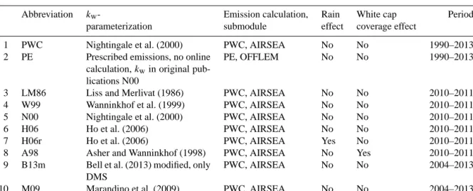
Table 1. Set-up of model simulations evaluated in this study. PWC: prescribed water concentration, PE: prescribed emissions, AIRSEA:

submodel for online calculation of emissions, OFFLEM: submodel for prescribing emissions.

Abbreviation k_w- Emission calculation, Rain White cap Period

parameterization submodule effect coverage effect

1 PWC Nightingale et al. (2000) PWC, AIRSEA No No 1990–2013

2 PE Prescribed emissions, no online calculation,kwin original publications N00

PE, OFFLEM No No 1990–2013

3 LM86 Liss and Merlivat (1986) PWC, AIRSEA No No 2010–2011

4 W99 Wanninkhof et al. (1999) PWC, AIRSEA No No 2010–2011

5 N00 Nightingale et al. (2000) PWC, AIRSEA No No 2010–2011

6 H06 Ho et al. (2006) PWC, AIRSEA No No 2010–2011

7 H06r Ho et al. (2006) PWC, AIRSEA Yes No 2010–2011

8 A98 Asher and Wanninkhof (1998) PWC, AIRSEA No Yes 2010–2011

9 B13m Bell et al. (2013) modified, only DMS

PWC, AIRSEA No No 2004–2013

10 M09 Marandino et al. (2009) PWC, AIRSEA No No 2004–2013

scribed in Z13 and L11 (1^◦×1^◦in both). It has to be noted that this leads to a smoothing of small, local hotspots, but we assume this to be negligible since we compare emissions on a global scale.

Besides the concentrations taken from the climatologies Z13/L11, the air–sea calculation requires information on sea surface temperature, salinity and wind. The mean sea surface temperature in the model for simulation 1 (1990–2013) was 15.95^◦C, 15.82^◦C in Z13 and 16.22^◦C in L11. The mean wind speed in the EMAC simulations (PWC, PE) was

7.51 m s⁻¹, which is slightly larger than the wind speed used to calculate the emission climatologies in Z13 (EMAC is 4.7 % larger) and L11 (EMAC is 2.7 % larger). Sea surface salinity is prescribed with a constant value of 0.4 mol L⁻¹in our model simulations as opposed to spatially varying salinity in Z13 and L11. A 2-year simulation comparing the effects of a constant salinity versus the Z13 climatology revealed a low effect on global emissions (<3 %), which is in accordance with findings of Ziska et al. (2013). Compared to the calculation of the Schmidt number in the publications by

(6)

Z13 and L11, the submodel AIRSEA uses a different empiri- cal, temperature-dependent equation to calculate the Schmidt number. In AIRSEA, the Schmidt number of CO₂at the respective temperature is calculated and then adapted with the molar volume to the Schmidt number of the gas of interest (Wilke and Chang, 1955; Hayduk and Laudie, 1974). In Z13, the Schmidt number is calculated by averaging the diffusion coefficient according to Hayduk and Laudie (1974) and Wilke and Chang (1955) and then dividing by the dynamic viscosity of seawater at varying temperatures and a constant salinity of 35. In L11, the Schmidt number is calculated according to Saltzman et al. (1993). The resulting differences are negligible at sea surface temperatures higher than 10^◦C and grow largest at 0^◦C, where they are still less than 15 %.

Since the Schmidt number is then normalized to the Schmidt number of CO₂, the resulting difference becomes small and does not lead to significant differences in the global emission estimates of all four compounds. Differences in other influential input parameters for emission calculation between our PWC set-up and Z13 and L11 are thus small, ensuring that differences in emissions between PWC and Z13 and L11 can be attributed to the consideration of the actual state of the atmosphere in the PWC set-up.

2.3.2 Transfer velocity parameterizations

In the second part of the study, we test the sensitivity of the global emissions towards eight different transfer velocity parameterizations. These tests cover a 2-year time span (2010–

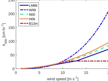
2011) with 1 year (2009) as spin-up. The simulations 3–6 (Table 1) test the impact of different water-side transfer velocity parameterizations related to wind speed. The parameterizations tested in this study are illustrated in Fig. 2. With increasing wind speed, the differences between the transfer velocity parameterizations grow larger; hence, testing these parameterizations yields a range of global emission estimates that reflects this uncertainty. Parameterizations and the general description of air–sea gas exchange calculation are described in Sect. 2.2.

Table 1 provides an overview of all performed simulations.

Simulation 3 uses the 3-step linear parameterization of Liss and Merlivat (1986, LM86), simulation 4 the cubic relationship by Wanninkhof and McGillis (1999, W99), simulation 5 the quadratic parameterization by Nightingale et al. (2000, N00), and simulation 6 the quadratic transfer velocity parameterization by Ho et al. (2006, H06). The effect of rain (simulation 7 in Table 1) was tested adding the Ho et al. (1997) rain effect parameterization to the H06 transfer velocity parameterization (see Pozzer et al., 2006, Eqs. 10 and 11). White cap coverage according to Asher and Wanninkhof (1998, A98) considers bubble-mediated gas exchange and is used in simulation 8. The different parameterizations (LM86, W99, N00, H06) were available from the AIRSEA version of Pozzer et al. (2006). The N00 parameterization was normalized to

wind speed [m s^-1]

0 5 10 15 20

k660 [cm hr-1 ]

0 50 100 150 200 250

LM86 W99 N00 H06 B13m

Figure 2. Parameterizations for water-side transfer velocity of air–

sea gas exchangekwfor a Schmidt number of 660 that are tested in this study: the linear parameterization LM96 (Liss and Merlivat, 1986), the cubic parameterization W99 (Wanninkhof and McGillis, 1999), the quadratic parameterization N00 (Nightingale et al., 2000) and H06 (Ho et al., 2006), the parameterization modified according to Bell et al. (2013, B13m) with a levelling off at wind speeds higher than 11 m s⁻¹, and the linear parameterization M09 (Marandino et al., 2009).

the Schmidt number of 600 as in the original publication by Nightingale et al. (2000), while 660 was used in Z13.

Two additional simulations including only DMS were performed to test the effect of two recently published parameterizations ofk_w. These two parameterizations have been derived from in situ DMS eddy covariance measurements and deviate from previously published parameterizations. Bell et al. (2003) observed that the transfer velocity does not increase at wind speeds higher than 11 m s⁻¹. Marandino et al. (2009) found a linear dependency between wind speed and the transfer velocitykwfor DMS. Both simulations cover the period of 2004–2013, since observations from this period were available for comparison. These two parameterizations forkw were added to the submodule code of AIRSEA (for equations see Table 4). The modification of the code included a parameterization based on results of the study from Bell et al. (2013, B13m) with a conservative approach, in which the N00 parameterization was used at wind speeds below 11 m s⁻¹and kept constant at higher wind speeds to account for the missing increase ofk_wwith increasing wind speed. Fi- nally, the parameterization by Marandino et al. (2009, M09) was used in simulation 10 for the same period as B13m. Both newly implemented parameterizations are part of the most recent release MESSy 2.52.

2.4 Observational data

Simulated atmospheric mixing ratios of the trace gases from PWC and PE are compared to observations from ship cam-

(7)

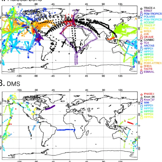
Figure 3. Locations of atmospheric data for comparison with model output used in this study. Panel (a) shows locations of atmospheric measurements from 23 aircraft campaigns considered for comparison with halocarbon simulations. Panel (b) shows location of measurements in the atmospheric boundary layer from ships (PHASE-1, Knorr-06, Knorr-07, M98) and from aircraft campaign (HIPPO 1–5) measurements considered for comparison with DMS simulations.

paigns, aircraft campaigns and ground-based time series stations.

A total of 23 aircraft campaigns providing halocarbon data are considered in order to create annual zonal mean climatologies of these trace gases. The combined data set ranges from 90^◦N to 75^◦S, transecting from the surface to the upper troposphere/lower stratosphere over land and ocean from 1992 to 2012 (see Table S1 for details on the aircraft campaigns). Many of the more recent data sets are inter- calibrated (see e.g. Brinckmann et al., 2012; Hall et al., 2014;

Sala et al., 2014; Wisher et al., 2014). The latitudinal and lon- gitudinal distributions and names of the aircraft campaigns are illustrated in Fig. 3a. The measurements were averaged in zonal 10^◦wide latitude bins with a vertical extent ranging from 10 to 50 hPa (10 hPa in boundary layer and TTL regions). Most of the measurements are located around 30^◦N of latitude with more than 150 points per bin. The tropical

region (20^◦N–20^◦S) has an average of 50 points per bin.

Figure S1 in the Supplement illustrates the numbers of the measurements per bin. For the comparison of measured and modelled data, the EMAC output of simulations 1 and 2 is first sampled at the same location as the aircraft measurements (longitude, latitude, altitude and time) by linear inter- polation. Then, the same process of averaging per bin as for the measurements is applied to the model output.

Nine coastal ground stations from NOAA/ESRL, where halocarbons have been measured by the NOAA global flask sampling network starting from 1990–2004 were chosen for comparison due to their location close to the coast (Table 2).

These data are currently available at the HalOcAt (Halocar- bons in the Ocean and Atmosphere) database (https://halocat.

geomar.de/). Two time series stations situated distant to the coast (Park Falls, Wisconsin, Niwot Ridge Forest, Colorado, both USA) were chosen to assess to contribution of marine

(8)

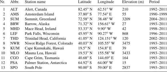
Table 2. Metadata of the ground-based time series stations of halocarbons (NOAA) considered in this study. For DMS, the data from time series of Cape Grim and Amsterdam Island were considered.

Nr. Abbr. Station name Latitude Longitude Elevation (m) Period

1 ALT Alert, Canada 82.45^◦N 62.51^◦W 210 1992–2011

2 AMS Amsterdam Island 37.80^◦S 77.54^◦E 55 1990–1999

3 SUM Summit, Greenland 72.58^◦N 38.48^◦W 3209 2004–2011

4 BRW Barrow, Alaska 71.32^◦N 156.61^◦W 27 1993–2011

5 MHD Mace Head, Ireland 53.33^◦N 9.90^◦W 42 1998–2011

6 LEF Park Falls, Wisconsin 45.95^◦N 90.27^◦W 868 1996–2011

7 THD Trinidad Head, California 41.05^◦N 124.151^◦W 120 2002–2011 8 NWR Niwot Ridge Forest, Colorado 40.03^◦N 105.55^◦W 3475 1993–2011

9 KUM Cape Kumukahi, Hawaii 19.5^◦N 154.8^◦E 39 1995–2011

10 MLO Mauna Loa, Hawaii 19.53^◦N 155.58^◦W 3433 1993–2011

11 CGO Cape Grim, Tasmania 40.68^◦S 144.69^◦E 164 1993–2011

12 PSA Palmer Station, Antarctica 64.92^◦S 64.00^◦W 15 1997–2011

13 SPO South Pole 90.00^◦S 59.00^◦E 2837 1993–2011

halocarbon emissions to the atmospheric mixing ratio over land. Monthly means of the time series were compared to monthly means of simulations 1 and 2 for the PWC and PE set-up.

DMS was directly compared to measurements from ship campaigns in the marine boundary layer, because only few data from ground-based time series stations is available. The campaigns chosen were PHASE-I (2004, Marandino et al., 2007), two campaigns on RV Knorr (Marandino et al., 2007, 2008), and M98 on RV Meteor (2009, A. C. Zavarsky, per- sonal communication, 2014) to ensure a broad spatial coverage (Fig. 3b). Additionally, DMS data from two time series stations – Cape Grim, Australia, 1990–1993 (Ayers et al., 1995) and Amsterdam Island in the Indian Ocean, 1990–

1999 (Sciare et al., 2000) – were used for comparison (Ta- ble 2). Upper air atmospheric concentrations of DMS were compared to aircraft measurements from the HIAPER Pole- to-Pole observation (HIPPO) campaigns 1–5 (Wofsy et al., 2012), again subsampling the model output for time and location of the observations.

3 Results and discussion

3.1 Global emissions based on prescribed concentrations

The long-term mean of global emissions (1990–2013, simulation 1 in Table 1) based on PWC is different from the offline calculated emission climatologies for all four gases.

The magnitude of this difference varies between the gases +11 % (CHBr3) to−28 % (CH₂Br₂)(Table 3). The global spatial pattern of the PWC emissions is similar to the spatial patterns in Z13 and L11 (Figs. 4, 5). Although global emissions for CH₂Br₂were reduced in the PWC set-up compared to the Z13 scenario, they still lie in the range of previously published estimates (61.8–112.7 Tg yr⁻¹; Table 3).

The global PWC emissions for CHBr₃are 11 % higher than from Z13, but still 47–60 % lower than top-down approaches by Warwick et al. (2006), Liang et al. (2010) and Ordóñez et al. (2012). The PWC CHBr3 emissions lie at the lower end of emission scenarios, closest to Z13. The same holds for CH3I, where emissions are 2 % higher compared to Z13 but still 18 % lower than the published estimate from Bell et al. (2002). Emission estimates in PWC are closest to Z13 and thus at the lower end of the range of published global emission estimates. DMS emissions in PWC compared to L11 were 17 % lower (Table 3).

The main differences between PE and PWC result from considering the actual state of the atmosphere when calculating emissions from PWC, since the atmospheric mixing ratio of the gas has a direct feedback on its emissions through the concentration gradient (Eq. 1). Higher atmospheric concentrations lead to lower marine emissions (or can even lead to deposition) and vice versa. In the PWC set-up where the actual concentration gradient between the ocean surface concentration and the model’s atmospheric mixing ratio is considered, the emissions thus respond consistently to this feedback. The most obvious example for that is the global emission of DMS. In L11, an atmospheric concentration of 0 ppt is assumed justified by the high supersaturation in the water and the short lifetime of DMS. In the PWC approach in our study, the atmospheric mixing ratio is always higher than 0 ppt, on average 133 (±125) ppt, and this is likely the main reason for the resulting 17 % reduction in the modelled flux vs. L11 (Fig. 5).

Considering the actual state of the atmosphere leads to al- tered concentration gradients and thus emissions for any gas in the PWC set-up, but the impact on global emissions depends on the specific characteristics and global distribution of the gas in the surface ocean. For example, the impact of the PWC approach on global emissions for CH2Br2 (28 % difference between PWC and Z13) is larger than that for CH3I

(9)

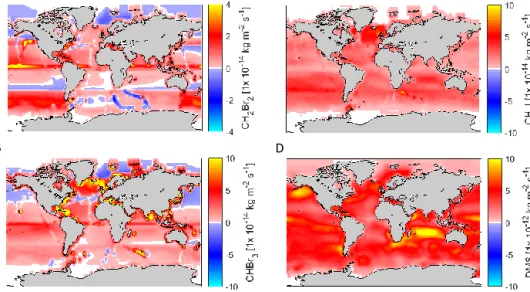
A C

B D

Figure 4. Emissions from PWC (N00 parameterization forkw)for the trace gases dibromomethane (CH₂Br₂, panel a), bromoform (CHBr₃, panel b), methyliodide (CH₃I, panel c) and dimethyl sulfide (DMS, panel d), their annual mean of the period 1990–2013 (simulation 1, Table 1).

(2 % difference) (Table 3). This difference can be explained by the saturation of the two gases: CH₃I is mainly oversat- urated in the surface ocean with a mean saturation ratio (actual concentration divided by equilibrium concentration) of 18.2 in Z13. CH2Br2 with a mean saturation ratio of 2 is concentrated closer to equilibrium. The distance from equilibrium is thus larger for CH3I than for CH2Br2. Changes in atmospheric mixing ratio therefore affect the concentration gradient for CH2Br2more than for CH3I. For CHBr3with a similar global ocean surface saturation ratio as CH₂Br₂, a drastic change in emissions between PWC and Z13 can be seen in the Southern Hemisphere (50–90^◦S; Table 3), where the emissions increase 2 orders of magnitude in the PWC compared to Z13. The Z13 emission climatology displays a latitudinal band of elevated atmospheric mixing ratios around 60^◦S, which result in this region being a sink for atmospheric CHBr₃. In our PWC set-up, atmospheric mixing ratios in this region are not as elevated and hence PWC leads to larger emissions. In general, gases that are concentrated close to equilibrium in the surface ocean respond more strongly to changes in atmospheric concentrations and thus to the PWC set-up than more supersaturated gases.

Comparing integrated regional fluxes, the halocarbons dis- play the largest differences in the polar regions (Table 3).

Besides dynamic atmospheric concentrations that may alter emissions in the PE set-up, two other reasons for differences in this specific set-up apply for the halocarbons. First, no sea ice is considered in Z13 whereas EMAC uses prescribed sea ice in our PWC set-up. L11 considers sea-ice. When sea ice is present in the model EMAC/AIRSEA, the flux is reduced by the fraction of surface that is covered by it. This may lead to the lower flux estimations in our PWC set-up and may partly

explain e.g. the reduced emissions in the Arctic for CHBr₃. Furthermore, our PWC approach takes into account air-side transfer velocity (Eq. 2) instead of only the water-side transfer velocity as Z13, which can control the flux of more soluble gases at low temperatures and thus decrease emissions (McGillis et al., 2000). At high latitudes (60–90^◦N and S), where low temperatures and high winds prevail, the transfer velocity can be reduced by up to 68 % (CH2Br2), 32 % (CHBr3)and 61 % (CH3I) usingkairin the PWC set-up. L11 takes thekairand sea ice into account, so this difference does not apply.

3.2 Atmospheric mixing ratios based on PWC and PE The atmospheric mixing ratios in EMAC sustained by emissions either from PWC or PE are compared to available atmospheric observations from aircraft campaigns (halocarbons, DMS), ground-based time series stations from NOAA/ESRL (halocarbons) and ship campaigns (DMS). The model output of simulations 1 and 2 (Tables 1, 4) was subsampled at the times and locations of the observations. A scatterplot for direct comparison between model output and observations is provided in the Supplement in Fig. S2.

The largest difference between PWC and PE in the atmospheric mixing ratio is again found for CH₂Br₂ in the Southern Hemisphere (Fig. 6), where the PWC set-up yields lower emissions and therefore also lower atmospheric mixing ratios. For CH₂Br₂, atmospheric mixing ratios globally decrease on average by 28 % compared to the PE set-up, which is the same percentage as the reduction in the global emissions. Concentrations derived from these reduced fluxes gen- erally agree better with the measurements, even though Arc- tic emissions still seem to be underestimated in the model

(10)

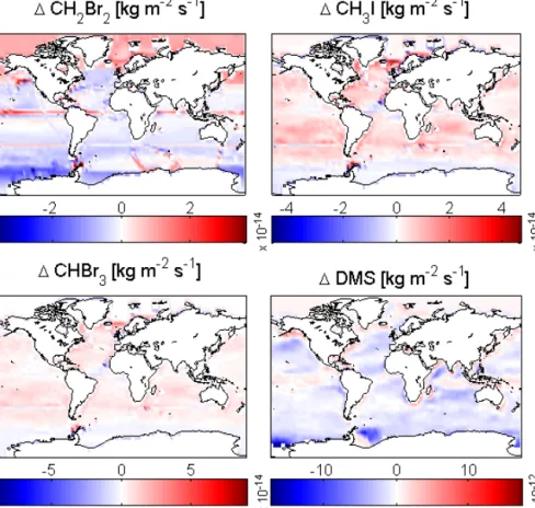
Figure 5. Differences (PWC–PE) in emissions between PWC (simulation 1, Table 1, 2010–2011) and PE (simulation 2, Table 1, 2010–2011).

Red indicates a larger flux in the PWC set-up, blue a larger one in the PE set-up.

compared to the observations. A possible explanation for this underestimation could be emissions of VSLS from sea ice that are not considered in the model, as e.g. Karlsson et al. (2013) observed elevated CH2Br2in brines on top of sea ice. Mixing ratios of CHBr3 are similar in the PWC and PE set-ups (difference globally only 1.2 %), but both do not show the same pattern as the measurements: for both set-ups, atmospheric mixing ratios are underestimated in the Southern Hemisphere up to the northern tropics (Fig. 6). The same is evident for CH₃I, where PWC and PE also vary only slightly, while both set-ups underestimate atmospheric CH₃I concentration in the tropics. Since atmospheric concentrations were derived from emissions based on the Z13/L11 water concentration climatology in the PWC set-up, nega- tive discrepancies to atmospheric observations indicate regions where the concentration climatologies lack hotspots and can thus identify missing oceanic source regions. For all three halocarbons, the concentration climatologies seem to represent water concentrations that are too low in the North- ern Hemisphere and the tropics to explain the observed atmospheric mixing ratios. It has to be noted that coastal ar- eas are large source regions of halocarbon emissions with global contributions of up to 70 % (Ziska et al., 2013), which

might be underrepresented in our modelled approach and thus might at least partly explain these missing sources.

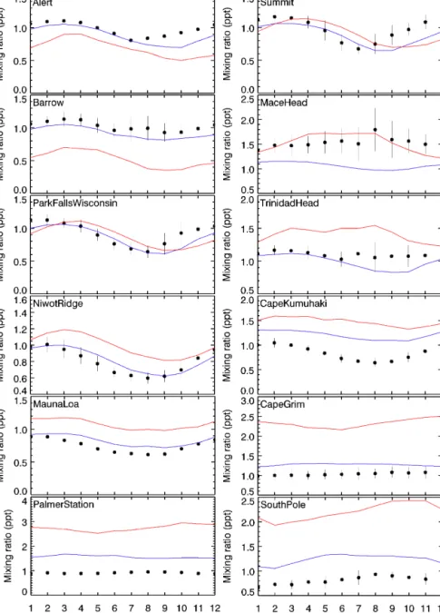
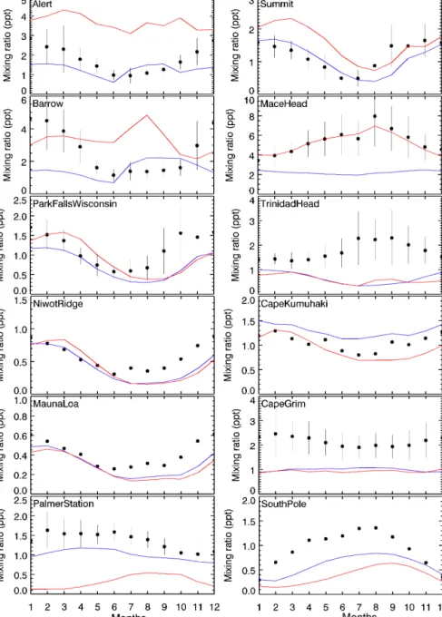
Modelled concentrations matched observations from NOAA/ESRL ground stations in most of the cases better in the PWC set-up compared to PE. The agreement between simulation and measurements increases with the atmospheric lifetime of the gases: modelled mixing ratios for CH₂Br₂, with the longest lifetime of the tested gases, reflect the observed seasonality at all 12 stations well (Fig. 7). The modelled seasonality of the atmospheric mixing ratios is similar in both the PWC and PE set-ups, indicating that the main fluctuations at these locations comes from seasonality in atmospheric transport and chemistry rather than from seasonality in emissions, since emissions are constant in PE. For all stations except for Mace Head, PWC yields atmospheric mixing ratios closer to the measurements for CH₂Br₂, re- ducing overestimations of modelled atmospheric mixing ratios compared to measurements of up to 75 % as e.g. at the South Pole. Discrepancies between observations and model simulations are larger in most of the ground-based stations for CHBr3 (lifetime ∼20 days in our simulation) than for CH₂Br₂, and again PWC yields as good or more accurate mixing ratios than PE compared to the measurements (Fig. 8). However, the observed seasonality is not well re-

(11)

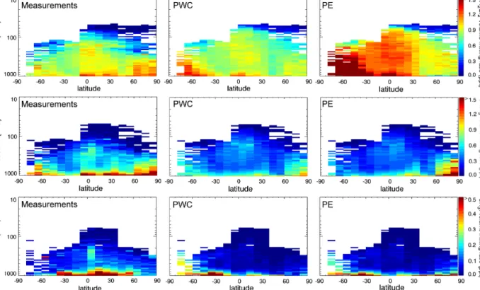
Figure 6. Atmospheric mixing ratios (in ppt) of the trace gases dibromomethane (CH₂Br₂, upper row), bromoform (CHBr₃, middle row), and methyliodide (CH₃I, lower row) derived from measurements (see Fig. 3 for locations of aircraft campaigns) and EMAC runs with prescribed water concentrations and prescribed emissions. Model output was subsampled at locations and times of observations and binned for direct comparison.

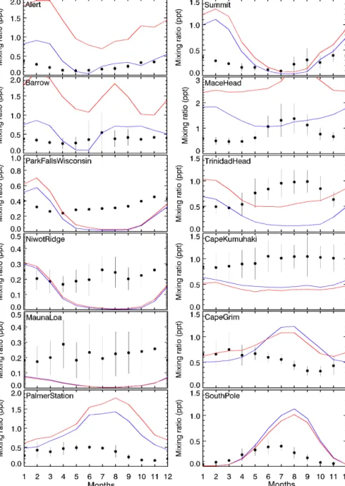
flected in either the PWC or the PE set-up. This mismatch indicates that a further seasonality in the sources is required, which can e.g. be accounted for by introducing a seasonality in the water concentrations prescribed. This finding is op- posite to findings from Liang et al. (2010), who concluded that atmospheric CHBr₃mixing ratios are mainly driven by transport and atmospheric chemistry. Furthermore, the good agreement between model and observations at continental sites away from the coast (Park Falls, Wisconsin, USA; Ni- wot Ridge Forest, Colorado, USA) for CH₂Br₂and CHBr₃ indicates that the ocean is the dominant source of these compounds also over land. CH₃I, the gas with the shortest lifetime in the range of a few days, shows the largest discrepancies between modelled mixing ratios and observations (Fig. 9). The PWC set-up yields mixing ratios in the range of the observations for only two stations (Alert, Canada, and Barrow, Alaska, USA) and, in most of the stations, the seasonality was not well reflected in the model runs. CH3I seasonality in water concentrations has previously been observed (Shi et al., 2014), indicating that seasonally resolved water concentrations are needed to reproduce atmospheric concentrations of the shortest-lived compounds in a more accurate way. Oceanic emissions in PE and PWC were too large to explain atmospheric mixing ratios at stations in high latitudes (Summit, Mace Head, Cape Grim, Palmer Station,

South Pole), but too low to explain atmospheric mixing ratios in lower latitudes (Park Falls, Trinidad Head, Niwot Ridge, Cape Kumukahi, Mauna Loa), which agrees with findings from aircraft campaigns (Fig. 6).

Four ship campaigns were chosen for comparison of DMS, since only few long-term measurements of atmospheric mixing ratios of DMS are available. Simulation with both the PWC (N00) and the PE approach overestimate DMS mixing ratios in the marine boundary layer from ship campaigns (see positive mean bias in Table 5). However, the PWC reduces discrepancies within both ship and aircraft campaigns by a factor of 2 (Table 5), as the mixing ratio is overes- timated by a factor of 0.61 in PWC as opposed to 1.31 in PE. The observed seasonality of DMS mixing ratios at Amsterdam Island is well reflected in the simulations except for the summer months, where PWC and PE overestimate the monthly mean by a factor of up to 4.6 (PWC) and 6.7 (PE) (Fig. 10). At Amsterdam Island, the simulated annual mean atmospheric mixing ratio of 180.7 ppt in the PWC set-up agrees very well with the observed annual mean of 181.2 ppt, whereas the simulated annual mean in the PE set- up is 268.5 ppt. At Cape Grim, the results of the two set-ups do not differ that much, and both simulations underestimate the mixing ratios measured during austral summer.

(12)

Figure 7. Mean seasonal variation of CH₂Br₂mixing ratios (in ppt) using model output based on PE (in red) and PWC (in blue), subsampled at the location of the NOAA ground-based time series stations. Black dots indicate the long-term monthly means of the time series at the specific locations (±standard deviation of the monthly means), vertical lines indicate the corresponding standard deviations. Monthly time series of at least 7 years were averaged, the exact periods are listed in Table 2.

An overall comparison of the agreement of both set- ups with observations is summarized in a Taylor diagram (Fig. 11). This diagram is a statistical summary that shows how well two patterns match each other with regard to their correlation, variance and root-mean-square difference (Tay- lor, 2001). The closer a point of a specific set-up is located to the reference point of observations (here 1.0 onx axis), the more the simulation resembles the observed measurements.

PWC simulations increased the agreement with observations for CH2Br2, especially the correlation (0.4 in PE to 0.6 in

PWC), and for DMS (0.53 in PE to 0.65 in PWC), but only very slightly for CHBr₃and CH₃I. Centred statistics for all compounds can be found in Table 5, with the equations used to compute the statistics according to Yu et al. (2006) listed in the Supplement.

3.3 Comparison of different transfer velocity (k_w) parameterizations

A large uncertainty of global emission estimates is related to different parameterizations of the transfer velocity in Eq. (1).

(13)

Figure 8. Same as Fig. 7, for CHBr₃.

Calculating emissions online enables a simple way of testing different transfer velocity parameterizations, which was real- ized here with eight 2-year simulations described in Table 1 (simulations 3–10).

The largest sensitivity for the emissions of all gases is introduced by different parameterizations of the water-side transfer velocitykwtested in simulations 3–6 (Table 4). The 4 parameterizations that were tested (simulation 3–6, Ta- ble 1) comprised linear (LM86, simulation 3), cubic (W99, simulation 4) and quadratic (N00, simulation 5, H06, simulation 6) relations to wind speed. The resulting global emission estimates in these parameterizations range 53.7–

65.1 Gg yr⁻¹ for CH₂Br₂, 189.0–249.7 Gg yr⁻¹for CHBr₃,

151.9–225.7 Gg yr⁻¹ for CH3I and 33.4–48.7 Tg yr⁻¹ for DMS (Table 4). As expected, the linearkwparameterization (LM86) yields the lowest global emission estimates, since it produces the lowestkw values (Fig. 2). The N00 parameterization produces the highest global fluxes for CHBr3and CH₂Br₂but not for DMS and CH₃I, where the highest fluxes were obtained by H06 (DMS) and W99 (CH₃I) (Table 4).

The fact that different parameterizations lead to higher global estimates for different gases is explained by the varying spatial distribution of concentration hot spots and regional variations of wind.

Thek_wparameterization in simulation 7 increases the flux under calm conditions due to precipitation. This increase

(14)

Figure 9. Same as Fig. 7, for CH₃I.

ranged from 4 % (CH₂Br₂)to 6 % (DMS) (Table 4) when compared to the reference flux using H06 alone (simulation 6, Table 4). Additional flux due to precipitation is in- versely correlated to the Schmidt number, so that under iden- tical conditions, increasing flux would be added in the order CHBr₃>CH₂Br₂>DMS >CH₃I. The global flux estimations compared to the reference run do not increase in this order (Table 4), rather DMS> CHBr₃∼CH₃I>CH₂Br₂. This non-uniform response among the gases is explained by the globally and regionally varying distance from equilibrium for the four gases, which together with regional precipitation patterns leads to variations in the emissions increased by rain. The parameterization based on white-cap coverage

(A98) also has small but ambivalent effects on the global flux for the different compounds (simulation 8, Table 4). Com- pared to the mean of all nonlinear parameterizations for each gas, global emissions were higher when the white cap coverage parameterization was used for CHBr₃(4 %) and CH₂Br₂ (2 %) but lower for CH₃I (−8 %) and DMS (−6 %) (Table 4).

The parameterizations tested only for DMS are both derived from eddy covariance measurements at sea. Both parameterizations changed the global emissions by −4.4 % (B13m) and −1.2 % (M09) compared to the average flux of simulations 3–6 (Table 4). Although the modelled atmospheric mixing ratios at the time and location of observations is for both of the parameterizations higher than the observa-

(15)

Table3.Integratedglobalfluxesfromthisstudy(PWC:prescribedwaterconcentrations,N00:kwparameterizationofNightingaleetal.,2000)comparedtopreviouslypublished emissionestimates.NotethatZiskaetal.(2013)isabottom-upapproachandthewaterconcentrationswereusedintheonlinefluxcalculationsforthehalocarbons;Lanaetal.(2011) DMSwaterconcentrationswereusedforDMSonlinecalculations.Ordóñezetal.(2012),Liangetal.(2010),andWarwicketal.(2006)aretop-downapproaches,Belletal.(2002)is anoceanicmixed-layerbottom-upmodelapproachforCH3I. CH2Br2(Ggyr−1)CHBr3(Ggyr−1)CH3I(Ggyr−1)DMS(Tgyr−1) ThisstudyZiskaetal.Ordóñezetal.Liangetal.Warwicketal.ThisstudyZiskaetal.Ordóñezetal.Liangetal.Warwicketal.ThisstudyZiskaetal.Belletal.ThisstudyLanaetal. (PWC,N00)(2013)(2012)(2010)(2006)(PWC,N00)(2013)(2012)(2010)(2006)(PWC,N00)(2013)(2002)(PWC,N00)(2011) 90–50◦N1.3−4.01.61.30.326.744.813.39.40.913.420.314.02.12.3 50–20◦N12.516.515.314.910.549.033.9123.2108.127.936.840.589.97.28.5 20◦N–20◦S32.238.441.134.384.5108.594.1286.9249.0517.463.359.391.218.021.1 20–50◦S7.819.37.79.716.541.442.098.070.543.880.767.782.413.916.5 50–90◦S9.117.20.91.60.912.80.17.011.62.415.517.014.94.26.0 Total63.087.466.661.8112.7238.4214.9528.4448.6592.4209.7204.8291.745.554.4

A

B

Amsterdam Island

Cape Grim

Figure 10. Same as Fig. 7, for DMS.

Standard deviation

0.0 0.5 1.0 1.5 2.0 2.5

0.00.51.01.52.02.5

1 2

● 0.1 0.2

0.3 0.4

0.5 0.6

0.7

0.8

0.9

0.95

0.99 Correlation

●

●●

●

CH2Br2 PE CH2Br2 PWC CHBr3 PE CHBr3 PWC CH3I PE CH3I PWC DMS PE DMS PWC

Figure 11. Taylor diagram of PE (triangles) compared to PWC (cir- cles) runs using the same parameterization fork_w(N00) for comparison. The Taylor diagram relates model simulations to observations according to their root-mean-square error (given as the distance to the reference point,xaxis 1.0), correlation and standard deviation.

Simulations located closest to the reference point agree best with observations.

(16)

Table 4. Integrated global emissions during 2010–2011 for sensitivity tests using different parameterizations for the transfer velocitykw (simulations 3–6, same as in Table 1) and the effects of rain (simulation 7), bubble-mediated transfer parameterized using white cap coverage (simulation 8) and parameterizations recently suggested for DMS (simulations 9 and 10). Equations for the parameterizations using wind speeduare given for the Schmidt number (subscript afterk) as in the original publications listed.u: wind speed at 10 m a.s.l. in metres per second.kis given in centimetres per hour.

No. Parameterization CH₂Br₂ CHBr₃ CH₃I DMS

Gg yr⁻¹ Gg yr⁻¹ Gg yr⁻¹ Tg yr⁻¹ 3 Liss and Merlivat (1986) foru≤3.6,k₆₆₀=0.17u

for 3.6< u <13,k₆₆₀=2.85u−9.65 foru≥13,k₆₆₀=5.9u

53.74 189.10 151.88 33.38

4 Wanninkhof et al. (1999) k₆₆₀=0.0283u³ 58.38 211.17 223.52 45.22

5 Nightingale et al. (2000) k₆₀₀=0.22u²+0.333u 63.04 238.46 209.73 45.49

6 Ho et al. (2006) k₆₆₀=0.266u² 62.71 236.10 213.47 45.91

7 Ho et al. (2006)+rain – 65.08 249.66 225.67 48.70

8 White cap coverage – 62.76 238.51 197.44 42.53

9 Bell et al. (2013), modified foru≤11,k₆₀₀=0.22u²+0.333u foru >11,k₆₀₀=30.283

– – – 40.63

10 Marandino et al. (2009) k₇₂₀=1.92u−1.0^∗ – – – 42.45

Mean (simulations 3–6) 59.47 218.71 199.65 42.5

* Units converted, in original publication:k₇₂₀=0.46u−0.24 (m day⁻¹).

Table 5. Error metrics for the comparison of model output from PWC (simulation 1) and PE (simulation 2) for all of the compounds including all aircraft campaigns and ship observations, illustrated in Fig. S2 in the Supplement. Determination of error metrics according to Yu et al. (2006).

CH₂Br₂PE CH₂Br₂PWC CHBr₃PE CHBr₃PWC CH₃I PE CH₃I PWC DMS PE DMS PWC

Mean bias (ppt) 0.24 −0.036 −0.23 −0.24 −0.14 −0.14 86.21 42.12

Mean absolute gross error (ppt) 0.30 0.15 0.31 0.31 0.15 0.16 102.9 67.39

RMSE (ppt) 0.381 0.21 0.53 0.53 0.26 0.26 236.2 135.8

Fractional bias (ppt) 0.26 0.0001 −0.23 −0.20 −0.89 −0.96 0.23 0.10

Fractional absolute error (ppt) 0.31 0.20 0.56 0.56 1.13 1.19 1.23 1.18

Normalized mean bias factor (–) 0.27 −0.04 −0.49 −0.53 −1.71 −1.96 1.31 0.64

tions, discrepancies between simulated and observed mixing ratios were reduced compared to the N00 parameterization by factors of 1.4 (B13m) and 1.2 (M09).

4 Summary and conclusions

Two different ways of considering marine emissions of trace gases in global atmospheric chemistry models are discussed here for the halocarbons CH2Br2, CHBr3, CH3I and the sulfur-containing compound DMS. In contrast to prescribing emissions (PE) from oceanic and atmospheric concentration climatologies in the model, prescribing water concentrations (PWC) with an online calculation of emissions results in a consistent concentration gradient between ocean and atmosphere. The approach of modelling emissions online was suc- cessfully applied for the very short-lived halocarbons for the first time. The approach is based on the submodel AIRSEA coupled to EMAC by Pozzer et al. (2006). The method has a number of conceptual and practical advantages, as in this framework the modelled flux can respond in a consistent way

to changes in sea surface temperature, surface wind speed, possible sea ice cover and marine atmospheric mixing ratios in the model.

Global emission estimates of the four gases differ between +11 % (CHBr₃)and−28 % (CH₂Br₂)between PWC and PE when the transfer velocityk_wis parameterized according to Nightingale et al. (2000) in both set-ups. Prescribing water concentrations instead of emissions has the strongest effect for gases close to equilibrium in the surface ocean such as CH2Br2(28 % reduced emissions in PWC compared to PE), as its emissions are most sensitive to atmospheric concentrations. In contrast, only a 2 % difference is found for the highly supersaturated gas CH₃I. Considering PWC reduces the global emissions of DMS by 17 %, a comparison to observations revealed that PWC compared to PE reproduces observations slightly (CHBr₃, CH₃I) or much (CH₂Br₂, DMS) better for measurements made at ground-based time series stations, aircraft campaigns and ship cruises. Even though it is clear that more data for all compounds are needed globally, the PWC set-up can be used to identify oceanic regions