Mixtures of t-distributions for Finance and Forecasting

IHS Economics Series Working Paper 216

October 2007

Mixtures of t-distributions for Finance and Forecasting

Raffaella Giacomini

Impressum Author(s):

Raffaella Giacomini, Andreas Gottschling, Christian Haefke, Halbert White Title:

Mixtures of t-distributions for Finance and Forecasting ISSN: Unspecified

2007 Institut für Höhere Studien - Institute for Advanced Studies (IHS) Josefstädter Straße 39, A-1080 Wien

E-Mail: o ce@ihs.ac.atffi Web: ww w .ihs.ac. a t

All IHS Working Papers are available online: http://irihs. ihs. ac.at/view/ihs_series/

This paper is available for download without charge at:

https://irihs.ihs.ac.at/id/eprint/1800/

216 Reihe Ökonomie Economics Series

Mixtures of t-distributions for

Finance and Forecasting

216 Reihe Ökonomie Economics Series

Mixtures of t-distributions for Finance and Forecasting

Raffaella Giacomini, Andreas Gottschling, Christian Haefke, Halbert White

October 2007

Contact:

Raffaella Giacomini University College London email: r.giacomini@ucl.ac.uk Andreas Gottschling Deutsche Bank AG Credit RiskManagement

email: andreas.gottschling@db.com Christian Haefke

Department of Economics and Finance Institute for Advanced Studies, Vienna email: haefke@ihs.ac.at

Halbert White

Department of Economics University of California, San Diego email: hwhite@ucsd.edu

Founded in 1963 by two prominent Austrians living in exile – the sociologist Paul F. Lazarsfeld and the economist Oskar Morgenstern – with the financial support from the Ford Foundation, the Austrian Federal Ministry of Education and the City of Vienna, the Institute for Advanced Studies (IHS) is the first institution for postgraduate education and research in economics and the social sciences in Austria.

The Economics Series presents research done at the Department of Economics and Finance and aims to share “work in progress” in a timely way before formal publication. As usual, authors bear full responsibility for the content of their contributions.

Das Institut für Höhere Studien (IHS) wurde im Jahr 1963 von zwei prominenten Exilösterreichern – dem Soziologen Paul F. Lazarsfeld und dem Ökonomen Oskar Morgenstern – mit Hilfe der Ford- Stiftung, des Österreichischen Bundesministeriums für Unterricht und der Stadt Wien gegründet und ist somit die erste nachuniversitäre Lehr- und Forschungsstätte für die Sozial- und Wirtschafts- wissenschaften in Österreich. Die Reihe Ökonomie bietet Einblick in die Forschungsarbeit der Abteilung für Ökonomie und Finanzwirtschaft und verfolgt das Ziel, abteilungsinterne Diskussionsbeiträge einer breiteren fachinternen Öffentlichkeit zugänglich zu machen. Die inhaltliche Verantwortung für die veröffentlichten Beiträge liegt bei den Autoren und Autorinnen.

Abstract

We explore convenient analytic properties of distributions constructed as mixtures of scaled and shifted t-distributions. A feature that makes this family particularly desirable for econometric applications is that it possesses closed-form expressions for its anti-derivatives (e.g., the cumulative density function). We illustrate the usefulness of these distributions in two applications. In the first application, we use a scaled and shifted t-distribution to produce density forecasts of U.S. inflation and show that these forecasts are more accurate, out-of- sample, than density forecasts obtained using normal or standard t-distributions. In the second application, we replicate the option-pricing exercise of Abadir and Rockinger (2003) using a mixture of scaled and shifted t-distributions and obtain comparably good results, while gaining analytical tractability.

Keywords

ARMA-GARCH models, neural networks, nonparametric density estimation, forecast

accuracy, option pricing, risk neutral density

Comments

The authors wish to thank Karim Abadir, John Bilson, Manfred Deistler, Carl FitzGerald, Jens Jackwerth, Eugene Kandel, Christian Krattenthaler, Andrew Patton, Michael Rockinger, Michael Wolf, and participants of the European Summer Symposium in Financial Markets in Gerzensee for helpful discussions and valuable suggestions. Two anonymous referees and an associate editor provided helpful suggestions that substantially improved this paper. Haefke acknowledges financial support from EU grant HPMF-CT-2001-01252. Part of this paper was written while Haefke was visiting UCLA. He thanks the department of economics for its hospitality. White’s participation was supported by NSF grants SBR 9811562 and SES 0111238.

Contents

1 Introduction 1

2 A Flexible Family of Density Functions 2 3 Mixture Distributions and Artificial Neural Networks 4 4 An Application to Inflation Density Forecasting 7

4.1 Generating time-varying density forecasts ... 7

4.2 Estimation and out-of-sample evaluation ... 8

4.3 Results ... 10

4.3.1 Model 1: Normal disturbances ... 10

4.3.2 Model 2: Student’s t disturbances ... 12

4.3.3 Model 3: Scaled and shifted t disturbances ... 13

5 An Application to Option Pricing 13

6 Conclusion 17 Appendix A: Proofs 18 Appendix B: Data Description 21

Appendix C: Figures 22

1 Introduction

Integrals of particular functions play a central role in economics, econometrics, and finance. For example, the price of a European call option can be expressed in terms of an integral of the cumulative distribution function (cdf) of risk neutralized asset returns. As another example, the notion of Value at Risk used to assess portfolio risk exposure is defined in terms of an integral of the probability density function (pdf) of portfolio returns. In duration analysis, unobserved variables are integrated out to avoid spurious duration dependence. For reasons of familiarity and theoreti- cal convenience, the normal distribution (or distributions derived from the normal, such as the log-normal) plays a central role in such analyses. Nevertheless, the normal distribution does not provide an empirically plausible basis for describing asset or portfolio returns, nor is it analytically tractable; neither the normal proba- bility density nor the normal cdf have closed form integrals.

This paper calls attention to the very convenient properties of Student’s t-distribution in yielding closed form

¹

expressions for the cdf and its integrals for particular sub- sets of parameter values. Even when the expressions for these integrals are not in closed form, they are still analytically quite convenient. In special cases, the inverse cdf (quantile function) also has a closed form expression, which is especially con- venient for analyzing Value at Risk. Although a closed form for the t-distribution cdf has been long known (see e.g. Moran (1968, pp 326 – 328)) this convenient property and the convenient expression for the integral of the cdf that we provide have not previously been recognized for their usefulness in economic and financial applications.

Significant flexibility is achieved by considering mixtures of scaled and shifted t-distributions, which inherit all the convenient properties of the t-distribution with respect to cdf’s and their integrals. Moreover, these mixtures have the structure of a single hidden layer artificial neural network (ANN). This ANN structure en- sures that with sufficiently many terms in the mixture and under suitable regular- ity conditions, these mixtures are capable of approximating any function and its derivatives to any desired degree of accuracy. This further suggests that mixtures of t-densities may be useful as a substitute for quadrature methods in numerical integration.

Two separate empirical applications illustrate the advantages of using t-distributions

1The definition of “closed form” is not universally agreed upon. Here, by “closed form” we mean an expression containing only a finite number of symbols, and including only the operators +,-,*,/, and a small list of trigonometric functions, inverse trigonometric functions, factorial and gamma functions, and so forth.

and their mixtures to model economic and financial time series. In the first applica- tion, we use a shifted, rescaled t -distribution to produce density forecasts of U.S. in- flation and establish whether the new distribution can provide any improvements in the out-of-sample performance of density forecasts relative to the use of the nor- mal or the standard t-distributions. We evaluate the forecasts using the framework suggested by Diebold, Gunther and Tay (1998), which makes use of the antideriva- tive of the density, thus highlighting the usefulness of the t -distribution in such applications. In the second application, we use a mixture of scaled and shifted t- distributions to estimate risk-neutral densities associated with financial options. In particular, we consider the same option-pricing application as that in Abadir and Rockinger (2003), and obtain comparably good results, while gaining in analytical tractability.

The outline of the paper is as follows. Section 2 sets forth the convenient proper- ties of the t -distribution that are our focus here. Section 3 provides a brief discussion of artificial neural networks and extends the integrability results using mixtures and artificial neural networks. This has the further benefit of bringing conditional densities into our framework. Section 4 presents our application to U.S. inflation forecasts. Section 5 presents the application to option prices. Section 6 concludes.

The appendices contain mathematical details and the proofs.

2 A Flexible Family of Density Functions

Student’s (1908) t-distribution with ν degrees of freedom has the familiar density t

_ν

(x) = = Γ

^ν+1₂

√ νπΓ

^ν₂

1 + x

²

ν

−^ν+12

, (1)

where Γ( · ) is the standard gamma function. It is a standard result that for all 0 <

m < ν − 1

Z _∞

−∞

| x |

^m

t

_ν

(x)dx < ∞ and that the integer moments are given by:

Z _∞

−∞

x

^m

t

_ν

(x)dx =







0 m odd

ν

^{m2 Γ}

(

^ν−2^m

)

Γ

(

^m+12

)

Γ

(

^ν2

)

^√π

m even.

Now we consider the antiderivatives

²

of t

_ν

. For a scalar function f of x, we write the first derivative as D f =

^{d f}_dx

. The antiderivative D

⁻¹

f is such that D(D

⁻¹

f ) = f .

2In writing the antiderivatives, the “constant of integration” is here always taken to be zero. In particular applications, other values may be appropriate.

2

In giving the antiderivative of t

_ν

, we make use of the hypergeometric function

2

F

1

. This function is defined for complex a,b,c, and z as the analytic continuation in z of the hypergeometric series

2

F

₁

(a,b; c; z) = Γ(c) Γ(a)Γ(b)

∑

∞ k=0

Γ(a + k)Γ(b + k) Γ(c + k)

z

^k

k! . (2)

The series converges absolutely for | z | < 1 , as a ratio test verifies. In our applica- tions, we are interested in the hypergeometric function for any real x. For this, we make use of the transformation z =

_x2^x+ν²

which yields | z | < 1 (see e.g. equation (89) in Abadir (1999)). Additional useful background can be found in Bailey (1962) and Slater (1966). More recently, Abadir (1999) has carefully summarized several re- sults about hypergeometric functions relevant for econometricians and economists.

Analogous to Amos (1964, Eqn. 15) we obtain the cdf of t

_ν

in closed form making use of the hypergeometric function

2

F

₁

:

Proposition 1 Let t

_ν,σ

be a scale-generalized version of (1) such that t

_ν,σ

(x), = 1

κ

_ν,σ

1 + x

²

σ

²

ν

−^ν+12

, (3)

where κ

_ν,σ

denotes the normalization factor:

κ

_ν,σ

=

Z _∞

−∞

1 + x

²

σ

²

ν

₋^ν+1₂

dx = σ √ νπ Γ

^ν₂

Γ

^ν+1₂

. (4)

Then for all x ∈ R, σ > 0, and 1 < ν < ∞:

D

⁻¹

t

_ν

(x) = 1

2 + x

κ

_ν,σ

q

(1 +

_σ^x2²ν

) ·

2

F

₁

1

2 ,1 − ν 2 ; 3

2 ; x

²

x

²

+ σ

²

ν

. (5)

₂

For nonnegative integers n such that n = ν

2 − 1 (6)

the infinite sum in

2

F

1

terminates after n terms.

The second antiderivative, D

⁻²

t

_ν

, is also of interest. For example, the price of a European call option with strike K and risk neutral cdf F ( · ) can be expressed in terms of an integral of the cumulative distribution function (cdf) of risk neutralized asset returns: C _{(K) =}

^R_K^∞

_{[1 − F (S)]} dS. The second antiderivative is given by our next result.

Theorem 1 Let t

_ν,σ

be as in 3 and κ

_ν,σ

as in Equation 4. Then for all x ∈ R, σ > 0, and 1 < ν < ∞:

D

⁻²

t

_ν,σ

(x) = x 2 + ν q

(1 +

_σ^x2²ν

) (ν − 1) κ

_ν,σ ²

F

1

− 1 2 ,1 − ν

2 ; 1 2 ; x

²

x

²

+ σ

²

ν

.

These expressions also terminate after n terms for all ν = 2(n + 1).

₂

3 Mixture Distributions and Artificial Neural Networks

Further flexibility can be achieved by considering mixtures of t-distributions, that is, by taking a convex combination of densities of scaled and shifted standard t - distributions. Just as with mixtures of normals, these mixtures can deliver skewed distributions, distributions with tail properties unachievable by a single t-distribution or distributions with two or more modes. In fact, under suitable conditions, such mixtures can approximate any distribution in large classes of probability distribu- tion functions. In addition to analytic tractability, another potential advantage of using the t-distribution instead of the normal to form a mixture is that, because of its greater flexibility, one may require fewer terms (mixing densities) in the convex combination to achieve a given accuracy of approximation to the true density.

We establish our result for mixtures of t-distributions by exploiting available results for artificial neural networks (ANNs). As we shall see next, this not only delivers results directly, but also permits us to accommodate the approximation of conditional distributions. Over the last two decades ANNs have emerged as a prominent class of flexible functional forms for function approximation. A leading case is the single hidden layer feedforward neural network, written as:

ψ (x, β,γ) = ∑

^q

j=1

β

j

· g ˜x

^T

γ

j

, (7) where ˜x = (1, x

1

,x

2

, . . . , x

r

), γ = γ

^T₁

, γ

^T₂

, . . . , γ

^T_q

T

,γ

j

∈ R

^r+1

, β = β

^T₁

, . . . , β

^T_q

T

and g : R → R is the hidden unit “activation” function. See Kuan and White (1994) for ad- ditional background.

In our discussion of desirable approximation properties, the notion of ℓ-finiteness will be useful:

Definition 1 Let ℓ be a non-negative integer. A function g is ℓ-finite if g is continu- ously differentiable of order ℓ and has Lebesgue integrable ℓ

^th

derivative.

₂

Mixtures of the form (7) are able to approximate large classes of functions (and

their derivatives) arbitrarily well, for ℓ -finite activation functions g (Hornik, Stinchcombe and White, 1990, HSW). A common choice for g is that it be a given cdf; the logistic cdf is the

leading choice. We shall pay particular attention to the case in which g is a pdf, so that its integral is a cdf. Imposing the constraint ∑

^q_j=1

β

j

= 1,β

j

≥ 0 when g is a den- sity delivers the mixture density with weights β

j

. Such mixtures can approximate arbitrary densities (White, 1996, e.g. Theorem 19.1). The form of (7) delivers not only flexibility, but it also provides the basis for analytic tractability: the properties of the integral of ψ depend solely on the properties of the integral of g .

4

Note that we view g as a univariate pdf, but that its argument is the linear combination ˜x

^T

γ

j

. For the moment, suppose that r = 1 , so ˜x

^T

γ

j

= γ

j0

+ γ

j1

· x

₁

. We therefore allow x

1

to be scaled and shifted inside g so that ψ (x,β, γ) can be viewed as a mixture of univariate pdf’s in the usual way. On the other hand, if r > 1 we can view ψ (x,β, γ) as a conditional density for one of the elements of x, say x

1

, given the rest: x

₂

, . . . , x

_r

. The use of the linear transformation ˜x

^T

γ

j

can be seen as permitting scaling and shifting as before, but with the shift now incorporating conditioning effects of the form γ

j0

+ ∑

^ri=2

x

i

γ

ji

. Thus, we view g and ψ as pdf’s for a particular random variable, though possibly conditional on other random variables. Treat- ment of multivariate densities in a framework analogous to that proposed here is possible but is beyond our present scope and is accordingly deferred.

We now turn our attention to choosing g in a way that delivers flexible closed form expressions for the integral of ψ. We do this by putting g = t

_ν

. Our next result shows that these mixtures can deliver arbitrarily accurate approximations to a large class of densities under suitable conditions.

Theorem 2 Let f belong to the Sobolev space S

_∞^m

(χ) where χ is an open, bounded subset of R

^r

. Elements of this space are functions with continuous derivatives of order m on the domain χ which satisfy

|| f ||

m,∞,χ

≡ max

n≤m

sup

x∈χ

| D

ⁿ

f (x) | < ∞ (8)

for some integer m ≥ 0 (for further background see Gallant and White (1992)). For integer ℓ < ν − 1, t

_ν

is ℓ - finite. Then for all m ≤ ℓ, f can be approximated as closely as desired in S

^m_∞

(χ) equipped with metric (8) using a single hidden layer feedforward network of the form

ψ

_ν

(x,θ) = ∑

^q

j=1

β

j

· t

_ν

x ˜

^T

γ

j

, (9)

where x ˜ = (1,x) , and q is sufficiently large.

₂

Observe that t

_ν

is always 0-finite by construction.

Corollary 1 Let T

_ν

= D

^−ei

t

_ν

denote the antiderivative of t

_ν

with respect to the i-th variable, and let l ≤ u be real numbers. Then the integral of the neural net (9) has the form

Z u

l

ψ

_ν

(x, θ)dx

i

= Ψ

_ν

(x

_(i)

(u);θ) − Ψ

_ν

(x

_(i)

(l); θ),

where x

_(i)

(a) is the vector obtained by replacing the i

^th

element x

i

from the vector x with a, and

Ψ

_ν

(x

_(i)

(a);θ) = ∑

^q

j=1

β

j

· T

_ν

(a

i j

(x

_(i)

(a), γ

i j

)),

where

a

i j

(x

_(i)

(a), γ

i j

) = aγ

i j

+

r+1

∑

k=1,k6=i

˜ x

k

γ

k j

.

Furthermore, Ψ

_ν

(x

_(i)

(a); θ) has a closed form expression (i.e. terminates after n terms) for

all ν of the form ν = 2n + 2 , n = 0, 1,2, . . . .

₂

Note that the transformed integration boundaries are different for each hidden unit because they depend on γ

i j

.

The networks Ψ

_ν

of Corollary 1 have desirable approximation properties:

Theorem 3 Let f and t

_ν

be as in Theorem 2, and let T

_ν

be as in Corollary 1. Then for integer ℓ < ν, T

_ν

is ℓ -finite and for all m ≤ ℓ , f can be approximated as closely as desired in S

^m_∞

(χ) equipped with metric (8) using a single hidden layer feedforward network of the form

Ψ

_ν

( · ) given in Corollary 1.

₂

When f is a cdf, Ψ

_ν

can approximate it, and its derivative – the associated pdf – is approximated by the derivative ψ

_ν

of Ψ

_ν

, due to the denseness in Sobolev norm and the fact that Ψ

_ν

is always 1-finite by construction.

We also have analogs of Corollary 1 and Theorem 3 for the integral of Ψ

_ν

. Corollary 2 Let Ξ

_i,ν

= D

^−2ei

t

_ν

denote the second antiderivative of t

_ν

with respect to the i-th variable. Let l ≤ u be real numbers. Then the integral

Z u

l

Ψ

_ν

x

_(i)

(a);θ da

has the form

Z u l

Ψ

_ν

x

_(i)

(a); θ

da = Λ

_i,ν

(x

_(i)

(u);θ) − Λ

_i,ν

(x

_(i)

(l);θ),

where Λ

_i,ν

(x

_(i)

(b);θ) = ∑

^q

j=1

Ξ

_i,ν

(b

_{i j}

(x

_(i)

(b);γ

i j

) with b

_{i j}

(x

_(i)

(b);γ

i j

) = bγ

i j

+

r+1

∑

k=1,k6=i

˜ x

_k

γ

k j

.

In addition, in Λ

_i,ν

the series terminates after n + 1 terms for all ν of the form ν = 2n + 2,

n = 0,1, 2, . . ..

₂

A similar result for D

^−(ei+ej)

t

_ν

can be obtained, but as our focus here is on the univariate case, we omit that result.

6

Corollary 3 Let f and t

_ν

be as in Theorem 1, and let Ξ

i,ν

be as in Corollary 2. Then for integer ℓ < ν + 1 , Ξ

_i,1ν

is ℓ -finite and for all m ≤ ℓ , f can be approximated as closely as desired in S

^m_∞

(χ) equipped with metric (8) using a single hidden layer feedforward network

of the form Λ

_i,ν

given in Corollary 2.

₂

When f is the antiderivative of a cdf, Λ

_i,ν

can approximate it. Its derivatives (the cdf and pdf) can be approximated by the derivatives of Λ

_i,ν

due to the denseness in Sobolev norm and the fact that the associated activation function is always 2- finite. This property is useful in option pricing contexts, for example, as risk neutral densities can be well approximated by fitting networks involving our Ξ’s to the option price and then differentiating twice.

4 An Application to Inflation Density Forecasting

In this section, we investigate the potential usefulness of the scaled and shifted t -distributions in producing density forecasts of U.S. inflation. Our goal is to estab- lish whether we can achieve any improvements in the out-of-sample performance of density forecasts relative to the use of more common but restrictive distribu- tional assumptions for the conditional density of inflation, such as the normal or the standard t-distributions.

The evaluation of the forecasts is based on the framework suggested by Diebold, Gunther and Tay (1998) which utilizes the c.d.f. of the variable of interest. The c.d.f. for the t-

distribution is computed easily, which makes this evaluation method particularly suitable for our application.

4.1 Generating time-varying density forecasts

We consider competing one-month-ahead density forecasts of U.S. inflation ob- tained from conditional parametric models. We use monthly, seasonally unadusted U.S. Consumer Price Index (CPI) data from 1959:1 to 2006:12 available through the St. Louis Fed website. We calculate inflation as the log-12

^th

difference of CPI over the sample period, multiplied by a factor of 100.

³

We conduct a specification search for the appropriate model of the conditional mean and variance of inflation on the subsample 1959:2-1985:12, which consti- tutes the in-sample portion. We consider models within the classes ARMA(p,q), ARMA(p,q)-GARCH(1,1), ARMA(p,q)-ARCH(1) and ARMA(p,q)-EGARCH(1,1) with

3The Augmented Dickey-Fuller unit root test, using 6 lags of the change in the dependent variable, rejects the unit root hypothesis at the 5% level.

0 ≤ p ≤ 6 and 0 ≤ q ≤ 2 and select the specification which minimizes the Schwarz BIC information criterion, which is an ARMA(1,1)-ARCH(1) model.

Letting Y

t

denote inflation at time t and I

t−1

the information set available at time t − 1, the competing ARMA(1,1)-ARCH(1) forecasting models are thus the follow- ing:

Model 1 : Y

_t

= c + φY

t−1

+ u

_t

+ θu

t−1

, u

_t

= p

h

_t

v

_t

(10)

h

_t

= k + α

1

u

_t²₋₁

(11)

and

v

t

| I

t−1

∼ N (0,1). (12)

Model 2 : Same as Model 1 except

v

_t

| I

_t−1

∼ t

_ν2

. (13)

Model 3 : Same as Model 2 except

v

_t

| I

_t−1

∼ t

_ν3

(µ,σ), (14) where t

_ν

(µ,σ) represents a scaled and shifted version of the standard t -distribution, obtained by substituting x − µ to x in equation (3). Note that the effect of model 3 relative to model 2, besides introducing the scale factor σ, is to introduce a term

µσ

√

h

_t

into the conditional mean of the model.

4.2 Estimation and out-of-sample evaluation

We generate a sample of forecast densities of inflation from these models described in the previous section using a recursive sampling scheme, as, e.g., in Clements and Smith (2000), to allow for the possibility of time-varying densities. We first divide the available sample of monthly U.S. inflation data into two parts, 1959:2-1985:12 and 1986:1-2006:12, with the first part used for estimation and the second part left for out-of-sample evaluation. We estimate the parameters of each model by maximum likelihood over the first sample, and we then use the estimated model to gener- ate a one-step-ahead density forecast. We then augment the estimation sample by adding the following observation, re-estimate the model’s parameters, and pro- duce the second density forecast. Continuing in this fashion until all observations from the second part of the sample are utilized results in a sequence of T = 240 density forecasts for each model of inflation. Notice that we do not re-specify the model at each iteration, but assume instead that the specification selected for the

8

first estimation remains constant over time. For models assuming normal residu- als, the density forecast of Y

_t

is normal with parameters depending on the chosen specification for the conditional mean and the conditional variance. The density forecast of Y

_t

for models 2 and 3 will have parameters ν

2

and ν

3

that vary with time.

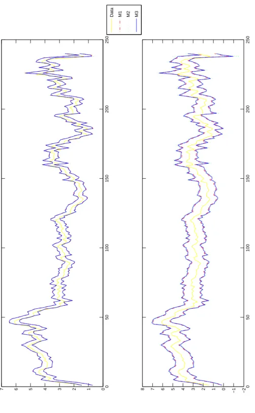
The time plots of recursively estimated parameters ν ˆ

2

and ν ˆ

3

are contained in Fig- ure 1 which reveals that the estimates of ν

2

and ν

3

decrease over time, suggesting that inflation has fatter tails towards the end of the sample.

In line with Clements and Smith (2000) and Diebold et al. (1998) we do not per- form diagnostic tests on the estimated models, and we ignore parameter estimation uncertainty. This approach is not uncommon in the forecast evaluation literature, where the forecasts are considered to be the primitives. In essence, we are sequen- tially conditioning on the information generating the forecasts.

To evaluate the sample of density forecasts, we utilize the method proposed by Diebold et al. (1998), which is based on the idea that a density forecast can be con- sidered optimal if the model for the density is correctly specified. This approach allows one to evaluate forecasts without the need to specify a loss function, and in this sense it represents an improvement over most standard techniques for evalu- ating point forecasts, which typically assume quadratic loss.

The method considers the sequence of probability integral transforms of infla- tion with respect to the density forecasts, that is

z

_t

=

Z yt

−∞

p

_t

(u)du, t = 1, ..., T (15) where y

_t

is the realization of inflation at time t and p

_t

(y

_t

) the estimated density fore- cast. Diebold et al. (1998) show that, if the sequence of density forecasts is correctly specified, the corresponding sequence of probability integral transforms z

_t

’s is i.i.d.

U(0, 1). This result suggests evaluating the density forecasts { p

t

(y

t

) }

^Tt=1

by testing the hypothesis of i.i.d. U(0,1) for the sequence { z

_t

}

^Tt=1

.

As Diebold et al. (1998) point out, the fact that the i.i.d. U (0, 1) hypothesis on the z

t

’s is a joint hypothesis makes it difficult to sort out the causes of a possible rejection. We therefore consider a number of tests of the i.i.d. U (0,1) hypothe- sis, ranging from formal tests to more informal, graphical tests. To test the joint hypothesis of U(0,1) and identical distribution, we implement the Kolmogorov- Smirnov (KS) test; to test the i.i.d. hypothesis alone, we consider the BDS test (Brock, Dechert, Scheinkman and LeBaron, 1996), the CK test of time reversibility (Chen and Kuan, 2002) and the Breusch-Godfrey LM (LM) test for serial correla- tion up to 10 lags in the series

⁴

(z

t

− z)

ⁱ

, i = 1, ..., 4.

4The LM test of serial correlation in the series(zt−z)ⁱ,i=1, ...,4is designed to detect misspecifica-

To assess uniformity, we consider the histogram plot of the z’s, and evaluate its distance from the theoretical p.d.f. of a U(0,1) . We accompany the estimates of the p.d.f. by 95% confidence intervals. The derivation of confidence intervals is made possible by the fact that under the hypothesis of i.i.d. U(0,1) the number of obser- vations that fall into a given bin (against all other bins combined) is distributed as a Binomial(T,

_N¹

), where T is the sample size and N the number of bins.

To further evaluate and compare the forecast performance of the three distribu- tions we consider the sequence of time-varying 75% and 99% forecast confidence intervals implied by the three density forecasts of inflation, along with the real- izations of inflation over the out-of-sample period. We also formally evaluate the performance of the three interval forecast series by conducting a test of correct cov- erage (Kupiec, 1995), which establishes whether the realizations of inflation fall within the confidence interval a proportion of times that equals the interval’s nom- inal coverage (i.e., 75% and 99%).

⁵

4.3 Results

For each model of inflation, we test the null hypothesis of i.i.d. U (0,1) for the se- quence of probability integral transforms { z

t

}

t²⁴⁰=1

of the realizations of inflation with respect to the density forecasts generated by each of the three models described in section 4.1.The results for the KS test are reported in Table 1; results for the BDS test, the CK test, and the LM test are reported in Table 2. Finally, Table 3 reports the results of the test for correct coverage of the 75% and 99% interval forecasts of in- flation. The empirical p.d.f. and c.d.f. are shown in Figure 2. The interval forecasts are shown in Figure 3.

4.3.1 Model 1: Normal disturbances

Table 1 reveals that the KS test leads to rejection of the hypothesis of i.i.d. U(0,1) for the series of z’s, at the 5% confidence level. Rejection of uniform distribution is also confirmed by the histogram of the z ’s (Figure 2), which is characterized by some bins that fall outside the 95% confidence interval.

Regarding the hypothesis of independence, Table 2 reveals that both the BDS test and the CK test fail to reject the hypothesis of independence. However, the LM

tions in the conditional mean, variance, skewness and kurtosis.

5 Leta= (1/T)∑^Tt=11(Y_t+1∈CI) denote the empirical coverage and let αbe the nominal cov- erage. Then the relevant null hypothesis is H0 : a=α and the likelihood ratio test statistic is LR=2[log(a^Ta(1−a)^T−Ta)−log(α^Ta(1−α)^T−Ta)],which has an asymptoticχ²1distribution.

10

Table 1: Kolmogorov-Smirnov test of H

₀

: { z

_t

} ∼ i.i.d.U(0,1).

Model Test Statistic p-value

M1:ARMA(1,1)-ARCH(1)-nor 0.0896

^∗

0.0398 M2:ARMA(1,1)-ARCH(1)-t

ν2

0.0923

^∗

0.0313 M3:ARMA(1,1)-ARCH(1)-t

_ν3

(µ,σ) 0.0796 0.0906

Values of the test statistic and p-values for the Kolmogorov-Smirnov test of the hypothe- sis of i.i.d.U(0,1)of the probability integral transforms from each model. A ‘^∗’ indicates rejection of the null hypothesis at the 5% confidence level.

Table 2: p-values of BDS test, CK test and LM test.

BDS test of H

0

: { z

t

} ∼ i.i.d.

Model p-value

M1:ARMA(1,1)-ARCH(1)-nor 0.167 M2:ARMA(1,1)-ARCH(1)-t

ν2

0.233 M3:ARMA(1,1)-ARCH(1)- t

_ν3

(µ, σ) 0.233 CK test of time reversibility

Model p-value

M1:ARMA(1,1)-ARCH(1)-nor 0.3575 M2:ARMA(1,1)-ARCH(1)-t

_ν2

0.3948 M3:ARMA(1,1)-ARCH(1)- t

_ν3

(µ, σ) 0.3252 LM test of no serial correlation in (z

_t

− ¯z)

^k

, k = 1, ..., 4

Series

Model (z

t

− ¯z) (z

t

− ¯z)

²

(z

t

− ¯z)

³

(z

t

− ¯z)

⁴

M1:ARMA(1,1)-ARCH(1)-nor 0.0003

^∗

0.0027

^∗

0.0017

^∗

0.0002

^∗

M2:ARMA(1,1)-ARCH(1)- t

_ν2

0.0004

^∗

0.0038

^∗

0.0025

^∗

0.0003

^∗

M3:ARMA(1,1)-ARCH(1)-t

ν3

(µ, σ) 0.0004

^∗

0.0058

^∗

0.0011

^∗

0.0003

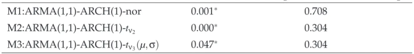
^∗ p-values for: BDS test of independence implemented using the Matlab routine bds.m of Ludwig Kanzler (1998); CK test of time reversibility up to 10 lags (setting the user-defined constant beta equal to 0.5); Breusch-Godfrey LM test of serial correlation up to 10 lags in the series(zt−z)^k,k=1, ...,4, with test statistic computed as the number of observations times the (uncentered)R²from a regression of the series on 10 of its lags. A ‘^∗’ indicates rejection of the null hypothesis at the 5% confidence level.

Table 3: Test of correct coverage of interval forecasts.

p-value

Model 75% nominal coverage 99% nominal coverage

M1:ARMA(1,1)-ARCH(1)-nor 0.001

^∗

0.708

M2:ARMA(1,1)-ARCH(1)-t

_ν2

0.000

^∗

0.304

M3:ARMA(1,1)-ARCH(1)- t

_ν3

(µ,σ) 0.047

^∗

0.304

p-values for test of correct coverage (Kupiec,1995) of 75% and 99% interval forecasts de- rived from the three models. A ‘^∗’ indicates rejection of the null hypothesis of correct cov- erage at the 5% confidence level. See footnote5for details.

test detects serial correlation in all powers of (z

_t

− z), overturning the conclusion of the BDS and the CK test (possibly due to low power of the BDS and the CK tests).

From Table 3, we see that Model 1 fails the test of correct coverage for the 75%

interval forecast, while it does not fail the test for the 99% interval forecast, at 5%

confidence level.

Overall, Model 1 fails on all counts, poorly capturing the dynamics of inflation and assuming a functional form which appears to be misspecified.

4.3.2 Model 2: Student’s t disturbances

As in the case of Model 1, Table 1 shows that the KS test rejects the null of i.d.

U(0, 1) of the z’s derived from the model, at the 5% confidence level. The analysis of the histogram also suggests that the assumption of standard t disturbances does not achieve significant improvements relative to the assumption of normality. The appearance of the p.d.f. plot for Model 2 is very similar to that for Model 1, with some of the bins in the histogram falling outside the 95% confidence interval.

The results of the test for independence also mirror those for Model 1: the BDS and the CK test fail to reject the hypothesis of independence, while the LM test finds serial correlation in the first four powers of (z

_t

− z).

From the perspective of interval forecast performance, the 75% interval fore- casts from Model 2 fail the test of correct coverage, whereas the 99% interval fore- cast has correct coverage, as can be seen in Table 3.

Overall, Model 2 seems not to improve on the performance of Model 1, leading to the conclusion that the standard t -distributional assumption appears overall to be inadequate.

12

4.3.3 Model 3: Scaled and shifted t disturbances

Unlike the case of the previous two models, the KS test fails to reject the null hy- pothesis of i.d. U(0,1) for the sequence of probability integral transforms derived from Model 3, at the 5% confidence level. The apparent superiority of Model 3 over the normal and the standard t is further confirmed by an analysis of the histogram plot in Figure 2, which displays all but one bin falling within the 95% confidence bounds. Thus the probability integral transforms of the density forecasts generated by Model 3 pass most tests of the U(0,1) hypothesis.

Further, the results in Table 3 suggest that the 99% interval forecasts from Model 3 display correct coverage, and for the 75% interval the hypothesis of correct cover- age is rejected only marginally, with p-value equal to 0.047 (in contrast to p-values equal to 0.001 and 0.000 for Models 1 and 2).

However, the results for the tests of independence are analogous to those for the previous two models: although the BDS and CK tests fail to reject the hypothesis of independence, the LM test lead to rejection of the null hypothesis.

In conclusion, density forecasts obtained under the assumption of scaled and shifted t disturbances appear to provide the best approximation for the true density of inflation over the sample considered in the paper. This suggests that the scaled and shifted t-distribution constitutes an improvement over the more common as- sumptions of normality or standard t -distribution, which generate forecasts that fail all evaluation tests. Nevertheless, all three models apparently fail to adequately capture the dynamics of inflation, as suggested by the rejection of the hypothesis of independence for the probability integral transforms implied by the model. A possible explanation for this failure could be the fact that we kept the specification of the conditional mean and variance fixed throughout the out-of-sample period, while in practice the dynamics of inflation may have changed substantially over time, making the ARMA(1,1)-ARCH(1) model a poor approximation for the data- generating process.

⁶

5 An Application to Option Pricing

In this section we illustrate the flexibility of mixtures of scaled and shifted densi- ties and the usefulness of having closed form expressions for the cdf and higher antiderivatives of these densities.

6Given the extent of our specification search, it would not be feasible to conduct a new search for each of the 240 out-of-sample forecast periods.

Under standard assumptions the price of a European call option at time t is given by

C

_t

_{(K) = e}

^−r(T−t)

Z _∞

0

max (0,S

T

− K) f (S

T

) dS

T

(16) where K denotes the strike price, t denotes current date, T the expiration date, r a risk free discount rate, S

_T

the price of the underlying asset at expiration, and f ( · ) the unique risk neutral density of the underlying asset price at expiration. The first term can be interpreted as a discount factor and the integral is just the expected pay- off under the risk neutral probability. For background see e.g. Lamberton and Lapeyre (1996). It is well known in the literature that this risk neutral density can be esti- mated by estimating the option price function C

_t

and then differentiating twice (Breeden and Litzenberger, 1978):

f (S

_T

) = d

²

d K

²

e

^r(T−t)

C

_t

_(K)

K=ST

(17) Specifications for f ( · ) in the literature range from parametric (Melick and Thomas, 1997) and density functionals (Abadir and Rockinger, 2003) to fully nonparametric estimators (Aït-Sahalia and Lo, 1998).

The goal in this section is to derive a closed form expression for the call option price in equation (16) where we assume the risk neutral density to be one of our proposed mixture densities. Once we have a closed form expression, we can then readily estimate the free parameters using suitable nonlinear econometric methods.

We follow Abadir and Rockinger (2003) in extracting risk neutral densities for spe- cific day/maturity combinations which yields a model with one endogenous and one exogenous variable.

Integrating (16) by parts we find that the option price is the integral of the sur- vival function from K to ∞. Solving this integral we find that the call option price can be obtained from

C

_t

_{(K) = e}

^−r(T−t)

_D

⁻¹

_{F (x)}

x=K

. (18) Exploiting the linearity of our mixtures we can thus write the call option price as a convex combination of second antiderivatives of the scaled and shifted t-densities:

c (K; ν,µ,σ, β) = ∑

^q

j=1

β

j

D

⁻²

t

_νj,µj,σj

(x)

x=K

, (19)

where an expression for the second antiderivative of the scaled and shifted t, t

_νj,µj,σj

, is given in Theorem 1. This option price can now be approximated using nonlinear least squares estimation by solving

ν,µ,σ,β

min

∑

q j=1

e

^r(T−t)

C

_t

_{(K) − c(K; ν, µ,σ,β)}

2

.

14

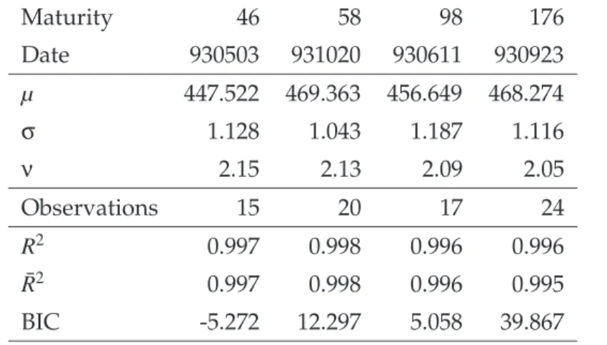
Table 4: Estimation Results for one unrestricted scaled and shifted t kernel.

Maturity 46 58 98 176

Date 930503 931020 930611 930923

µ 447.522 469.363 456.649 468.274

σ 1.128 1.043 1.187 1.116

ν 2.15 2.13 2.09 2.05

Observations 15 20 17 24

R

²

0.997 0.998 0.996 0.996

R ¯

²

0.997 0.998 0.996 0.995

BIC -5.272 12.297 5.058 39.867

Because the approximation is, under regularity conditions, consistent in Sobolev norm (see e.g. Gallant and White (1992)), we can approximate the derivatives of C

_t

_(K) with those of C ˆ

_t

_{(K) = e}

^−r(T−t)

_{c(K; ˆ ν, ˆµ, σ, ˆ β)} ^ˆ _.

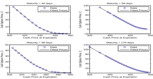
To illustrate the usefulness of our method, we use the data described in Aït-Sahalia and Lo (1998) on European options for 1993. The density functionals of Abadir and Rockinger

(2003) are based on confluent hypergeometric functions and constitute a natural and ambitious benchmark to which to compare our densities. For this reason we pick exactly the same dates and maturities as they do.

Estimation results are reported in Tables 4– 6. Our mixtures of two scaled and shifted t ’s obtain a fit comparable to the density functionals of Abadir and Rockinger (2003) while estimating the same number of parameters (seven) as do their density functionals. Our results are strongly superior to those based on a lognormal den- sity.

Aït-Sahalia and Lo (1998) have argued that estimated risk neutral densities ex- hibit strong kurtosis. Based on our results of Sections 2 and 3, we therefore expect the mixture approach to perform well in this application. When they exist, the mean and the central second to fourth moments of the mixture distribution are given by:

µ

0

≡

Z _∞

−∞

xψ(x)dx =

∑

q j=1

β

j

µ

j

Z _∞

−∞

(x − µ

₀

)

²

ψ(x)dx =

∑

q j=1

β

j

( σ

²_j

ν

j

ν

j

− 2 + (µ

_j

− µ

₀

)

²

)

Z _∞

−∞

(x − µ

0

)

³

ψ(x)dx =

∑

q j=1

β

j

(µ

j

− µ

0

)

( 3σ

²_j

ν

j

ν

j

− 2 + (µ

j

− µ

0

)

²

)

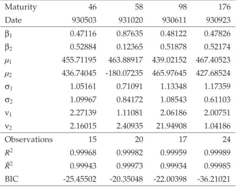
Table 5: Estimation Results for optimal mixture of scaled and shifted t kernels.

Maturity 46 58 98 176

Date 930503 931020 930611 930923

β

1

0.47116 0.87635 0.48122 0.47826

β

2

0.52884 0.12365 0.51878 0.52174

µ

1

455.71195 463.88917 439.02152 467.40523 µ

₂

436.74045 -180.07235 465.97645 427.68524

σ

1

1.05161 0.71091 1.13348 1.17359

σ

2

1.09967 0.84172 1.08543 0.61103

ν

1

2.27139 1.11081 2.06186 2.00751

ν

2

2.16015 2.40935 21.94908 1.04186

Observations 15 20 17 24

R

²

0.99968 0.99982 0.99959 0.99989

R ¯

²

0.99943 0.99973 0.99934 0.99985

BIC -25.45502 -20.35048 -22.00398 -36.21021

Table 6: Estimation Results for Alternative models.

Maturity 46 58 98

Date 930503 931020 930611

Abadir-Rockinger Density Functionals R

²

0.999922 0.999911 0.999661 R ¯

²

0.999864 0.999857 0.999504 Hermite

R

²

0.997214 0.984918 0.993403 R ¯

²

0.996750 0.982764 0.992627 Jumps

R

²

0.997926 0.991013 0.995244 R ¯

²

0.997580 0.989729 0.994685 Mixtures

R

²

0.998267 0.990682 0.996039 R ¯

²

0.997573 0.987577 0.994983 Lognormal Density

R

²

= R ¯

²

0.951508 0.928570 0.980671

These statistics are taken fromAbadir and Rockinger(2003).

16

Z _∞

−∞

(x − µ

0

)

⁴

ψ(x)dx =

∑

q j=1

β

j

( 3σ

⁴_j

ν

²_j

8 − 6ν

j

+ ν

²_j

+ 6σ

²_j

ν

j

(µ

j

− µ

0

)

ν

j

− 2 + (µ

j

− µ

0

)

⁴

)

Our estimation results indicate that not even the second moment exists (cf. Table 5[ν

j

]).

In terms of quality of fit the mixture of scaled and shifted t-distributions is com- parable to the density functionals of Abadir and Rockinger (2003) where the R ¯

²

is higher in the fourth decimal. Our mixture of scaled and shifted t densities clearly outperforms all other methods reported in Abadir and Rockinger (2003) as can be seen from Table 6.

6 Conclusion

We explore convenient analytic properties of mixtures of scaled and shifted t-distributions

that make these well suited for applications to the analysis of economic and finan-

cial time series. Two particularly appealing features of this family are its flexibility

and the fact that it possesses analytically convenient expressions for its antideriva-

tives. We illustrate the usefulness of such features in applications to inflation den-

sity forecasting and to option pricing. In the first application, we show that density

forecasts of inflation obtained using a scaled and shifted t-distribution are more

accurate than forecasts that use the normal or the standard t-distribution. This ap-

plication makes use of the techniques for density forecast evaluation proposed by

Diebold et. al (1998), which rely on computation of the cdf, thus highlighting the

desirability of having convenient expressions for the cdf in such cases. The sec-

ond application replicates results of Abadir and Rockinger (2003), who proposed

a flexible family of distributions and illustrated its usefulness in an application to

option-pricing. We show that the use of our mixture of distributions allows us to

obtain comparably good results, while affording analytical tractability and ease of

implementation. These results suggest that models based on mixtures of scaled

and shifted t -distributions have a useful role to play in econometrics, given their

convenience, generality, and flexibility.

Appendix A Proofs

P

ROOF

of Proposition 1

To establish our result, we take ν > 0 . Consider the general case f (t) = (1 + λt

²

)

^−b

.

with

λ = 1 σ

²

ν b = ν+ 1

2 .

By symmetry and definition of the normalization factor we have κ

_ν,σ

2 =

Z ₀

−∞

(1 + λt

²

)

^−b

dt , so that for x < 0 we can write

F (x) = κ

_ν,σ

2 −

Z x 0

(1 + λt

²

)

^−b

dt ,

and for x > 0 we can write

F (x) = κ

_ν,σ

2 +

Z x 0

(1 + λt

²

)

^−b

dt .

To evaluate the integral, substitute (1 − u) = (1 + λt

²

)

⁻¹

. Then t = λ

⁻¹²

u

¹²

(1 − u)

⁻¹²

dt = 1

2 λ

⁻¹²

u

⁻¹²

(1 − u)

⁻³²

du.

After this substitution the integral becomes:

Z _x

0

(1 + λt

²

)

^−b

dt = 1 2 √

λ

Z ^λx2

1+λx2

0

(1 − u)

^b−3/2

u

^−1/2

du .

This has the form of an incomplete beta integral which can be expressed as a hyper- geometric function (see Erdelyi, Magnus, Oberhettinger and Tricomi, eds (1953), sec- tion 2.5.3), and we obtain

Z _x

0

(1 + λt

²

)

^−b

dt = 1

√ λ

λx

²

1 + λx

²

1/2 2

F

1

1 2 , 3

2 − b; 3 2 ; λx

²

1 + λx

²

.

We can now write F(x) as F(x) = κ

_ν,σ

2 + sign (x) 1

√ λ

λx

²

1 + λx

²

1/2 2

F

₁

1 2 , 3

2 − b; 3 2 ; λx

²

1 + λx

²

.

18