Dissertation
zur Erlangung des Doktorgrades
der Mathematisch-Naturwissenschaftlichen Fakult¨at der Christian-Albrechts-Universit¨at zu Kiel
vorgelegt von
Franziska Ulrike Schwarzkopf
Kiel, 2016
Referent: Prof. Dr. Claus W. B¨oning
Koreferent: Prof. Dr. Peter Brandt
Tag der m¨undlichen Pr¨ufung: 08.06.2016
Zum Druck genehmigt: 08.06.2016
gez. Prof. Dr. Wolfgang J. Duschl, Dekan
Dieses Modellsystem basiert auf dem Modellcode von NEMO unter Verwendung von AGRIF. In den relevanten Regionen, dem tropischen Atlantik und dem tropischen Pazifik, wurde jeweils ein sogenanntes Nest mit einer horizontalen Aufl¨osung von 0,1◦ entwickelt, das in eine globale Mo- dellkonfiguration mit einer horizontalen Aufl¨osung von 0,5◦ eingebettet ist. Simulationen, in de- nen atmosph¨arische Randbedingungen von 1948 bis 2009 zum Antrieb der verschiedenen Modell- konfigurationen genutzt werden, bilden die Grundlage f¨ur die vorliegende Analyse der physikalischen Ventilation der SMZ. Die in den genesteten Modellkonfigurationen simulierte Zirkulation kommt in vielen Aspekten der beobachteten sehr nahe und stellt eine deutliche Verbesserung im Vergleich zur grobaufgel¨osten Simulation dar.
Das Hauptaugenmerk der Analysen liegt auf den Ursprungsregionen und dem Alter des Wassers in den SMZ sowie auf den Pfaden, die dieses Wasser zur¨ucklegt, bevor es in die SMZ gelangt. Zwei Methoden werden verwendet: eine Lagrangesche R¨uckverfolgung von Partikeln, welche sich zu einer bestimmten Zeit in den SMZ befinden, und eine Verfolgung von Oberfl¨achenwasser mithilfe zweier sogenannter “Tracer”, einem Farbstofftracer, welcher die Konzentration eines an der Oberfl¨ache ges¨attigten Stoffes simuliert, und einem Alterstracer, der die Zeit angibt, die seit dem letzten Kon- takt eines Wasserpaketes mit der Oberfl¨ache vergangen ist. Die beiden Methoden beleuchten einer- seits das Ende und andererseits den Anfang der Ventilationspfade in die SMZ und k¨onnen teilweise zu einem vollst¨andigen Pfad zusammengef¨uhrt werden.
Als Ursprungsregionen des Wassers in den SMZ im Atlantik und Pazifik stellen sich die subtropi- schen Becken der jeweiligen Ozeane heraus, mit einem gr¨oßeren Beitrag aus dem S¨uden als aus dem Norden. Konvektionsgebiete in der Weddellsee und f¨ur die SMZ im Atlantik zus¨atzlich im Nord- atlantik tragen ebenso zur Ventilation bei. Die Hauptpfade des Wassers, das in die SMZ gelangt, f¨uhren aus den Subtropen ¨uber die Westr¨ander der Becken in die ¨aquatorialen Stromsysteme und in diesen s¨udlich beziehungsweise n¨ordlich des ¨Aquators nach Osten. F¨ur die s¨udliche der SMZ im Pazifik stellt sich zus¨atzlich ein flacher Pfad dar, der direkt aus dem tropischen Ostpazifik kommt.
tal resolution of the tropical Atlantic (TRATL01) and the tropical Pacific Ocean (TROPAC01) are developed, that are embedded in global 0.5◦ configurations (ORCA05) via two-way nesting provided by Adaptive Grid Refinement in Fortran. The nesting approach allows to simulate relevant small scale processes in the regions of main interest while maintaining the global context. The analysis of the ventilation processes affecting the OMZs is based on hindcast experiments for the period from 1948 to 2009, forced with prescribed atmospheric conditions as given by the Coordinated Ocean Ref- erence Experiment II forcing set. TRATL01 and TROPAC01 show a high fidelity in representing the circulation in the respective tropical ocean basins and better compare to observations than ORCA05.
The main goal of this study is to identify the pathways, source regions and age of the waters in the OMZs. To decipher these aspects, Lagrangian trajectory analyses in conjunction with passive tracer simulations reflecting a surface dye and an artificial age tracer are utilized. The tracers and trajectories implemented here give insights on both, the beginning and the end, of the path of a water parcel from the surface into the OMZs, respectively. They can occasionally be connected, providing the full path.
For both OMZs, either in the Atlantic or in the Pacific Ocean, the subtropics of the respective ocean basin are identified as the dominating source regions with a larger contribution from the South than from the North. Additionally, convection sites in the Weddell Sea and in the northern Atlantic are part of the source regions for waters ventilating the OMZs, where the latter region contributes only to the ventilation of the Atlantic OMZs. It is shown, that in both ocean basins the main supply route of well ventilated waters from the subtropics into the OMZs is via the western boundary and the al- ternating zonal current bands spanning the entire tropical region. Generally, the pathways as well as the source regions for the northern and southern OMZs within the respective ocean are very similar, except for the very last part of the paths, when waters cross the basin from the western boundary to the East on different sides of the equator. In the southern tropical Pacific Ocean, an additional shallow path occurs, directly connecting the eastern tropical Pacific with the southern OMZ.
2.1.4. Regional grid refinement by two-way nesting . . . 15
2.1.5. Model configurations and experiments . . . 17
2.1.6. Caveats of the nested configurations . . . 21
2.1.7. Passive tracers . . . 25
2.2. Computational requirements . . . 27
2.3. Analysis of Lagrangian particle spreading . . . 29
2.3.1. Particle release . . . 29
2.3.2. Qualitative and quantitative experiments . . . 29
2.3.3. Forward and backward integrations . . . 30
2.3.4. Particle populations . . . 30
3. Assessment of spatio-temporal variability 31 3.1. Sea surface height variability in the tropical oceans . . . 32
3.1.1. Observational data sets . . . 32
3.1.2. Sea surface height variability: model vs. observations . . . 32
3.2. Sensitivity study in the Indo-Pacific . . . 37
3.2.1. Introduction . . . 37
3.2.2. Model Experiments . . . 38
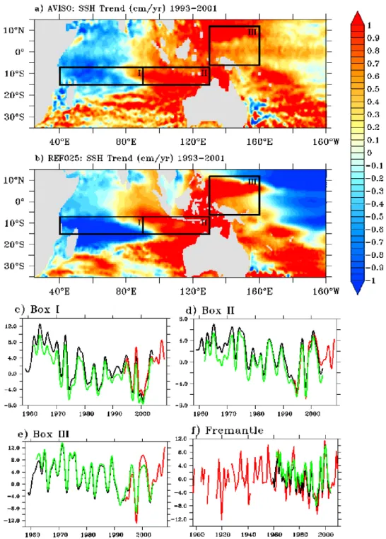
3.2.3. Interannual Variability and Multi-decadal Trend of Sea Level and Heat Content 39 3.2.4. Causes of Sub-surface Cooling in the South Tropical Indian Ocean . . . 40
3.2.5. Concluding Discussion . . . 47
3.3. The 23◦W section . . . 48
3.3.1. Mean spatial structure . . . 48
3.3.2. Temporal variability . . . 54
3.4. Regional tracer spreading . . . 57
3.5. Tropical south east Pacific Ocean . . . 60
3.5.1. Zonal current structure . . . 60
3.5.2. Variability in zonal currents . . . 64
3.5.3. Sea surface height and meridional currents . . . 71
3.6. Benefits from increased horizontal resolution . . . 75
3.6.1. Tropical Atlantic Ocean . . . 75
3.6.2. Tropical south east Pacific Ocean . . . 78
4. Global ventilation processes 83 4.1. Mean circulation in ORCA05 . . . 84
4.2. Passive tracers in ORCA05 . . . 87
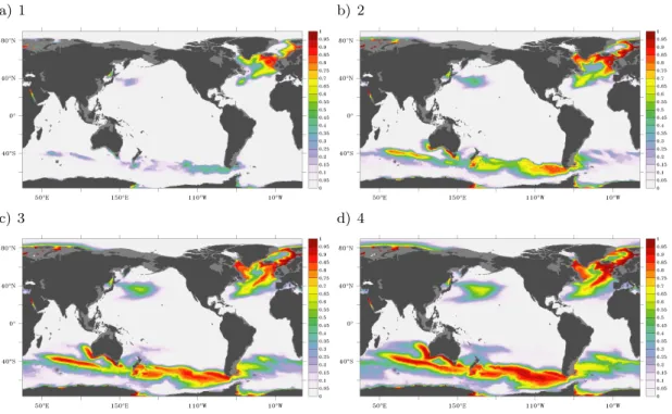
4.2.1. Surface concentration dye (CONC) . . . 87
4.2.2. Time since the last surface contact (AGE) . . . 90
4.2.3. Comparison with the observed oxygen distribution . . . 94
4.3. Tracers in the nested models . . . 96
4.3.1. Comparison of tracers in ORCA05 and the nested models . . . 96
4.3.2. Tracer distribution in and around the OMZs . . . 99
5. Ventilation of the eastern tropical Atlantic 105 5.1. Mean circulation in the eastern tropical Atlantic . . . 106
5.1.1. Vertical velocities in TRATL01 . . . 110
5.2. Ventilation pathways assessed by particle trajectories . . . 113
5.2.1. Pathways into the northern OMZ . . . 123
5.2.2. Pathways into the southern OMZ . . . 130
5.3. Integrated Lagrangian pathways . . . 136
6. Ventilation of the eastern tropical Pacific 143 6.1. Mean circulation in the eastern tropical Pacific . . . 144
6.1.1. Vertical velocities in TROPAC01 . . . 146
6.2. Ventilation pathways assessed by particle trajectories . . . 151
6.2.1. Pathways into the northern OMZ . . . 161
6.2.2. Pathways into the southern OMZ . . . 168
6.3. Integrated Lagrangian pathways . . . 174
7. Summary and conclusions 179 7.1. Methodological aspects . . . 180
7.2. Representation of circulation features in the models . . . 181
7.3. Ventilation of the OMZs . . . 182
7.4. Connection of tracers and trajectories . . . 184
7.5. Comparison between Atlantic and Pacific . . . 185
7.6. Final remarks . . . 186
Bibliography 189
A. Appendix 203
Contents
1.1. Ocean ventilation and Oxygen Minimum Zones . . . . 2 1.2. Need for an efficient model system . . . . 5 1.3. Structure of the study . . . . 7
In the corners at the bottom of the pages, flipbooks show 80 years of the paths of particles from the mixed layer into the northern (red) and southern (black) Oxygen Minimum Zones in the tropical Atlantic (odd pages) and Pacific (even pages) Oceans. The depth of the particles is given by the blue colourscale.
To see the particle move from the mixed layer into the OMZs in the Atlantic Ocean, use your left thumb, starting at the last page. For the pathways into the OMZs in the Pacific Ocean, use your right thumb, starting at the first page.
1.1. OCEAN VENTILATION AND OMZS CHAPTER 1. INTRODUCTION
1.1. Ocean ventilation and Oxygen Minimum Zones
Ocean ventilation is a major process affecting marine life [e.g. Brewer and Peltzer (2009)] as well as the climate system [Bryan et al. (2006)]. Upper Ocean waters with properties determined by the atmospheric conditions above [Liss and Merlivat (1986); Phillips (1994)] are transported down- ward, renewing the interior and deep Ocean waters [Khatiwala et al. (2012)]. Oxygen, carbon dioxide (CO2) and other soluble gases are carried with these waters and the ventilation therefore is of fundamental importance for their uptake and storage within the ocean. Ventilation timescales range from decades to centuries and millennia [England (1995); Haertel and Fedorov (2012); Holzer and Hall (2000)]. Depending on the different time scales the supply with these substances differs regionally, leading to diverse conditions with zones of high and low concentrations of the various substances. The partly long temporal scales make the ventilation a factor in building poorly oxy- genated zones [Luyten et al. (1983)] and that remotely controls the climate.
The ventilation is responsible for the supply of the interior Ocean with nutrients and elements needed for biogeochemical cycles including oxygen and CO2 and also plays a buffering role for the climate in storing green house gases for long times. The oceanic uptake of gases at the surface is mainly determined by the temperature in the surface waters and by partial pressue gradients between the atmosphere and the ocean, the so called solubility pump [Phillips (1994); Takahashi et al. (2002)]. Regions with lower temperatures show higher solubilities and are therefore more effective in drawing down atmospheric CO2. The gas concentrations that are set at the surface are transported with the water parcel into the ocean. During its residence time below the surface, on its way through the interior ocean it is affected by biogeochemical processes, altering the concentrations of these gases and nutrients within the water through biological production and consumption or by other chemical transformations [e.g. Denman et al. (2007)]. In upwelling areas, where nurtrient rich waters reach the surface, CO2 is outgassed to the atmosphere. Under global warming, the Ocean might regionally change its role from a CO2 sink into a CO2 source [Takahashi et al. (2012); Gruber et al. (2009)]. When a water parcel returns to the surface after up to hundreds or thousands of years and again interacts with the atmosphere, the concentrations and solubilities might then have changed. The gradient between the ocean and the future atmosphere could have reversed and a positive feedback might come into play, accelerating global warming [Cox et al. (2000); Sarmiento and Qu´er´e (1996)].
Dissolved oceanic oxygen is determined by the same physical processes as CO2, but in contrast it is not affected by changes in its atmospheric concentrations. Along the way of a water parcel through the ocean, oxygen concentrations are evolving due to physical (mixing) and biological (pro- duction and consumption) processes, even in abyssal layers [Craig (1971)]. Changes in the oxygen supply define and alter habitats of marine organisms that depend on the abundance of oxygen [e.g.
Stramma et al. (2012)]. In poorly ventilated regions, the so called shadow zones [Luyten et al.
(1983)], where ventilation timescales are extraordinarily long for intermediate depth ranges and the supply with oxygen is low, co-occurring with high biological productivity and therefore, high oxygen
through outgassing, be of relevance for the climate [Gleßmer et al. (2011)] and has already been shown to increase [Ar´evalo-Mart´ınez et al. (2015)]. Changes in the strength and extent of the poorly oxygenated waters are therefore affecting CO2 and other green house gas concentrations, not only locally but, via the large scale circulation, also globally.
It is under debate, how ocean ventilation changes under global warming conditions. Keeling and Garcia (2002) expect, that ventilation and oxygen concentrations decrease while model results by Gnanadesikan et al. (2007) show that in poorly ventilated regions, oxygen concentrations might increase under global warming. Yamamoto et al. (2015) differentiate between centennial scale re- duction in oxygen concentrations and a recovery of deep ocean oxygenation on millenial timescales, that later on lead to an increase in oxygen concentrations. In some low oxygen areas, including the southern Atlantic OMZ and at the boundary of the northern Atlantic OMZ as well as the southern Pacific OMZ, Oxygen concentrations have been observed to locally decrease within the period from 1960 to the mid 2000s [Stramma et al. (2008, 2010)]. To investigate the causes of these trends, mechanisms of OMZ ventilation need to be understood first.
The tropical Atlantic and Pacific Oceans are marked by the strong equatorial currents bordered by the poleward limbs of the subtropical gyres [Schott et al. (2004)]. In the eastern parts of these basins, where ventilation happens on long time scales, OMZs are located close to the coast north and south of the equator. The vertical location of these zones is at intermediate depth between
∼300 m and∼700 m. In the Atlantic ocean, minimum oxygen values are higher than in the Pacific Ocean where strongest OMZs are located in the eastern tropics with large spatial extent and even anoxic conditions [e.g. Stramma et al. (2008)].
The oxygen budget within the OMZs is a complex and not yet fully understood interplay between different consumption and supply processes [Karstensen et al. (2008)]. Recently Brandt et al. (2015) gave a broad overview on processes affecting the formation of OMZs as well as mechanisms causing changes within the OMZs, with a focus on the eastern tropical north Atlantic and, to a minor extent, on the eastern tropical south Pacific. Oxygen consumption and supply oppose each other, leading to regionally varying oxygen concentrations, and imbalances between the two cause changes in these concentrations. They summarize, that oxygen consumption is to 80% balanced by the divergence
1.1. OCEAN VENTILATION AND OMZS CHAPTER 1. INTRODUCTION
of meridional eddy and diapycnal fluxes. The remaining 20% can be ascribed to zonal advenction, that cannot be observationally quantified, and to the long-term tendency [Brandt et al. (2015)].
This budget has been observed exemplarily at 23◦W, close to the western boundary of the OMZ in the north eastern tropical Atlantic by Hahn et al. (2014) building on Karstensen et al. (2008) and Fischer et al. (2013). They find that above the deep oxycline advective and zonal eddy processes dominate the supply part of the budget. For the vertical structure of the contributions they find, that in the upper part of the OMZ depth range these factors vanish and below the OMZ core their contribution again grows to values comparable to the meridional eddy and diapycnal supply. Most studies analyzing the advective part of the ventilation process focus on the equatorial currents, that indeed advect oxygen rich waters from the western parts of the basins towards the east [e.g. Brandt et al. (2010)]. However, a connection from the equatorial region into the OMZs, that are located several degrees off the equator, is not shown.
During the revision of the present thesis, a study by Pe˜na-Izquierdo et al. (2015) was published, which examines the pathways of water masses into the north eastern tropical Atlantic OMZ by analyzing a model at an eddy-permitting resolution using a Lagrangian approach. Among their findings, that are in good agreement with what is shown here, they exhibit the importance of north- ern, off-equatorial currents for the ventilation of this OMZ and that the connection between the OMZ and the equatorial region is weak.
The above mentioned studies mainly focus on the OMZ in the north eastern tropical Atlantic and the importance of the zonal equatorial circulation for transporting oxygen-rich waters to the vicinity of the OMZs. They furthermore point to the importance of meridional and diapycnal eddy-driven oxygen supply. The current knowledge about the advective, large scale ventilation processes and their importance for the OMZs, especially for those in the tropical Pacific, is limited. The dif- ferences and similarities in ventilation processes between the Pacific and Atlantic OMZs have not been covered to date. A comprehensive examination of the whole oxygen supply paths from the ventilation at the Ocean surface into the cores of the OMZs is missing. These factors leading to the following questions are subjet to the present study:
• Which currents and circulation features are contributing to the ventilation of the OMZs?
• Where are the source regions of waters entering the OMZs?
• What are the pathways and timescales, waters take to enter the OMZs?
• What are the similarities and where are the differences between the ventilation of the OMZs
way through the world ocean. CFC concentrations can be used as a measure for the age of the water, but only for waters subducted after the CFC introduction [Sonnerup (2001)]. Pathways can additionally be investigated based on drifter and float data [e.g. Carr and Rossby (2001); Grodsky and Carton (2002)], however, these observational attempts are restricted to the instrumental design by e.g. pre-defined drifting depths and limited to short time scales of only up to several years.
On long time scales observational quantities, exhibiting ventilation pathways, especially into poorly ventilated regions like the OMZs are unavailable. Here, Ocean models come into play, providing the framework for analyses beyond observationally available temporal and spatial scales.
To get trustworthy results from analyses based on numerical ocean models, those should be able to realistically simulate the ocean with a variety of processes affecting the ventilation. Convection and subduction play a key role to bring surface waters into the interior ocean [Blanke et al. (2002)], distinct currents transport water masses and mesoscale features contribute to mixing processes [e.g.
Chanut et al. (2008)]. Coarse models with horizontal grid sizes of O(1)◦ are able to simulate major features but do not resolve eddies [Houry et al. (1987)]. Although the effect of mesoscale processes is parameterized [e.g. Gent and McWilliams (1990)], these models miss the high spatial variability of the eddy field and its impact on the circulation. These models are mainly used for long integrations spanning centuries to millenia and for coupled ocean-atmosphere or earth system simulations and have been shown to fail in simulating the OMZs [e.g. Deutsch et al. (2011)]; the mesoscale is an important factor in simulating oxygen supply [Gnanadesikan et al. (2013)]. Models with higher (O(0.1)◦) resolutions are still too expensive to do such long integrations and are therefore mostly used for decadal scale simulations. One way to provide a multi-decadal time frame and still simulate mesoscale features is regional modelling at high resolution. The main disadvantage of regional mod- els however, is the loss of feedbacks into the global context. The compromise between integration lengths, spatial coverage and model resolution used within this study is a nesting approach, where distinct regions are simulated at high resolution, embedded via two-way communication in a global model at intermediate resolution [Blayo and Debreu (2006)].
The nesting approach used here is provided by Adaptive Grid Refinement in Fortran (AGRIF) [Debreu et al. (2008)] and allows for flexible implementation of nested regions in different ways.
One-way nesting only provides boundary conditions from the coarse model to the nested region whereas two-way nesting provides the possibility to feed back dynamical effects from the high reso- lution area to the rest of the global ocean during a side-by-side integration of the two. This approach
1.2. NEED FOR AN EFFICIENT MODEL SYSTEM CHAPTER 1. INTRODUCTION
is well established in the field of high resolution ocean modelling and has been used for the inves- tigation of a variety of subjects [e.g. Biastoch et al. (2008); Djath et al. (2014); Fischer et al. (2015)].
The models used within this study are based on the Nucleus for European Modelling of the Ocean (NEMO) code [Madec (2008)]. The configurations are a global configuration at 0.5◦ horizontal res- olution (ORCA05) and two nested configurations with focus on the tropical Atlantic (TRATL01) and the tropical Pacific (TROPAC01) respectively, both at 0.1◦ horizontal resolution in the nested area, embedded in the global ORCA05 configuration. Hindcast and control experiments in all three configurations are performed, forced by atmospheric conditions for the period from 1948 to 2009 [Griffies et al. (2009)].
To follow waters from the surface into the interior ocean and the OMZs in these models, two different methods are applied. The purely advective ventilation is analyzed based on Lagrangian experiments and two passive tracers exhibit a combination of the advective and diffusive parts of the ventilation.
Both of these methods are lacking any biochemical influence and hence provide a purely physical view on the ventilation. In the Lagrangian experiments particles that end up in the northern and southern OMZs in the tropical Atlantic and Pacific Ocean are traced backwards in time towards their source regions over a period of 80 years. The two passive tracers are an ideal age tracer, set to zero at the surface, growing with time elsewhere and a dye, saturated at the surface, spreading into the interior ocean [England (1995)] for a period of 140 years. All these experiments are performed in the global configuration ORCA05 and the nested configurations TRATL01 and TROPAC01 for the respective oceans.
From a process-oriented and methodological point of view, hereafter the following questions arise:
• What is the influence of mesoscale features on the ventilation paths?
• Which methods are suitable to analyze ventilation pathways?
• What can the applied tracers tell about the ventilation and oxygen concentrations?
• What can be gained by the combination of tracers and trajectories?
The models are validated against observations with focus on sea level and the mean circulation and variability in the tropical Atlantic and Pacific Ocean. In the nested model of the tropical Atlantic Ocean a tracer release experiment, that has been done in the real ocean, is reproduced.
Furthermore, a comparison between the nested, high resolution models and the global model at intermediate resolution is given to exhibit the gain from the newly developed configurations when simulating the tropical circulation. A digression to the influence of wind stress over the Pacific Ocean on Indian Ocean heat content and sea level variability on multi-decadal time scales is made to elucidate the ability of the models to reveal distinct mechanisms.
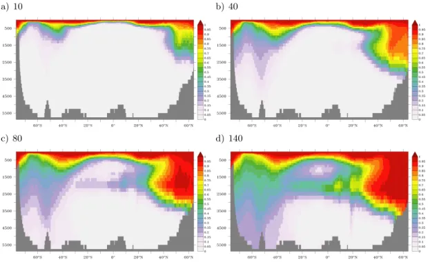
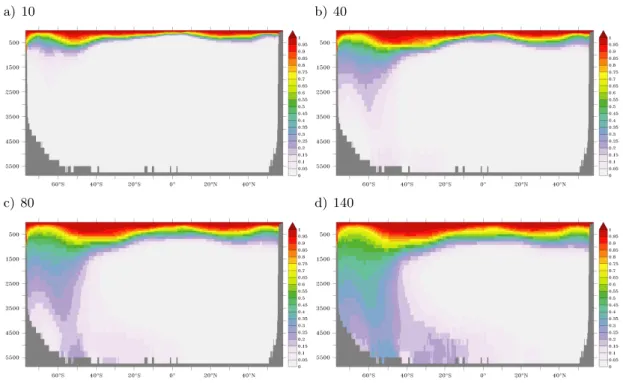
Chapter 4 provides insights on the global ventilation with focus on the OMZs in a 140 years time frame based on passive tracer integrations. The mean circulation in ORCA05 spreading these trac- ers is shown. The evolution of the two passive tracers and their distribution at the end of the integrations is analyzed and compared to those in the nested models. A comparison of the passive tracers to the observed spatial distribution of oxygen that additionally is subject to transformation by biogeochemical processes is made.
In chapters 5 and 6 the advective ventilation of the Atlantic and Pacific OMZs, respectively, is analyzed based on 80 years long Lagrangian backward integrations of particles released in the cor- responding northern and southern OMZs. The mean circulation in the nested models is shown.
Subduction areas, pathways and timescales on which water enters the OMZs are analyzed. Cir- culation features affecting the ventilation are identified and the influence of mesoscale features is assessed.
Chapter 7 summarizes the findings of this study and gives conclusions for the ventilation of the OMZs and suggestions for methodological aspects that arose during this study. A synthetic view on the tracer integrations and the Lagrangian experiments is given, identifying definite and po- tential pathways into the OMZs and source regions of waters entering these zones. A comparison between the ventilation of the Atlantic and Pacific OMZs is given. A brief outlook on methods that ideally would be used to examine the ventilation pathways in future experiments is closing this study.
The appendix A provides enlarged and additional figures, supporting the main part of this study.
2.1. Model architecture . . . . 10
2.1.1. Model framework . . . . 10
2.1.2. Global ocean model configuration . . . . 11
2.1.3. Atmospheric forcing . . . . 13
2.1.4. Regional grid refinement by two-way nesting . . . . 15
2.1.5. Model configurations and experiments . . . . 17
2.1.6. Caveats of the nested configurations . . . . 21
2.1.7. Passive tracers . . . . 25
2.2. Computational requirements . . . . 27
2.3. Analysis of Lagrangian particle spreading . . . . 29
2.3.1. Particle release . . . . 29
2.3.2. Qualitative and quantitative experiments . . . . 29
2.3.3. Forward and backward integrations . . . . 30
2.3.4. Particle populations . . . . 30
2.1. MODEL ARCHITECTURE CHAPTER 2. MODELS AND METHODS
2.1. Model architecture
The model hierarchy developed and used in this study is based on the Nucleus for European Mod- elling of the Ocean (NEMO, section 2.1.1) version 3.1 code [Madec (2008)] in the Drakkar [Barnier et al. (2007)] configuration using an ORCA grid (section 2.1.2). All models are ocean-only models forced by prescribed atmospheric conditions given by the Co-ordinated Ocean Reference Experi- ments (CORE) version 2 (section 2.1.3) [Griffies et al. (2009)] and they are coupled to the Louvain- la-Neuve ice model (LIM2) [Fichefet and Maqueda (1997)]. The models mainly differ in horizontal resolutions from 0.5◦ to 0.1◦, where the highest resolution is achieved regionally, using the two-way nesting approach realized by the Adaptive Grid Refinement In Fortran (AGRIF) [Debreu et al.
(2008)] (section 2.1.4).
2.1.1. Model framework
The NEMO ocean engine provides a framework for diverse applications in oceanic sciences varying in temporal and spatial scales as well as specializations. The ocean circulation model can be used in global or regional configurations with or without coupling to other components like atmospheric or biogeochemical models. NEMO is a primitive equation ocean model derived from the Navier-Stokes equations, using the following assumptions [Stewart (2008)]:
1. Spherical earth: the planet earth is assumed to be an ideal sphere instead of an ellipsoid, where geopotential surfaces are perpendicular to the earth’s radius; gravity is parallel to the radius.
2. Thin-shell: the depth of the ocean is assumed to be negligible small compared to the earth’s radius.
3. Incompressibility: a water volume is constant and cannot be compressed; the divergence of the three-dimensional velocity field is zero; sound waves are excluded.
4. Boussinesq approximation: temporal density variations are small compared to mean density.
5. Hydrostatic approximation: horizontal flow dominates vertical acceleration; pressure gradient only depends on buoyancy and gravity.
The resulting equations are characterized by the prognostic variables temperature, salinity, the full three-dimensional velocity field and sea surface height [Madec (2008)] and discretized in finite dif- ferences on a staggered Arakawa-C grid (figure 2.1) [Mesinger and Arakawa (1976), Arakawa and Lamb (1977)]. The discretization on a staggered lattice should be preferred to avoid smoothing effects that destroy variability on grid scale. The C-grid seeks to minimize the amount of spatial averaging that is needed to calculate the advection of tracers and the horizontal pressure gradient.
The only quantity that includes averaging is the Coriolis term as zonal and meridional velocities
Figure 2.1.:Position of variables in an Arakawa-C grid: T indicates the position, where temperature and salinity (and their derivatives) as well as sea surface height are defined; u,v and w show the location of the three velocity components and f indicates where vorticity is defined. (Figure taken from Madec (2008), figure 3.1)
2.1.2. Global ocean model configuration
The global ORCA configuration developed within the European DRAKKAR collaboration [Barnier et al. (2007)] is the basis for all models used in this work. Its tri-polar, curvilinear horizontal grid allows to simulate the entire ocean without a singularity at the North Pole. This is achieved by replacing the North Pole by two poles, one located in Canada and the other in Russia (figure 2.2 a) while the South Pole does not differ from its geographical position, as it is on land anyway. In the Indian Ocean at 73◦E, the first and the last grid points in zonal direction are located and connected using cyclic boundary conditions. In the vertical, the grid consists of 46 z-levels with increasing thickness ranging from 6 m at the surface to 250 m in the deepest layer. The uppermost 500 m of the water column are covered by 20 layers (figure 2.2 b). Partial cells [Pacanowski and Gnanadesikan (1998)] allow for a better representation of the topography: where necessary, the last cell above the bottom is only partially filled (figure 2.2 c). At least a portion of 25 meters of any cell within the water column has to be filled with ocean, therefore some cells do not fully represent the depth given by the model’s bathymetry (first and sixth column in figure 2.2 c)
The surface is represented in a free linearized filtered sense following Roullet and Madec (2000).
The free surface allows for external gravity waves, that would need a very short time step; with the
2.1. MODEL ARCHITECTURE CHAPTER 2. MODELS AND METHODS
a) Horizontal grid
b) Vertical levels c) Partial cells
Figure 2.2.:Specifics of the ORCA grid: a) horizontal, tri-polar grid, every fifth grid line of an ORCA05 (0.5◦) grid is plotted; b) vertical resolution, indicating the depth of the model layers (black lines) and their thickness (green curve) in meters, the red lines mark every tenth level; c) partial cells along the bottom: the section shows full cells (dark grey) and the partial cells (light grey) according to the model’s bathymetry (black curve); the red curve depicts the topography as given by ETOPO2 [U.S. Department of Commerce and Atmospheric Administration (2006)].
2.1.3. Atmospheric forcing
The initial conditions of the ocean models are no motion and climatological temperature and salin- ity distributions as given by the World Ocean Atlas 1998 climatology with improvements for the Arctic Ocean [Steele et al. (2001), based on Levitus et al. (1998)]. Beginning with this initial state, the models are integrated, forced with atmospheric boundary conditions given by the Co-ordinated Ocean Reference Experiments (CORE) [Griffies et al. (2009)] mainly built on NCEP/NCAR reanal- ysis products merged with satellite products. Bulk formulae, also provided by CORE, connect the atmospheric conditions with the ocean [Large and Yeager (2009)].
Due to varying coverage by observations, the periods of full interannual variability differ among the variables. Full, 62 year coverage is given for wind, air temperature and humidity, whereas the availability for precipitation and radiation is restricted to the last 31 years and 26 years at the end of the forcing period, respectively (see table 2.1). A mean annual cycle of monthly and daily data, respectively, is prescribed for the variables before the period in which interannual variation starts.
The forcing fields are available on a 2◦×2◦ horizontal Mercator grid. Climatological river runoff is applied, representing the most important rivers, whereas coastal runoff is equally distributed around the continents. The forcing fields are provided at different frequencies, ranging from 6-hourly to monthly. Details on the prescribed fields are given in table 2.1.
Two different forcing strategies are applied, “interannual forcing” (IAF) and “normal year forcing”
(NYF). A 62 year long interannually varying data set provides the basis for hindcast experiments, where the ocean’s state during the forcing period is computed. Additionally, a climatological ver- sion, where a “normal year” is repeatedly applied is used to identify the model intrinsic variability and drift. The CORE normal year is an averaged year from almost the full forcing period (from 1948 to 2007) providing a smooth transition between December and January and keeping synoptic variability of a “moderate” year (1995) [Large and Yeager (2004)].
A conjunction of IA and NY forcing is used in a sensitivity study in the Indo-Pacific region where the impact of local versus remote winds on upper ocean heat content in the tropical Indian Ocean is investigated [Schwarzkopf and B¨oning (2011)] (see section 3.2).
2.1. MODEL ARCHITECTURE CHAPTER 2. MODELS AND METHODS
value resolution IA availability interpolation
Zonal wind 10 m above the sea surface 6 hourly 1948 - 2009 bicubic Meridional wind 10 m above the sea surface 6 hourly 1948 - 2009 bicubic Air temperature 10 m above the sea surface 6 hourly 1948 - 2009 bicubic Air specific humidity 10 m above the sea surface 6 hourly 1948 - 2009 bicubic Downwelling short-wave radiation daily 1984 - 2009 bilinear Downwelling long-wave radiation daily 1984 - 2009 bicubic
Rain monthly 1979 - 2009 bilinear
Snow monthly 1979 - 2009 bilinear
Table 2.1.:Forcing fields: the variables and their temporal resolution are given as well as the availability period of interannually varying fields and the applied interpolation method (see section 2.1.3, IOF).
Sea surface salinity restoring is used to partly balance drifts in the oceanic hydrography: the upper- most level (with a thickness of 6.4 m) of the ocean is (very weakly) relaxed towards the sea surface salinity given by the World Ocean Atlas 1998 [Levitus et al. (1998)] on a time scale of 1 year by changing fresh water fluxes accordingly. Details on the effect of different restoring strategies can be found in Behrens et al. (2013).
Interpolation on the fly
The 2◦×2◦forcing fields have to be applied to the underlying model grid. This could be done in two ways: interpolating the data “online” while the model is running (“on the fly”) or “offline” before the model starts. Doing the interpolation offline produces an enormous amount of data because every variable has to be interpolated onto every model grid used. More flexible concerning different model grids (see following sections) and with less memory requirements is the interpolation on the fly where only weights are needed to interpolate data from the original grid of the forcing onto the model grid. These weights are computed using the Spherical Coordinate Remapping and Interpo- lation Package (SCRIP, Jones (1998)): For every single grid cell of the model the weights contain information about the contribution of the adjacent points in the original data. Two methods, bilin- ear and bicubic interpolation, are implemented and two sets of weights are provided to the model and applied to the original forcing fields while the model is running. Whether bilinear or bicubic interpolation is used for the different forcing fields depends on their sign: bicubic interpolation can produce spurious negative values for quantities which are positive definite as, e.g., precipitation and shortwave radiation (compare to table 2.1).
the global base model not only provides boundary conditions for the nest but also receives feedback from it.
Figure 2.3 shows a schematic of the nesting process as described by Debreu et al. (2008): First, the base model (B) is integrated one time step with the length rdt (Bn → Bn+1) forward. Based on the two solutionsBn and Bn+1 the lateral boundary conditions (BC) for the nest (N) are spatially and temporally interpolated (BCintn ). Using these BCs, the nest is integrated forwardρt time steps (length: rdt/ρt). The new conditions along the nest boundary (BCupn+1) is then used to update the base model that is then advanced by the next time step, repeating the described procedure.
A frequency (bcl) is defined, at which the nest not only updates the base model along the nest boundary but also at every base model grid point within the nested domain (BCupn+bcl). (A note on the sensitivity of the choice of bcl is given in 2.1.6.)
Figure 2.3.:Schematic view of the integration procedure with AGRIF. The red grid stands for the base model (B), the blue grid indicates the nest grid (N) and the purple box shows the boundaries of the nested region and its location in the base model. Along these grid lines, the lateral boundary conditions (BC) for the nest are provided from two consecutive time steps (n and n+1) in the base model by interpolation (tilted arrows; indicated asBCint). The base model time step (rdt) is divided by the temporal refinement factor (ρt) to get the nest time step. At Every ρt nest time step, the base model is updated with the new boundary conditions from the nest (BCupρt(n+1)) and at every bcl (so called baroclinic update frequency) time step it receives an update along all grid points within the nested region (BCupn+bcl; purple lines).
The spatial refinement, for stability reasons requires a smaller time step. Although the CFL-criterion suggests a temporal refinement factor of five, here, test integrations show, that stability is still given
2.1. MODEL ARCHITECTURE CHAPTER 2. MODELS AND METHODS
with a factor of four. Additional, horizontal diffusivity (aht0) and viscosity (ahm0) parameters that go into the applied Turbulent Closure Scheme [Madec (2008)] need to be adjusted. The values for the base model are taken from the reference ORCA05 simulations provided by the Drakkar group (aht0 = 600m2/s and ahm0 =−12·1011m4/s) and for the nested regions they are adopted from Biastoch (2008) (aht0 = 200m2/sand ahm0 =−2.125·1010m4/s).
To assure a smooth transition of signals from the nest into the base region, a “sponge layer” is applied along the boundaries of the nest. Small scale features moving undamped into the coarse region would cause instabilities or reflections at the boundaries. Therefore an additional viscosity term is applied on tracers and momentum in the first and last grid boxes within the nested domain.
The coefficient used here is 2160m2/s.
Nest preparation
The “nesting tools” are Fortran95 based programs to interpolate between different grids [Lemari´e (2006)]. Here, they are used to produce input data defining grids and bathymetry as well as inter- polated restart and forcing fields for the nested region of the model.
The input data given to the nesting tools are the coordinates field from the base model including all horizontal grid information, bathymetry files from the base model and ETOPO2 [U.S. Department of Commerce and Atmospheric Administration (2006)] as well as data that need to be available on the nest’s grid. Those data together with a namelist, describing the position and refinement factors as well as some characteristics of the nest and base model (e.g. partial cells) are used to create nest specific data to run the model.
In a first step a coordinates file for the nest, depending on it’s position within the base model and the refinement factors is built, using fourth order polynomial interpolation. Three grid cells along the boundaries are coarse in the nest and used to connect to the base model. Based on this grid infor- mation and a high-resolution topography (ETOPO2, downloaded from http://www.ngdc.noaa.gov/
mgg/fliers/06mgg01.html) the bathymetry of the nest is interpolated by median averaging all high- resolution grid points within one grid cell of the nest. The bathymetry is then connected to the one of the base model: using partial cells, it is ensured, whether the three coarse boundary grid cells are at the same level as the coarse bathymetry. Finally the bathymetry is smoothed to avoid too sharp gradients using a hanning filter. For the base model, an updated bathymetry is created to allow for two-way exchange between the grids, turning land points on the base model grid to ocean points if they include ocean in the nest bathymetry.
Initial conditions (temperature and salinity) as well as the runoff and sea surface salinity (used for restoring) fields are then interpolated from the coarse grid onto the nest via bicubic interpolation.
All configurations are based on the ORCA grid as described in section 2.1.2. The specifics of the distinct configurations will be introduced in the following.
Configurations
The standard configuration here is an ORCA05 setup with 0.5◦nominal horizontal resolution leading to a grid size of 55 km at the equator gradually decreasing to 20 km near the poles. This interme- diate resolution model does not explicitly resolve eddies [Houry et al. (1987)], but their effective flattening of isopycnal surfaces is accounted for by a lateral eddy induced velocity parameterization (GM) [Gent and McWilliams (1990)].
Nested AGRIF configurations for the Tropical Atlantic (TRATL01) and Pacific (TROPAC01) at 0.1◦ resolution are developed and used in this study to investigate ventilation processes, affecting the oxygen minimum zones in the eastern parts of these ocean basins. In the Atlantic Ocean, the nest extends from 30◦S to 30◦N, spanning the basin from 70◦W to the African continent at 18◦E (figure 2.4 a). The nest in the Pacific Ocean spans the entire basin, between 49◦S and 31◦N in- cluding Australia and New Zealand, and reaches from the coast of South America (60◦W) into the Indian Ocean up to 73◦E (figure 2.4 b), where the cyclic folding line of the ORCA05 grid is located (crossing that line with a nest is technically not possible yet).
Additional configuration:
The Fukushima Daiichi nuclear power plants were destroyed by the magnitude 9.0 T¯ohoku earth- quake and subsequent Tsunami hitting the reactors in March 2011. In consequence, radioactive material was released into the environment. A large amount also entered the Ocean through rain- fall and direct release of contaminated waters from the power plants into the Pacific Ocean off Fukushima. The spread of long living isotopes such as137Cesium over a decade has been addressed by model experiments using different horizontal resolutions, including a dedicated AGRIF configu- ration of the Northern Pacific Ocean, NPAC01. The results have been published in the open access journal “Environmental Research letters”, July 2012: Behrens et al. (2012).
2.1. MODEL ARCHITECTURE CHAPTER 2. MODELS AND METHODS
a) TRATL01
b) TROPAC01
Figure 2.4.:Regional setup of TRATL01 and TROPAC01: Snapshot of speed at 100 m depth in the ORCA05 at 0.5◦horizontal resolution (global fields) with embedded nests at 0.1◦resolution in the tropical Atlantic from 70◦W to 18◦E and 30◦S to 30◦N (TRATL01, a) and in the tropical Pacific from from 73◦E to 63◦W and 49◦S to 31◦N (TROPAC01, b).
Figure 2.5.:Regional setup of NPAC01: Snapshot of speed at 100 m depth in the ORCA05 at 0.5◦ horizontal resolution (global fields) with an embedded nest at 0.1◦resolution in the norther Pacific from 100◦E to 100◦W and from 17◦N to∼60◦N.
Experimental strategy
For each of the three configurations ORCA05, TRATL01 and TROPAC01, two main experiments were performed: an interannually forced hindcast experiment from 1948 to 2009 and a climato- logically forced run, parallel to each of the hindcasts. The latter ones are used to identify model intrinsic variability and trends not caused by the forcing itself. Each of these experiments is pre- ceded by the same 80 years long spin-up experiment in ORCA05 forced with the normal year forcing as provided by CORE-II (see section 2.1.3). The spin-up is used to overcome initial shocks and subsequent adjustment processes due to the initialization with an ocean at rest and climatological hydrography [Kantha and Clayson (2000)]. In the actual analyses of the nested configurations, the first O(10) years are neglected as well, taking into account additional adjustments, when switching to the higher resolution. This time appears to be appropriate in the tropical oceans, based on
2.1. MODEL ARCHITECTURE CHAPTER 2. MODELS AND METHODS
wave dynamics and from time series analyses, not shown here, that exhibit initial trends to vanish after the first ten years. The period of the climatologically forced run in ORCA05 is extended to 200 years. The integration strategy for the experiments used throughout this study is visualized in figure 2.6 and their names are given in table 2.2.
Figure 2.6.:Experimental integration strategy: the ocean state after 80 years of the 200 years long normal-year (NY) forced experiment in ORCA05 (ORCA05-NY) provides the initial conditions for NY experiments in TRATL01 (TRATL01-NY) and TROPAC01 (TROPAC01-NY) as well as interannually (IA) forced hindcast experiments from 1948 to 2009 in ORCA05 (ORCA05-IA), TRATL01 (TRATL01-IA) and TROPAC01 (TROPAC01-IA).
Configuration Internal Name Acronym Initial conditions Forcing
ORCA05 TRC001 ORCA05-NY Levitus NYF 200 yrs
ORCA05 TRC006 ORCA05-IA ORCA05-NY year 80 IAF
TRATL01 TRC001 TRATL01-IA ORCA05-NY year 80 IAF
TRATL01 TRC002 TRATL01-NY ORCA05-NY year 80 NYF 62 yrs
TROPAC01 TRC001 TROPAC01-IA ORCA05-NY year 80 IAF
TROPAC01 TRC002 TROPAC01-NY ORCA05-NY year 80 NYF 62 yrs
Table 2.2.:Model Experiments in ORCA05, TRATL01 and TROPAC01: interannual forcing (IAF) covers the period 1948 to 2009 where the normal year forcing (NYF) can be applied for an arbitrary number of years, indicated in the forcing column.
1. Vertical velocities: to avoid discontinuities in the global model, horizontal velocities are inter- polated from the nest grid onto the base model grid, and only afterwards, vertical velocities are computed, using the continuity equation. Very noisy, unrealistic fields of vertical velocities occur on the base model grid within the nested region (figure 2.7). A series of experiments differing in the frequency (bcl, see section 2.1.4) at which the base model is updated with the information from the nest, shows a reduction of the noise amplitudes when updating the base model more often and an increase when reducing the update frequency. This behaviour, however, only holds for regions with highest variability on grid scale.
a) Base model grid b) Nest grid
Figure 2.7.:Vertical velocity at 100 m depth [10−5m/s] averaged from May to August in an arbitrarily chosen model year, here 2000, from a) the base model and b) the output on the nest grid.
2. Horizontal velocities and MOC: when computing the MOC by integrating meridional veloci- ties, another noisy structure occurs in the base model within the nested region. The meridional velocity itself does not show this noise, but already shows strong alternating structures on grid scale. These are represented by smooth transitions from e.g. positive to negative values in the nest, where in the base model strong negative values are directly neighbouring strong positive values (figure 2.8). Only the integration of these structures leads to unacceptable noise in the MOC on the base model grid.
2.1. MODEL ARCHITECTURE CHAPTER 2. MODELS AND METHODS
a) ORCA05 b) ORCA05
c) Base model grid d) Base model grid
e) Nest grid f) Nest grid
Figure 2.8.:Annual mean (year 2000) meridional velocity [cm/s] at 1000 m depth and MOC [Sv] from an un-nested global ORCA05 simulation a) and b)), the base model of TRATL01 c) and d)) and the nest of that model e) and f)) restricted to the region where the western and eastern boundaries in the nest are on land (between the southern boundary at 30◦S and 10◦N) and therefore allow for MOC computation.
Bold lines in c) to f) mark the limits of the nested region and dashed lines mark the northern limit for MOC calculations in the nest.
To avoid physically unrealistic results due to these inconsistencies in the output fields, the analyses within nested regions will be restricted to the high resolution output of the nests throughout this study. Again, the described behaviour only occurs in the output fields and not during model inte- gration.
in the interannually forced experiment and not in the climatological run. The coarseness of the base model does not allow to represent the coastlines as good as in the nest (figure 2.9 c). Additionally, some narrow bays (e.g. red boxes in figure 2.9 c; locations of overshoots) are represented by only one grid box, leading to problems with the lateral no-slip boundary condition. Whether the imple- mentation of the GM parameterization in the base model that is not necessary in the nest plays a role here, is not further investigated.
The integration time step is chosen relatively long, partly based on considerations concerning the computational costs and might contribute to the issue described here. A reduction of the time step leads to a reduction of the occurrence of the overshoots but does not eliminate them completely. To keep an admittedly dissatisfying balance between the computational costs and the inconsistencies found in TROPAC01-IA the time step for this experiment is divided by a factor of two compared to all the other experiments used throughout this study.
Further investigation after the completion of the experiments in TROPAC01 exhibited a defect in the runoff field used for the nest integration: the applied interpolation method lead to negative val- ues at some narrow bights, that, in later experiments were identified as major contributor causing the overshoots.
As the main focus that TROPAC01 is used for in this study concentrates on the eastern part of the nest and the signal described above does not propagate away from the Philippines, the results are not affected by these inconsistencies but their presence should be kept in mind.
2.1. MODEL ARCHITECTURE CHAPTER 2. MODELS AND METHODS
a)
b) c)
Figure 2.9.:Arbitrarily chosen SST snapshot in TROPAC01: shown in a) is the base model SST with the nest SST overlaid (black box) In the base model the GM parameterization is active to simulate the effect of non-resolved eddies acting to flatten isopycnal surfaces. Due to the higher resolution, this effect is explicitly resolved in the nest, where GM is deactivated. To improve the circulation through the maritime continent, the lateral boundary condition in this area is switched from “free slip”, which is used everywhere else, to “no slip” (blue box). Within this region, in some bays, bathymetric inconsistencies appear, causing unrealistically high/low values of T and S (stars in b)). At these locations (black box in b); area shown in c)) inconsistencies between the nest and the base model bathymetry occur. c) shows the land mask of the base model (grey shading) and the nest (hatched area), indicating problematic bays by the red boxes.
Age tracer
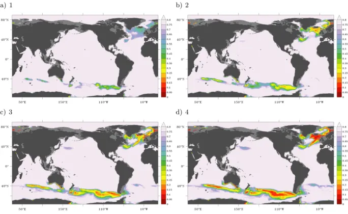
The tracer “AGE” is initialized with 0 everywhere and grows with time except for the surface, where it is held at 0. This formulation defines the time since a water parcel had the last surface contact as its “age”. In general, AGE is only meaningful in equilibrium, when the entire ocean is mixed and AGE does not change anymore. During transition from initialization to equilibrium, AGE changes (even in better ventilated regions) due to mixing processes with other e.g. deeper lying, less ventilated zones [England (1995)]. Although it needs several thousand years to reach such an equilibrium, the tracer AGE is only integrated for 142 years (80 years spin-up plus 62 years hindcast) here, owing to the amount of expensive computing time needed for the integration of such high-resolution models as TRATL01 and TROPAC01 (see section 2.2). The change of AGE over time within the regions of interest for the present study slows down significantly towards the end of these 142 years (figure 2.10 a), however it has to be kept in mind, that the presented AGE values, especially in the poorly ventilated regions, are too low compared to their real age.
a) AGE b) CONC
Figure 2.10.:Schematic evolution of AGE (a)) and CONC (b)) over 140 years of integration from zero-initialization at 100 m (black), 500 m (red) and 2000 m (green) depth. With increasing depth, AGE needs longer to slow down its growth and CONC needs longer to reach a saturated state
2.1. MODEL ARCHITECTURE CHAPTER 2. MODELS AND METHODS
Surface concentration
The tracer “CONC” is initialized with 0 everywhere except for the surface, where it is set to and held at 1. This tracer depicts the concentration of a dye that is saturated at the surface and shows its pathways towards the interior ocean. In well ventilated regions, CONC increases rapidly to sat- uration. In regions where the ventilation is low, CONC increases slowly and only reaches saturation after a few thousand years, when the full ocean is ventilated (figure 2.10 b). CONC is a meaningful quantity already during its evolution and should tend to one in an equilibrated state.
Tracer release experiments
The third sort of tracer used in this study is a dye that can be applied in various ways to track the spreading of a substance injected into the ocean. The tracer is set to one (released) in a certain area for a limited time. Here, this is done to simulate the GUTRE experiment [Banyte et al. (2012)] (section 3.4) and to simulate the possible spread of radioactive contaminated waters released into the Pacific Ocean after the disaster in Fukushima in March 2011 [Behrens et al. (2012)].
The global ORCA05 simulations are partly performed at the computing centre at Kiel University on a NEC-SX8 and SX9 vector machine. Here, 4 CPUs are used to integrate an entire model year within approximately 5.5 hours on the SX8 and 3.5 hours on the SX9 respectively.
The nested experiments and the tracer experiments in ORCA05 are integrated at the North-German Supercomputing Alliance (HLRN) on a SGI Altix ICE with a scalar architecture. The paralleliza- tion in NEMO is done by area decomposition, i.e. the entire model domain is divided into rectangles of several degrees in latitude and longitude where each of them is integrated on one processor com- municating with neighbouring regions via Message Passing Interface (MPI). The MPI processes are the bottle neck in scalability: at some point, the communication between the CPUs takes more time than the integration itself and an increase in the number of CPUs used for the integrations does not lead to a decrease in computing time anymore. This has been tested exemplary with TROPAC01 (figure 2.11). 512 CPUs turned out to provide the best balance between required com- puting resources (given in NPLs (“Norddeutsche Parallelrechner-Leistungseinheit”); proportional to the product of computing time and number of CPUs) and the real time needed to integrate a model year (blue stars).
a) Real time b) Computational time
Figure 2.11.:Scalability of TROPAC01: the real time needed to integrate one model year depending on the number of CPUs is given in a). The red line marks some kind of threshold for the shortest time reachable. b) shows the costs [NPLs/model year], clearly increasing with the number of CPUs. The blue stars mark the chosen 512 CPUs.
2.2. COMPUTATIONAL REQUIREMENTS CHAPTER 2. MODELS AND METHODS
With the infrastructure described above, the time needed to integrate a model year in ORCA05 is about one hour. For the nests the time rapidly increases to about four hours for one model year of TRATL01 and almost twelve hours for a model year in TROPAC01. For the interannually forced TROPAC01-IA experiment, the time step had to be reduced due to instabilities (see section 2.1.6), leading to a doubling of integration time. The models are integrated year-wise, meaning the model needs to be restarted for every year, leading to waiting time between the integrations of two subsequent model years. All in all, a 62 years long hindcast in TRATL01 needs about a month, whereas for TROPAC01 this can take more than three months, depending on the availability of the computers.
2.3.1. Particle release
Particles (or water parcels) can be seeded in basically two different ways:
1. Seeding at exact locations and time: the locations of seeded particles (longitude, latitude, depth) and the point in time, when it is released can be determined directly.
2. Seeding along a section: a closed section (either by land or other sections) is defined along which particles are seeded according to the velocity field into a pre-defined direction. In this way, more particles are going along with stronger currents. Additionally, using this method, hydrographic conditions can be prescribed, that have to be fulfilled for the particle release, e.g. only water within a certain temperature range is tracked.
In this study the first strategy is used to seed particles within a box, independent from the current structure, as the velocity fields in the release areas are rather sluggish and circulation within the release area would not be taken into account by just releasing the particles along the boundaries of a box, as method two would do.
2.3.2. Qualitative and quantitative experiments
Two types of experiments can be performed using ARIANE:
1. Qualitative: a qualitative ARIANE experiment shows the way of particles, seeded at certain locations over the full period of integration. At every time step, the position of each particle is stored. Additionally, hydrographic properties along the particle tracks can be stored.
2. Quantitative: in a quantitative run, particles are seeded along a certain section (see section 2.3.1) and several other sections can be defined along which particles are collected. The way,
2.3. ARIANE CHAPTER 2. MODELS AND METHODS
particles take from one to another section is not stored, but the number of particles, crossing each section as well as the time needed to get from the release position to the end section is stored. Additionally, each particle represents a transport value derived from the velocity field at its release location, so that in the end, transports between two sections can be determined.
Here, only qualitative experiments are used, as most of the measures provided by the quantitative method can be derived within the post-processing, except for the transport that is assigned to each water parcel.
2.3.3. Forward and backward integrations
The motion of the particles is integrated by deriving local streamlines for each time step, provided by the underlying velocity fields, and by moving the particles from their current position along those streamlines to their new location, one time step later. The integration then can be done in two ways:
1. Forward: forward integration shows the fate of particles by integrating them forward in time directly using the velocity output from the models. This is mainly used to examine, where waters (or particles in the water) released at a certain location end up under distinct conditions.
2. Backward: with the backward integration, the origin of particles found at a given location or within certain areas can be found by going backward in time. Technically, this is done by changing the sign of all velocities.
This study mainly uses backward integrations, to find the origin and pathways of water parcels that end up in certain areas.
2.3.4. Particle populations
Following a method developed and published by Gary et al. (2011) to qualitatively analyze the resulting trajectories, particle populations are derived. Therefore, a regular, three dimensional grid is defined and the particle occurrences within the individual boxes during the integration time are counted. The resulting populations provide an integrated measure for pathways and residence times of the traced particles.
Contents
3.1. Sea surface height variability in the tropical oceans . . . . 32 3.1.1. Observational data sets . . . . 32 3.1.2. Sea surface height variability: model vs. observations . . . . 32 3.2. Sensitivity study in the Indo-Pacific . . . . 37 3.2.1. Introduction . . . . 37 3.2.2. Model Experiments . . . . 38 3.2.3. Interannual Variability and Multi-decadal Trend of Sea Level and Heat Content 39 3.2.4. Causes of Sub-surface Cooling in the South Tropical Indian Ocean . . . . 40 3.2.5. Concluding Discussion . . . . 47 3.3. The 23◦W section . . . . 48 3.3.1. Mean spatial structure . . . . 48 3.3.2. Temporal variability . . . . 54 3.4. Regional tracer spreading . . . . 57 3.5. Tropical south east Pacific Ocean . . . . 60 3.5.1. Zonal current structure . . . . 60 3.5.2. Variability in zonal currents . . . . 64 3.5.3. Sea surface height and meridional currents . . . . 71 3.6. Benefits from increased horizontal resolution . . . . 75 3.6.1. Tropical Atlantic Ocean . . . . 75 3.6.2. Tropical south east Pacific Ocean . . . . 78
3.1. SSH VARIABILITY CHAPTER 3. MODEL ASSESSMENT
3.1. Sea surface height variability in the tropical oceans
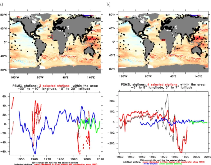
Sea surface height (SSH) in the global ocean is determined by several hydrographic factors like density and heat content as well as the ocean dynamics as consequence of wind induced circulation [Gill and Niiler (1973)]. It therefore offers an integrative measure of the state of the ocean. Glob- ally distributed, partially very long term record, tide gauge stations and satellite altimetry data (AVISO) since the early 1990s provide a large data base for validating the model’s capability of simulating SSH variability and trends. Here, regional SSH anomalies representing the influence of ocean dynamics [Wunsch et al. (2007)] on the sea level are investigated comparing the detrended modelled SSH with both, satellite altimetry and tide gauge data.
3.1.1. Observational data sets Tide gauges
Tide gauges are land based devices, continuously measuring the sea level at a fixed location. The measured sea levels are given relative to a mean state, therefore only sea level anomalies are an- alyzed. Stations around the world (figure 3.1) provide a large database of long term sea level records. The Permanent Service for Mean Sea Level (PSMSL) provides a collection of tide gauge data that are used here to compare modelled and measured sea level variability. This is achieved on a point-wise basis but over a long time, complementing and facilitating the global comparison with short-term satellite measurements (subsection 3.1.1, below). Only quality controlled data are used here [Holgate et al. (2013)].
Satellite altimetry data
Since 1993 several satellite missions measure sea level along their ground tracks using altimetry.
The entire earth (except for the polar regions) is covered by individual tracks roughly every 9 days which are merged to 7-daily fields of sea surface height anomalies. The along track data are mapped onto a grid with 1/3◦ by 1/3◦ resolution. Sea level anomalies are computed using a time averaged reference sea level and are provided by Ssalto/Duacs and distributed by Aviso, with support from Cnes (http://www.aviso.altimetry.fr/ducas).
3.1.2. Sea surface height variability: model vs. observations
A comparison between tide gauge measurements, satellite altimetry and modelled SSH from an ORCA05 experiment is presented here, for the tropical Atlantic Ocean (figure 3.2), the tropical
Figure 3.1.:The locations of the tide gauge stations are given by the black stars. Red circles mark the stations, with records longer than 30 years; blue squares stand for stations with records longer than 60 years.
Areas within the tropical oceans are selected based on the availability of tide gauge measurements, which unfortunately are rare in the regions of interest. Nevertheless, they will be used to investigate the model skill to reproduce local SSH variability. Especially in the tropical Atlantic Ocean (figure 3.2) tide gauge measurements are scarce in space and time. Although the boxes are chosen small (figure 3.2 upper panels), comparing tide gauge and modelled SSH variability within the selected boxes reveals a large discrepancy. The modelled SSH variability (blue curve), except for a minimum in the early 1960s, substantially differs from the SSH variability measured by the tide gauges (red curves). However, comparing the modelled SSH variability within the chosen boxes with AVISO data (green), shows an agreement on interannual time scales. This implies, that the available tide gauge measurements from this region only give insights for the locations of the gauges and are not representative for the surrounding area.
In the tropical Pacific Ocean, the availability of data is much better, mainly due to the presence of several tropical islands, which allow to investigate SSH anomalies not only along the continental coasts but also within the open ocean. Especially in the western part of the tropical Pacific Ocean, within the warm pool region, open ocean tide gauge stations are available. The spread of individual stations is given by the black curves in figure 3.3 a, which show at least one strongly deviating sta- tion. Modelled SSH anomaly within this box goes along very well with the averaged tide gauge time series (red curve) on interannual time scales. A negative linear trend in the modelled SSH causes some tilt of the curves against each other. The agreement between tide gauge (red) and satellite
3.1. SSH VARIABILITY CHAPTER 3. MODEL ASSESSMENT
a) b)
Figure 3.2.:Upper panel: linear trend pattern of SSH over the satellite period from 1993 to 2008 (shading; blueish areas indicate sea level fall, red regions correspond to sea level rise); the locations of all tide gauge sta- tions are indicated by the black stars, the red box indicates the area for which SSH anomaly time series are given below. Lower panel: SSH anomaly time series [mm] from individual tide gauge stations (black curves) and an average of those stations (red thin) as well as a constantly (1.7 mm/yr) detrended time series (red thick) and an acceleratedly (2.6 mm/yr from 1990) detrended time series (red dashed). Mod- elled SSH anomaly within the marked box (blue) and SSH anomaly as measured by satellite altimetry (AVISO, green) are overlaid
altimetry data (green) confirms that the SSH anomaly within the chosen box is represented by the tide gauge measurements, emphasizing the capability of the model to simulate the SSH anoma- lies here. In the eastern tropical Pacific, although the number of tide gauge stations decreases significantly, the available stations are representative for the chosen box there (figure 3.3b). The comparison with AVISO and the model again shows an agreement of the interannual SSH variability.
In the tropical Indian Ocean, the tide gauge data are also quite scarce. Nevertheless, along the
![Figure 3.25.: Zonal velocity [m/s] averaged between 50 m and 100 m (top) depth and 250 m and 300 m (bottom) in February 2002 a) and c) and in February 2009 b) and d) from TROPAC01-IA](https://thumb-eu.123doks.com/thumbv2/1library_info/5482110.1684730/71.892.147.773.310.869/figure-zonal-velocity-averaged-depth-february-february-tropac.webp)
![Figure 3.31.: Meridional velocity [cm/s] from observations (left figures taken from Czeschel et al](https://thumb-eu.123doks.com/thumbv2/1library_info/5482110.1684730/80.892.206.714.172.934/figure-meridional-velocity-observations-left-figures-taken-czeschel.webp)
![Figure 3.32.: Hovmoeller diagram of meridional velocities [cm/s] in 400 m depth at ∼3.6 ◦ S a), 6 ◦ S b) and 14 ◦ S c) in 2009](https://thumb-eu.123doks.com/thumbv2/1library_info/5482110.1684730/82.892.123.804.297.899/figure-hovmoeller-diagram-meridional-velocities-cm-depth-s.webp)