The effect of marine aggregate parameterisations on nutrients and oxygen minimum zones in a global biogeochemical model

(1)

https://doi.org/10.5194/bg-16-3095-2019

The effect of marine aggregate parameterisations on nutrients and oxygen minimum zones in a global biogeochemical model

Daniela Niemeyer, Iris Kriest, and Andreas Oschlies

GEOMAR Helmholtz-Zentrum für Ozeanforschung, Düsternbrooker Weg 20, 24105 Kiel, Germany Correspondence:Daniela Niemeyer (dniemeyer@geomar.de)

Received: 2 April 2019 – Discussion started: 10 April 2019

Revised: 17 July 2019 – Accepted: 25 July 2019 – Published: 15 August 2019

Abstract. Particle aggregation determines the particle flux length scale and affects the marine oxygen concentration and thus the volume of oxygen minimum zones (OMZs) that are of special relevance for ocean nutrient cycles and marine ecosystems and that have been found to expand faster than can be explained by current state-of-the-art models. To investigate the impact of particle aggregation on global model performance, we carried out a sensitivity study with different parameterisations of marine aggregates and two different model resolutions. Model performance was investigated with respect to global nutrient and oxygen concentrations, as well as extent and location of OMZs. Results show that including an aggregation model improves the representation of OMZs.

Moreover, we found that besides a fine spatial resolution of the model grid, the consideration of porous particles, an intermediate-to-high particle sinking speed and a moderate- to-high stickiness improve the model fit to both global distributions of dissolved inorganic tracers and regional patterns of OMZs, compared to a model without aggregation. Our model results therefore suggest that improvements not only in the model physics but also in the description of particle aggregation processes can play a substantial role in improving the representation of dissolved inorganic tracers and OMZs on a global scale. However, dissolved inorganic tracers are ap- parently not sufficient for a global model calibration, which could necessitate global model calibration against a global observational dataset of marine organic particles.

1 Introduction

Oxygen is – beside light and nutrients – fundamental for marine organisms, such as bacteria, zooplankton, and fish. Only few specialised groups can tolerate regions of low oxygen, commonly referred to as oxygen minimum zones (OMZs).

These regions are located in the tropical upwelling regions, where nutrient-rich water enhances primary production and subsequent transport of organic matter to deeper waters, which triggers respiration and consumes oxygen. Together with weak ventilation (which supplies oxygen), this results in oxygen concentrations well below 100 mmol m⁻³. Global models that are used to reproduce OMZ’s volume and location, and their evolution under climate change, differ with respect to the biogeochemical parameterisations as well as with respect to physics (Cabré et al., 2015), resulting in disagree- ments between projected OMZ extent (Cocco et al., 2013).

To date, it is not clear whether these differences can be at- tributed to the differences in the model’s biogeochemistry or the physical models.

One potential parameter affecting distributions of dissolved oxygen and thereby the volume and location of OMZs is the biological carbon pump (Volk and Hoffert, 1985).

Global ocean model studies show that the biological pump is important for the distribution of dissolved inorganic tracers in the ocean (Kwon and Primeau, 2006, 2008) as well as atmosphericpCO₂ (Kwon et al., 2009; Roth et al., 2014).

It further affects the feeding of deep sea organisms (Kiko et al., 2017) as well as the OMZ volume (Kriest and Oschlies, 2015). The biological carbon pump can be subdivided into three components: production of organic matter and biomin- erals in the euphotic surface layer, particle export into the ocean interior, and finally their decomposition in the water column and on the sea floor (Le Moigne et al., 2013). Esti-

(2)

mates of the export of organic carbon out of the surface layer range from 5 to 20 Gt C yr⁻¹, with the large uncertainty illus- trating the gap in our understanding of this process (Henson et al., 2011; Honjo et al., 2008; Keller et al., 2012; Laws et al., 2000; Oschlies, 2001). Further uncertainties are associated with the exact shape of the particle flux profile (e.g.

exponential function vs. power law; Banse, 1990; Berelson, 2002; Boyd and Trull, 2007; Buesseler et al., 2007; Lutz et al., 2002; Martin et al., 1987) and its possible variations in space and time. Recent studies suggest conflicting evidence with regard to the spatial variation of the particle flux length scale (Guidi et al., 2015; Marsay et al., 2015), which may again be influenced by the methodology of estimating the particle flux profile and thus the potential sensitivity to the considered depth (Marsay et al., 2015). Also, the underlying mechanisms for a potential spatio-temporal variation remain unclear: some studies attribute this to variations in temperature and associated temperature-dependent variation in remineralisation (Marsay et al., 2015), while other studies derive this from variations in particle size distributions (Guidi et al., 2015).

One mechanism that leads to a variation in particle size distribution consists in the formation of marine aggregates, which exhibit variable sinking speeds. For example, All- dredge and Gotschalk (1988) and Nowald et al. (2009) found sinking rates for aggregates ranging between 10 and 386 m d⁻¹. Particle sinking speed, and thus the particle flux profile, depends on mineral ballast (Armstrong et al., 2002;

Ploug et al., 2008), porosity and particle size (Alldredge and Gotschalk, 1988; Kriest, 2002; Smayda, 1970). Large particles are associated with high sinking speed and fast passage through the water column, resulting in low remineralisation and thus a small OMZ volume and vice versa. It can therefore be expected that particle aggregation favouring fast sinking speeds can alter the volume of OMZs compared to small particles with low sinking speeds (Kriest and Oschlies, 2015).

However, there are still some gaps in our understanding of the parameters that control the aggregation rate as well as the particle’s sinking behaviour. For example, in situ mea- surements show almost no dependency between diameter and sinking speed (Alldredge and Gotschalk, 1988), whereas aggregates produced on a roller table show a noticeable relationship (Engel and Schartau, 1999). Furthermore, values for stickiness, which defines the probability that after collision two particles stick together, vary over a wide range.

Stickiness depends on the chemistry of the particle’s surface (Metcalfe et al., 2006) and the particle type (e.g. Hansen and Kiørboe, 1997) and ranges between almost 0 and 1 (e.g. All- dredge and McGillivary, 1991; Kiørboe et al., 1990). Thus, aggregation as one process that induces variations in particle size, and thus sinking speed, is only loosely constrained through its parameters.

To explore these relationships further and to examine whether a spatially variable sinking speed improves the fit of a global biogeochemical model to global distributions of dis-

solved inorganic tracers and regional patterns of OMZs, this study uses the three-dimensional Model of Oceanic Pelagic Stoichiometry (Kriest and Oschlies, 2015), coupled with a module for particle aggregation and size-dependent sinking (Kriest, 2002). Given the large uncertainty associated with parameterisations of marine aggregates, we carried out 36 sensitivity experiments in which we varied parameters relevant for particle aggregation and sinking. As in previous studies, the model’s fitness is evaluated by the root mean square error (RMSE) against observational data of dissolved inorganic tracers, namely PO₄, NO₃ and O₂ (Kriest et al., 2017). This study additionally determines the model fitness with respect to extent and location of OMZs, following the approach by Cabré et al. (2015).

To examine the above-mentioned questions, and explore the effects and uncertainties of a model that simulates particle dynamics on a global scale for a seasonally cycling stationary ocean circulation, our main questions are as follows:

1. Does a model that includes explicit particle dynamics improve the representation of observed PO4, NO3 and O2?

2. Does a model that includes explicit particle dynamics improve the representation of observed OMZs, and do the “best” parameters with respect to this metric agree with those constrained by dissolved inorganic tracers?

3. What are the effects of uncertainties in the parameterisation of organic aggregates on model results?

4. Can the assumptions inherent in the model confirm either of the spatial particle flux length scale maps proposed by Marsay et al. (2015) or Henson et al. (2015) and Guidi et al. (2015)?

This paper is organised as follows: we first describe the model and its assessment with regard to dissolved inorganic tracers and OMZs, including the sensitivity experiments carried out with the model. We then present the outcome of the sensitivity experiments, with special focus on the metrics defined above. We finally examine and discuss derived maps of particle flux length scales against the background of maps derived from observed quantities (Henson et al., 2015; Marsay et al., 2015; Guidi et al., 2015).

2 Model description and methods 2.1 Oceanic transport

In this study, we used the “transport matrix method” (TMM) (Khatiwala et al., 2005; Khatiwala, 2007, 2018), as an effi- cient offline method to simulate biogeochemical tracer transport with monthly mean transport matrices (TMs). Addi- tional fields of monthly mean wind, temperature and salinity extracted from the underlying circulation model are used to

(3)

simulate air–sea gas exchange of oxygen and to parameterise temperature-dependent growth of phytoplankton. For our experiments, we used two different types of TMs and forcing fields: one set derived from a coarser-resolution (hereafter called MIT2.8) and one from a finer-resolution version, based on a data-assimilated circulation (ECCO1.0) (Stam- mer et al., 2004). The MIT2.8 forcing and transport represent a resolution of 2.8^◦×2.8^◦and 15 depth layers with a thickness ranging between 50 and 690 m. ECCO1.0 TMs and forcing are based on a resolution of 1^◦×1^◦and 23 depth layers, with a thickness ranging between 10 and 500 m. Further details about the two setups can be found in Kriest and Os- chlies (2013).

In general, we used a time step length of 1/2 d for physical transport and a time step length of 1/16 d for biogeochemical interactions in the coarse resolution, MIT2.8. Because some parameter configurations allow a very large particle sinking speed, which may exceed more than one box per time step, in MIT2.8 we used a biogeochemical time step length of 1/70 d for all simulations withη=1.17 (see Table 1), in the finer resolution, ECCO1.0, we used in all experiments a time step of 1/80 d (see Table 1) but with the exception of three experiments, where we used a length of 1/160 d (these are the experiments for a strong increase of sinking speed with particle size, given by parameterη=1.17; see Table 1). Each model was integrated for 3000 years until tracers approached steady state. The last year is used for analysis as well as misfit calculations.

2.2 The biogeochemical model

2.2.1 Model of Oceanic Pelagic Stoichiometry

The Model of Oceanic Pelagic Stoichiometry, called MOPS (Kriest and Oschlies, 2015), is based on phosphorus and simulates phosphate, phytoplankton, zooplankton, dissolved organic phosphorus (DOP) and detritus. The unit of each tracer is given in millimoles of phosphate per cubic metre (mmol P m⁻³). In addition, MOPS simulates oxygen and nitrate. The P cycle is coupled to oxygen by using a fixed stoichiometry ofR−O₂:P=171.739 and to nitrogen byRP:N= 16.

The stoichiometry of anaerobic and aerobic remineralisation is parameterised following Paulmier et al. (2009). Rem- ineralisation of detritus and dissolved organic matter is fixed to a constant nominal remineralisation rater and is dependent on oxygen but independent of temperature. If oxygen concentrations decrease, denitrification replaces aerobic respiration, consuming nitrate. If neither oxygen nor nitrate is sufficiently available, remineralisation stops as the model does not account for other electron acceptors such as sulfate.

As both forms of remineralisation follow a saturation curve (Monod type), the realised remineralisation rate may diverge from the constant nominal remineralisation rate.

On long timescales, the loss of fixed nitrogen through denitrification is balanced by temperature-dependent nitrogen fixation. Therefore, it should be noted that while phosphorus is conserved, the inventory of fixed nitrogen as well as oxygen is variable and dependent on ocean circulation and biogeochemistry (Kriest and Oschlies, 2015).

In the basic model without aggregation the sinking speed of detritus increases linearly with depth. With constant remineralisation rater, the particle flux can thus be described byF (z)∝z^−b withb=^r

a (Kriest and Oschlies, 2008) and is therefore (for constantr, e.g. in a fully oxic water column) comparable to the common power-law description of observed particle fluxes (Martin et al., 1987). The fraction of detritus reaching the seafloor follows two pathways: one fraction is re-suspended back into the deepest box of the water column, and the other one is buried into the sediment and therefore responsible for P removal. However, the P budget remains annually unchanged by the resupply of buried P via river runoff.

2.2.2 Model for particle aggregation and size-dependent sinking

Different approaches have been applied to simulate particle aggregation in the marine environment. A detailed representation of the particle size spectrum can be accomplished by explicitly simulating many different size classes, which in- teract with each other via collision-based aggregation, particle sinking, remineralisation and breakup (Burd, 2013; Jack- son, 1990). This flexible approach captures the details of the size spectrum and its spatio-temporal variation in a very detailed way. However, it is computationally expensive and thus prohibitive to be applied to large spatial and long temporal scales.

The aggregation module applied in MOPS parameterises a continuous log–log-linear size distribution of particles via the spectral slope ε calculated from number and mass of particles (Kriest and Evans, 2000). The particle size distribution is influenced by size-dependent particle aggregation and sinking (Kriest, 2002; Kriest and Evans, 2000). Because aggregation reduces particle numbers (but not mass), and sinking preferentially removes large particles, number and mass change independently. By assuming a log–log-linear size spectrum, the slopeεof this spectrum can, at each time step and grid point, be computed from the particle number and total particle mass.

The model requires parameters for the power-law relationships between particle diameter,d, and mass,m(m=Cd^ζ), and between particle diameter and sinking speed,w (w= Bd^η), to be specified. In our model experiments, we assign fixed values for the minimum diameter and mass of a primary particle of size ofd₁=0.002 cm andm₁=0.00075 nmol P.

The exponent for the relationship between size and mass is set toζ =1.62, as proposed for marine aggregates in Kri- est (2002), which is in line with more recent findings (Burd

(4)

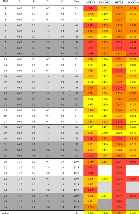
Table 1.Model runs of sensitivity study, their parameter combinations and the calculated misfit of tracers (J_RMSE) and OMZs (J_OMZ) for MIT2.8 and the ECCO1.0 configurations. The 25 % best simulations with regard toJ_RMSE andJ_OMZare highlighted in yellow and the worst 25 % in red (relative to RMSE^ECCO1.0^∗and OMZ^ECCO1.0^∗). The simulations in between are coloured in two orange gradations (bright orange is medium good and dark orange is medium bad). The best simulation of each resolution with regard toJ_RMSEandJ_OMZis bold.

OMZ is defined as 50 mmol m⁻³. Parameterηdenotes the exponent for size-dependent sinking,αthe stickiness,w₁the minimum sinking speed,DL the maximum diameter for size-dependent sinking and aggregation, andwmaxthe maximum sinking velocity in the spectral computations.

(5)

and Jackson, 2009; Jouandet et al., 2014). For the relationship between size and sinking speed we test two alternative values forη, namelyη=0.62 andη=1.17 for the exponent, andw₁between 0.7 and 2.8 m d⁻¹for the minimum sinking speed (see below). Assuming a constant degradation rate, the average sinking speed of all particles combined would increase with depth due to higher sinking speed of large particles and their higher proportion in the deeper ocean interior. To prevent instabilities at very large sinking speeds (very flat size distributions), as in Kriest and Evans (2000) and Kriest (2002), we restrict the size dependency of sinking and aggregation to a maximum diameter ofDL. BeyondDL, these processes do not vary with particle size any more. In our model experiments, we let this parameter vary between 1, 2 and 4 cm.

Changes in the number of marine particles are dependent on particle aggregation, described by the collision rate, and the probability that two particles stick together, α. In our model experiments we varyαbetween 0.2 and 0.8. The collision rate depends on turbulent shear and differential sinking and is parameterised as in Kriest (2002). We assume that the turbulent shear is high in the euphotic layers and 0 in the deeper ocean layers.

To avoid complications and non-linear feedbacks, in the experiments presented here, we assume that plankton mortality and zooplankton egestion as well as quadratic zooplankton mortality produce new detritus particles but do not change the size spectrum.

By using this setup, the module is similar to parameterisations of particle size applied in other large-scale or global models (Gehlen et al., 2006; Oschlies and Kähler, 2004;

Schwinger et al., 2016).

2.3 Model simulations and experiments 2.3.1 MOPS without aggregation

As a reference scenario, we used MOPS as described by Kriest and Oschlies (2015). The model has been imple- mented in both global configurations MIT2.8 (hereafter called noAgg^MIT2.8) and in the finer resolution, ECCO1.0 (noAgg^ECCO1.0).

2.3.2 Adjustment of biogeochemical model parameters Introducing aggregates and a dynamic particle flux profile to the global model MOPS has a strong impact on biogeochemical model dynamics. Starting from parameter values of the calibrated model setup (without aggregation) of Kri- est (2017), we calibrated parameters relevant for phytoplankton and zooplankton growth and turnover as described in Kri- est et al. (2017) against observed global distributions of nutrients and oxygen.

Parameters to be calibrated for this new model were the light and nutrient affinities of phytoplankton, zooplankton

quadratic mortality, detritus remineralisation rate, particle stickiness and the exponent η that relates particle sinking speed to particle size (see Table 2). After introduction of particle aggregation, the calibrated nutrient affinity of phytoplankton is now much higher, with a half-saturation constant for phosphate ofK_PHY=0.11 mmol PO₄m⁻³instead of 0.5 mmol PO₄m⁻³in Kriest et al. (2017), very likely because the optimisation compensates for the higher export (and lower recycling) of phosphorus and nitrogen. Possibly for the same reason, detritus remineralisation rate in the optimised model is increased from 0.05 to 0.25 d⁻¹. Light affinity of phytoplankton deviates less from the value in the model without particle aggregation, but the quadratic mortality of zooplankton is strongly reduced (1.6 (mmol P m⁻³)⁻¹ instead of 4.55 (mmol P m⁻³)⁻¹); the latter might be regarded as an attempt of the optimisation to reduce the export of organic matter from the euphotic zone. The two parameters that affect aggregation and particle sinking remained at moderate values of α=0.42 and η=0.72, i.e. close to those applied in earlier model experiments with aggregation (e.g.

Kriest, 2002). The residual cost functionJ_RMSEof this pre- calibrated model with aggregation was 0.472, i.e. lower than noAgg^MIT2.8 (J_RMSE=0.529), but somewhat higher than achieved with a model version optimised against nutrient and oxygen concentrations (Kriest et al., 2017), which resulted in a misfit ofJ_RMSE=0.439. In the sensitivity experiment described below we will examine whether this remaining misfit can be reduced even further and evaluate the model sensitivity to changes in the parameters of this highly complex module.

2.3.3 Sensitivity experiments at coarse resolution (MIT2.8)

In the coarser model configuration of MOPS, MIT2.8, a first sensitivity study of 36 model simulations with different aggregation parameters was performed (see Table 1). We varied the values of four aggregation parameters, which control the rate of aggregation and the sinking behaviour of particles.

The first parameter is the stickiness α, i.e. the probability that after collision two particles stick together, which was set to values of 0.2, 0.5 and 0.8, respectively. The second parameter is the maximum particle diameter for size-dependent aggregation and sinking,DL, set to values of 1, 2 and 4 cm.

A small value ofDLreduces the maximum possible sinking speed of the detrital pool and vice versa. Parameterw1de- scribes the sinking speed of a primary particle with values of 0.7, 1.4 and 2.8 m d⁻¹. One effect of a small value ofw1is that it reduces the loss of organic matter from surface layers, and thus it has a direct effect on the recycling of nutrients at the surface. At the same time, it also affects the maximum possible sinking speed of the entire detritus pool. Finally, the exponent that relates particle sinking to diameter,η, is set to values of either 0.62 and 1.17. A highηrepresents dense particles and a fast increase of particle sinking speed with size; a

(6)

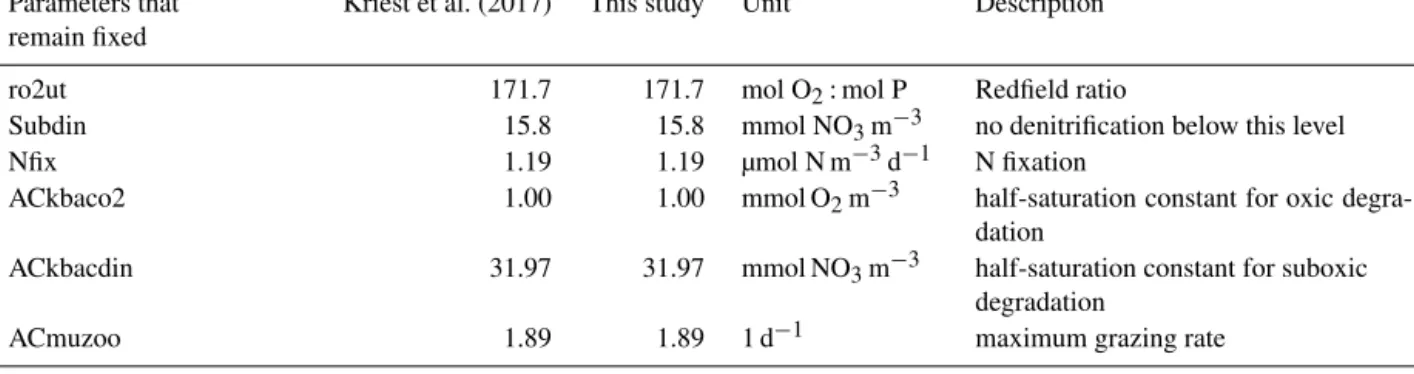
Table 2.Model adjustment of biogeochemistry with aggregates compared to Kriest et al. (2017) and new parameters in this study.

Parameters that Kriest et al. (2017) This study Unit Description remain fixed

ro2ut 171.7 171.7 mol O₂: mol P Redfield ratio

Subdin 15.8 15.8 mmol NO₃m⁻³ no denitrification below this level

Nfix 1.19 1.19 µmol N m⁻³d⁻¹ N fixation

ACkbaco2 1.00 1.00 mmol O₂m⁻³ half-saturation constant for oxic degra-

dation

ACkbacdin 31.97 31.97 mmol NO₃m⁻³ half-saturation constant for suboxic

degradation

ACmuzoo 1.89 1.89 1 d⁻¹ maximum grazing rate

Parameters that changed compared to Kriest et al. (2017)

ACik 9.65 6.52 W m⁻² light half-saturation constant

ACkpo4 0.5 0.106 mmol P m⁻³ half-saturation constant for PO₄uptake

AComniz 4.55 1.6 m³(mmol P d)⁻¹ quadratic zooplankton mortality

detlambda 0.05 0.25 1 d⁻¹ detritus remineralisation rate

New parameters for the aggregation model (further modified in this study)

SinkExp – 0.7164 exponent that relates particle sinking

speed to diameter

Stick – 0.4162 stickiness for interparticle collisions

low value stands for more porous particles, which show only a weak relationship between size and sinking speed (Kriest, 2002).

2.3.4 Sensitivity experiments at fine resolution (ECCO1.0)

The occurrence of aggregates, and their transport to the ocean interior, can furthermore depend on physical dynamics (e.g. Kiko et al., 2017). Therefore, in a second step, we repeated some of the experiments presented above in the finer-resolution version ECCO1.0 to investigate possible improvements at higher resolution. In particular, we repeated all MIT2.8 simulations withη=0.62 in this finer-resolution configuration. Additionally, we carried out three more simulations with η=1.17 but with the smallest DL=1 cm to prevent particles from sinking through more than one box per time step (see Table 1). All simulations together lead to 30 model runs in the finer-resolution configuration. To compare the ECCO1.0 simulations directly with results from MIT2.8, we re-gridded the result from ECCO1.0 simulations onto the coarser MIT2.8 grid.

2.4 Model assessment and diagnostics

Because observational data of particle flux are either limited with regard to space and time (e.g. Gehlen et al., 2006) or

are combined with assumptions that yield no clear patterns (Gehlen et al., 2006; Henson et al., 2012; McDonnell and Buesseler, 2010), this study restricts the model assessment to observations of nutrients and oxygen, in combination with the model fit to volume and location of oxygen minimum zones.

2.4.1 Root mean squared error of tracers

After a spinup of 3000 years into a seasonally cycling equi- librium state, the model results are evaluated in terms of annual means of oxygen, phosphate and nitrate. As in previous studies (e.g. Kriest et al., 2017) the misfit is calculated by the deviation between simulated results,m, and observed properties taken from the World Ocean Atlas (WOA),o(Garcia et al., 2006). The deviations are weighted by volume of each grid boxV_i, expressed as the fraction of the total ocean vol- umeV_T. The sum of the weighted deviations is normalised by the observed global mean concentration of each tracer:

J_RMSE=X3 j=1J (j )

=X3 j=1

1 o_j

s XN

i=1 mi,j−oi,j₂∗V_i

V_T. (1)

In this equation,j=1, 2, 3 describes the respective tracer (i.e. PO₄, NO₃ and O₂). N is the total number of model

(7)

grid boxes andoj is the global average observed concentration of each tracer (Kriest et al., 2017). Thus, a low misfit value represents a good agreement between model and observations (J_RMSE=0 would be a perfect fit), which enables a prediction about the model accuracy with regard to these tracers. The model runs with the lowestJ_RMSEin the coarse and the fine resolution are hereafter called RMSE^MIT2.8^∗and RMSE^ECCO1.0^∗, respectively.

2.4.2 Fit to oxygen minimum zones

To evaluate the extent and location of OMZs, we follow the approach of Cabré et al. (2015) by calculating the overlap between modelled and observed (Garcia et al., 2006; hereafter referred to as “WOA”) OMZs. As several marine processes are oxygen-dependent but have heterogeneous criteria for their minimum oxygen threshold, in this study, the OMZs are calculated for different oxygen threshold concentrations, C. Therefore, low-oxygen waters are characterised as O₂<c, withcranging from 0 to 100 mmol O₂m⁻³. To calculate the overlap between simulated and observed OMZs, we use the following equation (Sauerland et al., 2019):

C=V^∩(c)

V∪(c) = V^∩(c)

V^m(c)+V^o(c)−V^∩(c). (2) In this equation, V^∩(c)is the volume of overlap of suboxic waters between model and observations, with regard to the defined oxygen threshold concentration c. This overlap is divided by the union (total volume of low-oxygen waters occupied in the model or in the observations) and results in a value between 0, equal to zero overlap between model and observations, and 1, which represents an optimal overlap. To adjust the scale toJRMSE, we calculated the following:

JOMZ=1−C. (3)

In this equation, J_OMZ varies between 0 and 1. Conse- quently, the scale ofJ_OMZis equivalent to the scale ofJ_RMSE, which implies that a low misfit corresponds to a good agreement between model and observational data and vice versa.

The model simulations with regard to the lowest J_OMZ are called OMZ^MIT2.8^∗and OMZ^ECCO1.0^∗ hereafter. In calculating the overlap, we distinguish between the global ocean and the Pacific as well as the Atlantic Ocean.

2.4.3 Estimation of particle flux length scaleb

To investigate, if, and how, the model reproduced observed maps of the particle flux length scale, b, that relates particle flux and depth via F (z)∝z^−b and derived from data by Marsay et al. (2015) and Guidi et al. (2015), we log- transformedF (z), the simulated annual average flux of particulate organic matter as a function of depth, and carried out a linear regression of these values. The highestbvalues cor- respond to short particle flux length scale, i.e. many small

particles, and thus a low sinking speed, shallow remineralisation and high oxygen consumption in shallow waters. For the reference models without aggregation these global maps should, in areas with shallow mixed layers, show spatially uniform values, as imposed by the model’s prerequisites. De- viations from uniform values can be ascribed either to oxi- dant limitation of remineralisation (see above model description) or to physical processes such as mixing or upwelling, which can result in an additional vertical transport of particles.

The parameterisation of the aggregation model assumes a constant sinking speed for an upper size limitDL(see above), and therefore average particle sinking speed will remain constant below some depth. Also, the assumption of a particle size spectrum, size-dependent sinking and constant remineralisation will result in particle flux profiles that do not fully agree with those predicted by a power law (see Kriest and Oschlies, 2008). Thus, because the aggregation model’s prerequisites do not fully agree with a continuous increase of sinking speed with depth, we confine the regression of log- transformed particle flux to a vertical range between 100 and 1000 m, where the aggregation model still shows an increase of average sinking speed with depth (see also Kriest and Os- chlies, 2008).

3 Results

3.1 Global patterns of particle flux profiles

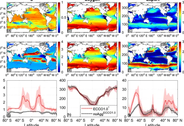
As could be expected, noAgg^ECCO1.0shows almost no spatial pattern of b, with values around the prescribed nominal value ofb=0.858 (global mean: 0.64; Fig. 1a; please note the different scaling in a and d) indicating long particle flux length scales and deep remineralisation. Regions with particularly low diagnosedbvalues (< 0.2) result either from decreased remineralisation in OMZs (e.g. eastern tropical Pacific OMZ) or are found in areas of deep mixing (in the model mainly high latitudes or western boundary currents), where vertical mixing increases the inferred particle flux length scales. However, for the best simulation with regard to the sum ofJRMSEandJOMZof the aggregation model (called ECCO1.0^∗ hereafter) we find the highest b values, corresponding to short particle flux length scales, or shallow remineralisation, in the oligotrophic subtropical gyres.

In contrast,bis the smallest in the equatorial upwelling and in the shelf regions (Fig. 1d and g). This pattern is in accor- dance with the observed spatial pattern derived by Marsay et al. (2015). In our model, this very deep flux penetration (b close to 0) in the equatorial upwelling can be explained with low oxygen concentrations, which reduce the remineralisation rate. In contrast, when deriving the particle flux length scale from a similar model but with oxygen-independent remineralisation (Kriest and Oschlies, 2013), we find a b

(8)

close to the prescribedbvalue of 0.858 (Fig. S1 in the Sup- plement).

In the subtropical and the equatorial region, the spatial variance (marked transparent red; Fig. 1g) of model-derived b values is quite high, which is caused by spatial variations in the physical environment, i.e. permanently stratified subtropical gyres and upwelling regions with low oxygen and reduced remineralisation. However, besides ECCO1.0^∗ the four best model simulations with respect to the sum of J_RMSEandJ_OMZ(simulation nos. 14, 17, 28 and 29; Table 1) show essentially the same pattern of b (Fig. S2), although these four simulations include quite different parameterisations (see Table 1).

Regions with high b values are characterised by a high spectral slope of the size distribution and therefore a high abundance of small particles, leading to slow sinking speeds (Fig. 7) and low export rates in ECCO1.0^∗ (Fig. 1f).

ECCO1.0^∗ simulates the highest export rates at high latitudes and in the upwelling region and the lowest export rates in the subtropical gyres (Fig. 1f and i). Although the spatial pattern of export rates is similar for both model simulations with and without aggregation, ECCO1.0^∗ shows a 1.6-fold higher global mean export rate (10.1 mmol P m⁻²a⁻¹) than noAgg^ECCO1.0 (6.1 mmol P m⁻²a⁻¹). In ECCO1.0^∗ export rates show a higher regional variability than in noAgg^ECCO1.0 (Fig. 1c, f and i), which is due to blooms in the high latitudes during summer season accelerating the size-dependent aggregation and thus the export signal.

The oxygen concentration at a depth of 100 m shows the same global pattern in both simulations, with high oxygen concentrations at high latitudes and decreasing concentrations towards the Equator (Fig. 1b and e). However, the oxygen concentration at high latitudes is slightly higher in noAggÊCCO1.0 than in ECCO1.0^∗ (Fig. 1h). Moreover, the global suboxic volume (for a criterionc=50 mmol m⁻³) in ECCO1.0^∗ (7.3×10¹⁶m³) is larger than in noAggÊCCO1.0 (3.7×10¹⁶m³). Comparing our model results with the dataset of Garcia et al. (2006), which yields a volume of 5.6×10¹⁶m³, we find an underestimation of the suboxic volume for noAggÊCCO1.0 by 34 % and an overestimation for ECCO1.0^∗by 30 %.

3.2 Representation of oxygen minimum zones

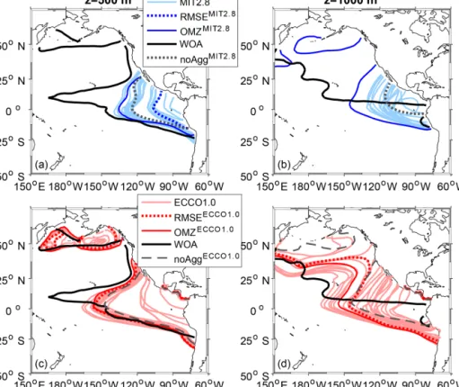
The finer-resolution and data-assimilated circulation of ECCO1.0 in general improves the representation of OMZs in comparison to MIT2.8 with regard to the overlap of OMZs for a criterion of 50 mmol m⁻³ (Fig. 2). Both simulations without explicit particle dynamics, namely noAgg^MIT2.8and noAgg^ECCO1.0, clearly underestimate the extent of the OMZ at a depth of 500 and 1000 m for an OMZ criterion of 50 mmol m⁻³in the Pacific basin (Fig. 2). The simulations including particle dynamics that are the best with respect to the OMZ metric, OMZ^MIT2.8^∗ and OMZ^ECCO1.0^∗, exhibit a larger OMZ area for both resolutions (Fig. 2). Despite the

improved representation of OMZs, all models including the particle aggregation module still tend to merge the OMZs of the Northern Hemisphere (NH) and the Southern Hemi- sphere (SH) at a depth of 500 m, which does not agree with the well-separated northern and southern OMZ shown by the observations (Figs. 2 and S3 in the Supplement). As reflected in a plot that shows the extent of OMZ in the NH and SH, similar to Fig. 1a and 1b of Cabré et al. (2015), all models fail to represent the double structure of OMZ north and south of the Equator. However, in our model the northern Pacific OMZ is fitted quite well (Figs. 2 and S3).

Aggregation improves the representation of OMZs with respect to a criterion of c=50 mmol m⁻³ compared to the simulations without aggregation for both resolutions in the NH, but not in the SH (Fig. 3). In noAggÊCCO1.0 the OMZ simulated in the NH is too small and too shallow (Fig. 3a). Even though OMZÊCCO1.0^∗ tends to underestimate the suboxic area between ∼700 and 1300 m, it shows a considerably higher overlap of model results and observations compared to noAggÊCCO1.0 (Fig. 3b). However, in the SH noAggÊCCO1.0 represents the OMZs better than OMZÊCCO1.0^∗, which tends to overestimate the suboxic area in this hemisphere. In addition to differences caused by particle dynamics, circulation affects the performance in the two hemispheres: OMZÊCCO1.0^∗ represents the highest overlap between∼100 and 500 m depth in the SH, but this is sur- passed by OMZ^MIT2.8^∗between 500 and 900 m depth. In the NH, OMZÊCCO1.0^∗ outcompetes OMZ^MIT2.8^∗ between 300 and 900 m depth as far as overlap is concerned (Fig. 3b).

However, the improvement of the representation of OMZs in the simulations with aggregation depends on the criterion for OMZs. As could be expected, a higher oxygen threshold for the OMZ criterion enhances the overlap between model simulations and observational data (Fig. 4). As for the fixed criterion of 50 mmol m⁻³, globally and in the Pacific the better circulation and finer resolution of ECCO1.0 improves the overlap for varying OMZ criteria in comparison to MIT2.8 (Fig. 4a and c). While the OMZ^ECCO1.0^∗ simulation reaches globally a maximum overlap of 65.9 % (for c=100 mmol m⁻³), OMZ^MIT2.8^∗culminates only in a maximum of 58.7 % for the same criterion.

In the Pacific basin OMZÊCCO1.0^∗ reaches an agreement with observations of 19.9 % overlap for a criterion of 20 mmol m⁻³(Fig. 4c). The overlap then increases strongly until the 100 mmol m⁻³ criterion (68.2 %). It is notewor- thy that globally and in the Pacific area noAggÊCCO1.0out- performs all models for a criterion of 20 mmol m⁻³, where it shows an agreement of almost 31 %. The Atlantic basin shows an inverse trend (Fig. 4b): here, OMZ^MIT2.8^∗ represents the OMZ better than OMZÊCCO1.0^∗(26 % and 12.2 %, respectively, for a criterion of 70 mmol m⁻³). Further, in this region, the ECCO1.0 model that performs best with respect to RMSE (RMSEÊCCO1.0^∗) outperforms OMZÊCCO1.0^∗ over the full range of criteria (Fig. 4b). Thus, there are large regional differences in the model’s response to different circu-

(9)

Figure 1.Global maps ofb(a, d), O₂at 100 m (mmol m⁻²,b, e) and export at 100 m (mmol P m⁻²a⁻¹,c, f) for noAgg^ECCO1.0(a, b, c) and for the best aggregation model with regard to the sum ofJ_RMSEandJ_OMZ(simulation no. 26;d, e, f). The black line indicates the OMZ for a criterion of 50 mmol m⁻³. Lower panels: Global mean (dotted line) and standard deviation (transparent shaded) ofb(g), O₂(h)and export(i)of noAgg^ECCO1.0(black) and the best aggregation model with regard to the sum ofJ_RMSEandJ_OMZ (simulation no. 26; red).

Please note the different scaling forbvalues(a, d).

Table 3.Number of simulations with different parameters forDL, αandw₁for the porous (η=0.62) and dense (η=1.17) particles which outperform the corresponding other size. The numbers are given with respect to two different criteria,J_RMSEandJ_OMZ.

η=0.62 η=1.17 Resolution

J_RMSE 6 3 MIT2.8

J_OMZ 8 1 MIT2.8

J_RMSE 2 1 ECCO1.0

J_OMZ 2 0 ECCO1.0

lations and particle dynamics. Because the dataset of observations used for comparison does not contain any concentrations below 30 mmol m⁻³in the Atlantic, all models show no overlap at all in this basin.

In summary, the improvement of model fit with regard to JOMZdepends not only on particle dynamics but also on the definition of OMZs (i.e. the OMZ criterionc), the model resolution as well as the region considered (Figs. 2, 3, 4).

3.3 Sensitivity of nutrient and oxygen distributions to aggregation parameters

Table 3 shows that in six cases out of nine (MIT2.8), a model that represents porous particles (η=0.62) outperforms the corresponding model with a sinking speed that describes rather dense, cell-like particles (η=1.17). The same applies for the higher resolution (ECCO1.0), where in two cases out of three a porous parameterisation improves the fit with regard toJ_RMSE(see Table 1). Also, bothJ_RMSEandJ_OMZof the “dense” parameterisations are never among the best five models with respect to either metric (see Table 1). Thus, in the following we focus on model simulations withη=0.62.

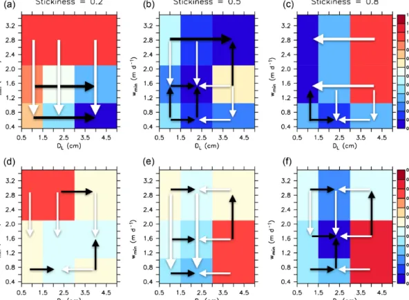
Among the sensitivity experiments performed, the best model with respect to JRMSE (hereafter referred to as RMSE^MIT2.8^∗) is characterised by an intermediate stickiness α of 0.5, the largest diameter for size-dependent aggregation and sinking,D_L, of 4 cm and a minimum particle sinking speed w₁ of 2.8 m d⁻¹, representing a rather fast organic matter transport to the ocean interior. However, many other models with medium stickiness perform about equally well (Fig. 5b). Models with lower stickiness perform best with slow minimum sinking speedw₁and a large maximum sizeD_L=4 cm for size-dependent sinking and aggregation

(10)

Figure 2.Comparison of Pacific Ocean OMZ (O₂≤50 mmol m⁻³) between model simulations and observations. Panels(a)and(b)show the OMZ at a depth of 500 and 1000 m for the coarse resolution, MIT2.8, and panels(c)and(d)for the fine resolution, ECCO1.0.

(Fig. 5a). In contrast, a large stickiness (which facilitates the formation of aggregates in surface layers) requires either smallw1orDL, which reduces the export of particles out of the euphotic zone, and into the ocean interior.

Oxygen concentrations contribute most to the global JRMSE (Kriest et al., 2017). The influence of oxygen on global tracer misfit is dominated by the deep concentrations (Fig. S4) and thus to a large extent by the large-scale circulation. The OMZs, because of their small regional extent, contribute less to the global misfit (Kriest et al., 2017). This is confirmed by Fig. S4d, e and f, showing that, in the eastern tropical Pacific region, deep (> 300 m) mesopelagic and deep oxygen concentrations scatter strongly among the different models (Fig. S4a), despite their good global match in shallow waters. Likewise, although global mean profiles of nutrients are quite similar among the different circulations, and agree quite well with observations, their concentrations scatter strongly in the eastern tropical Pacific. Most of the simulations tend to underestimate the oxygen and nitrate concentration in this region (Fig. S4a and c). Oxygen concentrations that are too low lead to denitrification that is too high and thus widespread nitrate depletion in the eastern tropical Pa- cific region, which explains the simultaneous underestimate of oxidants in this region.

To sum up, a moderate stickiness enhances the chance of a good model fit to nutrients and oxygen (J_RMSE), but there is

no unique trend for the parameters or combination of parameters, with the exception of the exponent that relates particle sinking speed to its size: here, we find an advantage of a parameterisation characteristic for porous marine aggregates.

In the optimal scenario, the misfit is less than that of a model without aggregates, when this is simulated with fixed reference parameters (noAgg^MIT2.8). Because of the small spatial extent of OMZs, the model fit to nutrient and oxygen concentrations is mainly caused by the large-scale tracer distribution, even if some models show a considerable mismatch to these tracers in OMZs.

The pattern for J_RMSE does not change very much when applying a different, more highly resolved and data- assimilated circulation (see Table 1 and Fig. 6). Now, the optimal model (RMSE^ECCO1.0^∗) is improved with respect to JRMSE by about 13 %, but many other almost equally good solutions can be found with moderate to high stickiness. Introducing aggregates in this coupled model system does not improve the model fit to nutrient and tracer concentrations, as evident from the comparison of RMSE^ECCO1.0^∗ (J_RMSE=0.431) against a model without aggregate dynamics (J_RMSE=0.426; Table 1). The lack of improvement can likely be explained by the fact that the biogeochemical parameters of MOPS with particle dynamics were adjusted in the circulation of MIT2.8, and thus they are not optimal

(11)

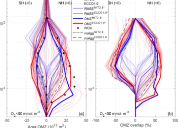
Figure 3. Area of OMZ (a) and overlap of OMZs between model and observations following Cabre et al. (2015)(b). In both panels, the left-hand side shows the Southern Hemisphere (0–

40^◦S); the right shows the Northern Hemisphere (0–40^◦N), plot- ted against the logarithmic depth. OMZs are defined as regions with O₂< 50 mmol m⁻³.

Figure 4.Overlap between modelled and observed OMZs (Eq. 2) for varying criteria c, ranging from 0<c<100 mmol m⁻³) on a global scale (a), for the Atlantic Ocean (b) and for the Pacific Ocean(c).

for the model when simulated in the physical dynamics of ECCO1.0.

The sensitivity to the metric for OMZs differs from the sensitivity to the metric for nutrients and oxygen. Now, for the fit to oxygen minimum zones (J_OMZ), a large stickiness (α), in combination withD_Lof 2 cm and slow-to-moderate minimum sinking speed w₁, is of advantage (Figs. 5 and 6). Thus, a high rate of aggregation, and a maximum sinking speed of about 50–100 m d⁻¹, improves the model with respect to OMZs. This is also evident from comparison

of the optimal models (OMZ^MIT2.8^∗ and OMZ^ECCO1.0^∗) to models without aggregate dynamics (noAgg^MIT2.8 and noAgg^ECCO1.0), shown in Figs. 3 and 4 and Sect. 3.2. Nev- ertheless, even the models that perform best with respect toJ_OMZunderestimate mesopelagic oxygen when averaged over the eastern tropical Pacific (Fig. S4a).

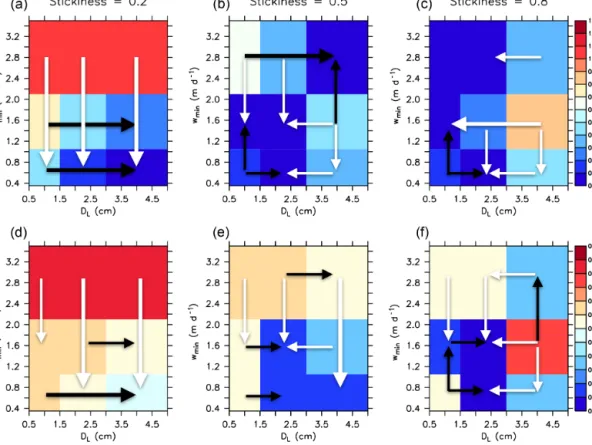
The sensitivity patterns with regard toJ_OMZ among both configurations MIT2.8 and ECCO1.0 diverge considerably from each other, which is in contrast to the patterns forJ_RMSE noted above (compare Fig. 5 with Fig. 6). Thus, model performance with respect toJ_OMZseems to depend much more on circulation and physical details than the large-scale dynamics reflected inJRMSE.

4 Discussion

In our sensitivity study, we used a similar parameterisation of particle aggregation as Oschlies and Kähler (2004) applied in their biogeochemical-circulation model for the North At- lantic Ocean. The difference compared to our model consists in aggregates, which are composed of phytoplankton and detritus, the parameterisation, which is based on dense particles (dSAM, Kriest, 2002) and a biogeochemical model, which is different. We found high values for the spectral slope of the size distribution (i.e. high abundance of small particles) and thus a low particle sinking speed in the subtropical gyres (Fig. 7), which corresponds with the findings by Oschlies and Kähler (2004) and Dutay et al. (2015). This, in turn, leads to the highestbvalues in the oligotrophic subtropical gyres and the lowest ones in the high latitudes and the upwelling region, in agreement with the pattern as shown in Marsay et al. (2015). These findings imply that such abpattern can result not only from temperature-dependent remineralisation – as suggested by Marsay et al. (2015) – but also from particle dynamics and temperature-independent remineralisation.

However, if temperature-dependent remineralisation, as suggested by Marsay et al. (2015) or Iversen and Ploug (2013), was also included in our model, this would likely enhance horizontal variations in the particle flux profile, with even deeper flux penetration in the cold waters of the high latitudes and upwelling areas. Besides particle dynamics, the lowb values in upwelling regions found in our study (Fig. 1d) are also caused by the suboxic conditions, which suppress remineralisation in subsurface waters. Such a tight link between suboxia and deep flux penetration is supported by the observations reported by Devol and Hartnett (2001) and Van Mooy et al. (2002). Therefore, two different processes – particle aggregation and/or temperature-dependent remineralisation – suggest lowb values and deep flux penetration in the very productive areas of high latitudes. A third process, which consists in oxygen-dependent remineralisation, is su- perimposed on these in OMZs, causing the steepest particle profiles in these areas.

(12)

Figure 5.Sensitivity ofJ_RMSE(Eq. 1);(a, b, c)andJ_OMZ(Eq. 3);(d, e, f)to minimum sinking speedw₁and maximum sizeD_Lfor the coarse resolution, MIT2.8, for three different values of stickiness(a–f), andη=0.62 (“porous” particles). The colour bar showsJ_RMSEand J_OMZ(blue – good fit, red – bad fit), normalised by its minimum value across all model experiments. Black arrows indicate an improvement ofJ_RMSEorJ_OMZwith increasing parameter values, while white arrows show an improvement with decreasing values.

However, it should be noted that although the maximum sinking speed of our best simulations (101 (no. 17) and 51 m d⁻¹(no. 26), see Table 1) agrees with observations (All- dredge and Gotschalk, 1988; Nowald et al., 2009; Jouandet et al., 2011), the range ofbvalues in our model is almost twice as large as suggested by most empirical studies (Berelson, 2001; Buesseler et al., 2007; Martin et al., 1987; Van Mooy et al., 2002). However, as there is no common depth range to determine the particle flux length scaleb, the depth range spreads over a wide range in various studies and thus im- pedes the comparability (Marsay et al., 2015), which might explain some divergence between observations and model results. In particular, our model simulates too large a fraction of small particles and therefore too steep a particle size spectrum in the subtropical gyres, which causesbvalues that are too high in these areas. Other processes that modify the size spectrum, like grazing by zooplankton, and the subsequent egestion of large fecal pellets, might also play a role in these regions. Additionally, the model tends to underestimate the number of large particles (size range 0.14 to 16.88 mm) in the surface of the tropical Atlantic Ocean (23^◦W), compared to observations (Kiko et al., 2017; Fig. S6). On the other hand, a first, direct comparison to the UVP 5 dataset (Kiko et al., 2017, their Fig. 1) exhibits a correct magnitude regarding the

number of particles within this size range (0.14 to 16.88 mm) in our model (Fig. S5) along the 151^◦W section. One possible explanation for the mismatch at 23^◦W could consist in a not sufficiently resolved equatorial current system, which also will be discussed below. Also, additional biological processes, such as the downward transport of organic matter through vertically migrating zooplankton (Kiko et al., 2017) or particle breakup of aged, fragile particles at depth (e.g.

Biddanda et al., 1988), could improve the model. However, introducing this additional complexity is beyond the scope of this paper. In future studies, consideration of these processes, in conjunction with a comprehensive model calibration against observed particle abundances and size spectra (e.g. Stemmann et al., 2002), may help not only to improve the representation of OMZs but also to better constrain the contributions of individual processes such as aggregation, vertical migration and temperature-dependent remineralisation, as well as to validate simulated particle dynamics.

However, model calibration against observed particle dynamics has to account for characteristics and limitations of observations. For example, the size spectrum assumed in our model is of infinite upper size and also contains particles with a diameter larger than, for example, 4 cm (the upper limit for size dependency of aggregation and sinking). While these

(13)

Figure 6.As Fig. 5 but for simulations with ECCO1.0.

Figure 7.Zonal mean sinking speed of detritus (m d⁻¹; dotted line) and its standard deviation (shaded) of ECCO1.0^∗ for a depth of 100 m(a)and for a depth of 500 m(b).

particles exist (e.g. Bochdansky and Herndl, 1992), they are very rare (in the model, and likely also in the observations) and might not be observed with standard methods, which usually rely on a sample size of a few litres. The rare occurrence of large particles (and the limited sample size) has, for example, consequences for estimated size spectra parameters

(Blanco et al., 1994). Thus, any model calibration against observations of particle abundance and size has to account for a proper match between simulated and observed quantities.

As we used on the one hand two different model grid resolutions and on the other hand varied model parameterisations with regard to particle aggregation, changes in the location and extension of OMZs and the distribution of tracers within each resolution are exclusively driven by the aggregation parameters. A good parameterisation of particle aggregation parameters can therefore have a major influence on the representation of OMZs. Furthermore, a higher model resolution improves the depiction of equatorial currents and therefore the oxygen transport (Cabré et al., 2015; Duteil et al., 2014), which, in turn, results in an improved representation of OMZs in the finer-resolution configuration, ECCO1.0, compared to the coarser resolution, MIT2.8. How- ever, as physical processes at smaller scales affect the simulated shallow to mesopelagic oxygen and nutrient concentrations for the eastern tropical Pacific (Getzlaff and Dietze, 2013), the finer (1^◦×1^◦) resolution of ECCO1.0 is not sufficient to resolve the details of the equatorial current system (Duteil et al., 2014). This can explain the still high residual misfit of these simulations and the missing double structure of OMZs in the eastern tropical Pacific. We therefore suggest that the difference in improving the representation of OMZs between NH and SH is more affected by physics than by bi- ology.

(14)

Furthermore, the results of our sensitivity study confirm that dense particles do not constitute a realistic representation of particles, as indicated by Karaka¸s et al. (2009) and Kriest (2002). Porous particles seem to constitute a more appropriate parameterisation for good model fit with regard to J_RMSEandJ_OMZ(Table 1). Although the observed stickiness ranges between almost 0 and 1 (e.g. Alldredge and McGilli- vary, 1991; Kiørboe et al., 1990), in our study a moderate stickiness,α, between 0.5 and 0.8 leads the model towards a good fit to observed nutrients, oxygen and OMZs.

In summary, our study supports the results of Schwinger et al. (2016), who found an improved representation of nutrient distribution and OMZs when switching from constant particle sinking to either a power law or particle dynamics, similar to those presented here. However, the difference between the two latter schemes in that study were only small. A more extensive search of the parameter space within a given circulation may further improve the model. Additionally, we optimised noAgg^MIT2.8 against the same misfit function as MOPS^oDof Kriest et al. (2017) and found that even though including an aggregation module improves our model, util- ising an appropriate parameter optimisation would further enhance our model fit. Thus, without a comprehensive calibration of biogeochemical and aggregation parameters, there only seems to be a slight advantage when using this more complex model of particle dynamics.

Finally, we found a steep particle size spectrum in the subtropical oligotrophic region (Fig. 1d), which does not agree with observational data. Potentially, there are processes tak- ing place that are not considered in our model, i.e. particle repackaging and active transport by zooplankton (vertical migration) (Kiko et al., 2017) based on a modified food web.

Thus, particle aggregation alone so far seems not to be sufficient for a correct representation of the particle size spectrum.

5 Conclusion and outlook

Najjar et al (2007) applied different model circulations to the same biogeochemical model and found that physical processes are an important factor for modelling marine biogeochemistry. Our study furthermore showed that also biogeochemical parameterisations – in particular, those related to particle flux – can have an important impact on the representation of dissolved inorganic tracers, in line with earlier studies (e.g. Kriest et al., 2012; Kwon and Primeau, 2006, 2008). These earlier studies applied and varied a globally uniform particle flux length scale, whereas it has been suggested that this parameter should vary in space and time (e.g.

Guidi et al., 2015; Marsay et al., 2015). The sensitivity study presented here constitutes a first approach to systematically estimate the impact of marine particle aggregation – and thus a spatially and temporally variable flux length scale – on the location and extent of OMZs as well as the representation of

phosphate, nitrate and oxygen under steady-state conditions in a global three-dimensional biogeochemical ocean model.

We have shown that the assumptions inherent in the model confirm the general pattern of the spatial map ofbvalues proposed by Marsay et al. (2015) (Fig. 1a and d). This, in turn, shows that the pattern of Martin’sbcan be depicted not only by a particulate organic carbon flux dependent on temperature but also by simulating explicit particle dynamics.

We furthermore found that even though there are still a lot of gaps in understanding several processes (e.g. the variation of export rates, particle stickiness and particle flux profile over space and time, as well as the link between particle diameter and sinking speed), the comparisons against observational data show a trend towards a model improvement by integrating particle dynamics (Table 1). While the parameterisation of aggregation leads the model towards an improved fit to OMZs for both model resolutions, this increase in model fit with regard to phosphate, nitrate and oxygen is only detectable in the coarse-resolution MIT2.8, but not in the finer-resolution and data-assimilated circulation of ECCO1.0. Moreover, model simulations show that besides effects of grid resolution, the model fit with regard toJ_RMSE andJ_OMZis mainly driven by the particles’ porosity. Our results indicate that a best fit to both tracers as well as OMZs (50 mmol O₂m⁻³ criterion) is achieved by parameterising porous particles in combination with an intermediate-to-large maximum particle diameter for size-dependent aggregation and sinking, a moderate-to-high stickiness ranging between 0.5 and 0.8, and an intermediate-to-high initial sinking speed ranging between 1.4 and 2.8 m d⁻¹(Fig. 5). The strong sensitivity of the model fit to aggregation parameters may point towards the importance of a spatially and temporally varying flux length scale; however, they also show that the dynamics of the model depend strongly on the assumptions we make with respect to particle properties and processes.

Finally, we have shown that uncertainties in the parameterisation of particle aggregation remain, leading to the in- ference that dissolved inorganic tracers offer only insuffi- cient observational constraints for global particle parameterisation. Therefore, for an accurate representation it will be necessary to calibrate the model not only against observed phosphate, nitrate, oxygen distributions and volume and location of OMZs (Sauerland et al., 2019) but also against number and size of particles, using comprehensive datasets of observations (as in Guidi et al., 2015).

Code and data availability. The source code of MOPS including the aggregation module coupled to TMM as well as the model out- put are available at: https://data.geomar.de/thredds/catalog/open_

access/niemeyer_et_al_2019_bg/catalog.html (Niemeyer, 2019).

The source code of the TMM is available at: https://github.com/

samarkhatiwala/tmm (Khatiwala, 2019).

(15)

Supplement. The supplement related to this article is available on- line at: https://doi.org/10.5194/bg-16-3095-2019-supplement.

Author contributions. DN, IK and AO conceived the study. DN performed and analysed the simulations. All authors discussed and wrote the manuscript.

Competing interests. The authors declare that they have no conflict of interest.

Acknowledgements. This work is a contribution to DFG-supported project SFB 754 (https://www.sfb754.de, last access: 13 Au- gust 2019). Parallel supercomputing resources have been provided by the North-German Supercomputing Alliance (HLRN) and the computing centre at Kiel University. We thank two anonymous re- viewers for their helpful comments.

Financial support. The article processing charges for this open- access publication were covered by a Research Centre of the Helmholtz Association.

Review statement. This paper was edited by Fortunat Joos and re- viewed by two anonymous referees.

References

Alldredge, A. L. and Gotschalk, C.: In situ settling behavior of marine snow, Limnol. Ocean., 33, 339–351, 1988.

Alldredge, A. L. and McGillivary, P.: The attachment probabil- ities of marine snow and their implications for particle co- agulation in the ocean, Deep-Sea Res. Pt. A, 38, 431–443, https://doi.org/10.1016/0198-0149(91)90045-H, 1991.

Armstrong, R. A., Lee, C., Hedges, J. I., Honjo, S., and Wake- ham, S. G.: A new, mechanistic model for organic carbon fluxes in the ocean based on the quantitative association of POC with ballast minerals, Deep-Sea Res. Pt. II, 49, 219–236, https://doi.org/10.1016/S0967-0645(01)00101-1, 2002.

Banse, K.: New views on the degradation and disposition of organic particles as collected by sediment traps in the open sea, Deep- Sea Res. Pt. A, 37, 1177–1195, https://doi.org/10.1016/0198- 0149(90)90058-4, 1990.

Berelson, W.: The flux of particulate organic carbon into the ocean interior, Oceanography, 14, 59–67, https://doi.org/10.5670/oceanog.2001.07, 2001.

Berelson, W. M.: Particle settling rates increase with depth in the ocean, Deep-Sea Res. Pt. II, 49, 237–251, https://doi.org/10.1016/S0967-0645(01)00102-3, 2002.

Biddanda, B. A. and Pomeroy, L. R.: Microbial aggregation and degradation of pyhtoplankton-derived detritus in seawater, I. Mi- crobial succession, Mar. Ecol. Prog. Ser., 42, 79–88, 1988.

Blanco, J. M., Echevarria, F., and Garcia, C. M.: Dealing with size- spectra: Some conceptual and mathematical problems, Sci. Mar., 58, 17–29, 1994.

Bochdansky, A. B. and Herndl, G. J.: Ecology of amorphous ag- gregations (marine snow) in the Northern Adriatic Sea, III. Zoo- plankton interactions with marine snow, Mar. Ecol. Prog. Ser., 87, 135–146, 1992.

Boyd, P. W. and Trull, T. W.: Understanding the export of biogenic particles in oceanic waters: Is there consensus?, Prog. Oceanogr., 72, 276–312, https://doi.org/10.1016/j.pocean.2006.10.007, 2007.

Buesseler, K. O., Lamborg, C. H., Boyd, P. W., Lam, P. J., Trull, T.

W., Bidigare, R. R., Bishop, J. K. B., Casciotti, K. L., Dehairs, F., Elskens, M., Honda, M., Karl, D. M., Siegel, D. A., Silver, M. W., Steinberg, D. K., Valdes, J., Mooy, B. Van, and Wilson, S.: Revis- iting Carbon Flux Through the Ocean’s Twilight Zone, Science, 316, 567–570, https://doi.org/10.1126/science.1137959, 2007.

Burd, A. B.: Modeling particle aggregation using size class and size spectrum approaches, J. Geophys. Res.-Ocean., 118, 3431–3443, https://doi.org/10.1002/jgrc.20255, 2013.

Burd, A. B. and Jackson, G. A.: Particle aggregation, Annu. Rev. Mar. Sci., 1, 65–90, https://doi.org/10.1146/annurev.marine.010908.163904, 2009.

Cabré, A., Marinov, I., Bernardello, R., and Bianchi, D.: Oxy- gen minimum zones in the tropical Pacific across CMIP5 models: Mean state differences and climate change trends, Biogeo- sciences, 12, 5429–5454, https://doi.org/10.5194/bg-12-5429- 2015, 2015.

Cocco, V., Joos, F., Steinacher, M., Frölicher, T. L., Bopp, L., Dunne, J., Gehlen, M., Heinze, C., Orr, J., Oschlies, A., Schneider, B., Segschneider, J., and Tjiputra, J.: Oxy- gen and indicators of stress for marine life in multi-model global warming projections, Biogeosciences, 10, 1849–1868, https://doi.org/10.5194/bg-10-1849-2013, 2013.

Devol, A. H. and Hartnett, H. E.: Role of the oxygen-deficient zone in transfer of organic carbon to the deep ocean, Limnol. Ocean., 46, 1684–1690, https://doi.org/10.4319/lo.2001.46.7.1684, 2001.

Dutay, J. C., Tagliabue, A., Kriest, I., and van Hulten, M. M.

P.: Modelling the role of marine particle on large scale 231Pa, 230Th, Iron and Aluminium distributions, Prog. Oceanogr., 133, 66–72, https://doi.org/10.1016/j.pocean.2015.01.010, 2015.

Duteil, O., Böning, C. W., and Oschlies, A.: Variability in subtropical-tropical cells drives oxygen levels in the tropical Pacific Ocean, Geophys. Res. Lett., 41, 8926–8934, https://doi.org/10.1002/2014GL061774, 2014.

Engel, A. and Schartau, M.: Influence of transparent ex- opolymer particles (TEP) on sinking velocity of Nitzschia closterium aggregates, Mar. Ecol. Prog. Ser., 182, 69–76, https://doi.org/10.3354/meps182069, 1999.

Garcia, H. E., Locarnini, R. A., Boyer, T. P., and Antonov, J. I.:

World Ocean Atlas 2005, Volume 3: Dissolved Oxygen, Appar- ent Oxygen Utilization, and Oxygen Saturation, edited by: Levi- tus, S., NOAA Atlas NESDIS 63, US Gov. Print. Off. Washing- ton, DC, 3, 342 pp., 2006.

Gehlen, M., Bopp, L., Emprin, N., Aumont, O., Heinze, C., and Ragueneau, O.: Reconciling surface ocean productiv- ity, export fluxes and sediment composition in a global