A model study of warming-induced phosphorus–oxygen feedbacks in open-ocean oxygen minimum zones

(1)

www.earth-syst-dynam.net/8/357/2017/

doi:10.5194/esd-8-357-2017

A model study of warming-induced phosphorus–oxygen feedbacks in open-ocean oxygen minimum zones

on millennial timescales

Daniela Niemeyer¹, Tronje P. Kemena¹, Katrin J. Meissner², and Andreas Oschlies¹

1Helmholtz-Zentrum für Ozeanforschung Kiel (GEOMAR), Düsternbrooker Weg 20, 24105 Kiel, Germany

2Climate Change Research Centre and ARC Centre of Excellence for Climate System Science, University of New South Wales, Level 4 Mathews Building, Sydney, New South Wales, 2052, Australia

Correspondence to:Daniela Niemeyer (dniemeyer@geomar.de) Received: 20 October 2016 – Discussion started: 31 October 2016 Revised: 20 March 2017 – Accepted: 12 April 2017 – Published: 19 May 2017

Abstract. Observations indicate an expansion of oxygen minimum zones (OMZs) over the past 50 years, likely related to ongoing deoxygenation caused by reduced oxygen solubility, changes in stratification and circulation, and a potential acceleration of organic matter turnover in a warming climate. The overall area of ocean sediments that are in direct contact with low-oxygen bottom waters also increases with expanding OMZs. This leads to a release of phosphorus from ocean sediments. If anthropogenic carbon dioxide emissions continue unabated, higher temperatures will cause enhanced weathering on land, which, in turn, will increase the phosphorus and alkalinity fluxes into the ocean and therefore raise the ocean’s phosphorus inventory even further. A higher availability of phosphorus enhances biological production, remineralisation and oxygen consumption, and might therefore lead to further expansions of OMZs, representing a positive feedback. A negative feedback arises from the enhanced productivity-induced drawdown of carbon and also increased uptake of CO2due to weathering-induced alkalinity input. This feedback leads to a decrease in atmospheric CO2and weathering rates. Here, we quantify these two competing feedbacks on millennial timescales for a high CO₂emission scenario. Using the University of Victoria (UVic) Earth System Climate Model of intermediate complexity, our model results suggest that the positive benthic phosphorus release feedback has only a minor impact on the size of OMZs in the next 1000 years.

The increase in the marine phosphorus inventory under assumed business-as-usual global warming conditions originates, on millennial timescales, almost exclusively (> 80 %) from the input via terrestrial weathering and causes a 4- to 5-fold expansion of the suboxic water volume in the model.

1 Introduction

Oxygen minimum zones (OMZs) have more than quadru- pled over the past 50 years and it has been suggested that this expansion is related to recent climate change (Stramma et al., 2008; Schmidtko et al., 2017). However, current CO₂ emission-forced models are challenged to reproduce this expansion in detail (Stramma et al., 2012; Cabré et al., 2015).

There are at least three different processes that can have an impact on the size of OMZs in a warming climate: ocean warming and its impact on solubility of O₂ in the ocean (Bopp et al., 2002), changes in ocean dynamics, e.g. strat-

ification, convective mixing and circulation (Manabe and Stouffer, 1993; Sarmiento et al., 1998), biological production effects (Bopp et al., 2002) including possible CO₂-driven changes in stoichiometry (Oschlies et al., 2008) and CO₂- induced changes in ballasting particle export (Hofmann and Schellnhuber, 2010). Here, we investigate how changes in biological production and subsequent remineralisation can af- fect OMZs in addition to the above-mentioned thermal and dynamic effects. We focus on changes in the phosphorus (P) cycle. P is the main limiting nutrient on long timescales (Tyrell, 1999; Palastanga et al., 2011) and we examine possible effects of changes in the P cycle on millennial timescales.

(2)

The major source of P for the ocean is river input (Fil- ippelli, 2008; Payton and McLoughlin, 2007; Föllmi, 1996;

Palastanga et al., 2011; Froelich et al., 1982), which is deter- mined by terrestrial weathering of apatite (Filippelli, 2002;

Föllmi, 1996). The main factors controlling terrestrial weathering are temperature, precipitation and vegetation. Higher temperatures are generally associated with enhanced precipitation and occur in many places with higher terrestrial net primary productivity (Monteiro et al., 2012), which all tend to increase weathering rates (Berner, 1991).

It is difficult to determine how much of the globally weath- ered P enters the ocean in a bioavailable form. Today, about 0.09–0.15 Tmol a⁻¹ of prehuman, potentially bioavailable P is transported globally by rivers including dissolved organic and inorganic P, particulate organic P and iron-bound P (Compton et al., 2000). About 25 % of this potentially bioavailable P is trapped in coastal estuaries and will not en- ter the open ocean (Compton et al., 2000). Ruttenberg (2004) estimated a bioavailable P flux under pre-industrial conditions including dissolved P and bioavailable particulate P (35 % of total particulate P) of 0.24–0.29 Tmol P a⁻¹exclud- ing the atmospheric input (Ruttenberg, 2004). Marine organisms take up P most easily as dissolved inorganic P (DIP).

Riverine measurements suggest that only a small fraction of the total P (0.012 to 0.032 Tmol a⁻¹) enters the ocean as DIP (Filippelli, 2002; Harrison et al., 2005; Compton et al., 2000;

Wallmann, 2010; Palastanga et al., 2011; Ruttenberg, 2004).

However, passing through estuaries can increase the fraction of DIP by 50 % (Froelich, 1984) to 80 % (Berner and Rao, 1994).

After taking up the bioavailable P for photosynthetic production of biomass, a large fraction of the newly produced organic matter is exported out of the euphotic zone as detritus (6.42 Tmol P a⁻¹, according to the model study by Palas- tanga et al., 2011) and the vast majority of this exported organic matter is remineralised in the deeper ocean by bac- teria (6.26 Tmol P a⁻¹; Palastanga et al., 2011), which is an oxygen consuming process. A small fraction of the exported organic matter is deposited at the sediment surface (0.16 Tmol P a⁻¹; Palastanga et al., 2011), about 20 % of the deposited P is buried in the sediments on long timescales (0.032 Tmol P a⁻¹; Palastanga et al., 2011) and the remaining 80 % (0.13 Tmol P a⁻¹; Palastanga et al., 2011) is released back into the water column as DIP, where it is again available for the uptake of marine primary producers (Palastanga et al., 2011; Wallmann, 2010).

The processes of burial and release of P are redox dependent. Under oxic conditions the burial rate is high, while under suboxic conditions the benthic release of P is elevated (Ingall and Jahnke, 1994; Kraal et al., 2012; Wallmann, 2010;

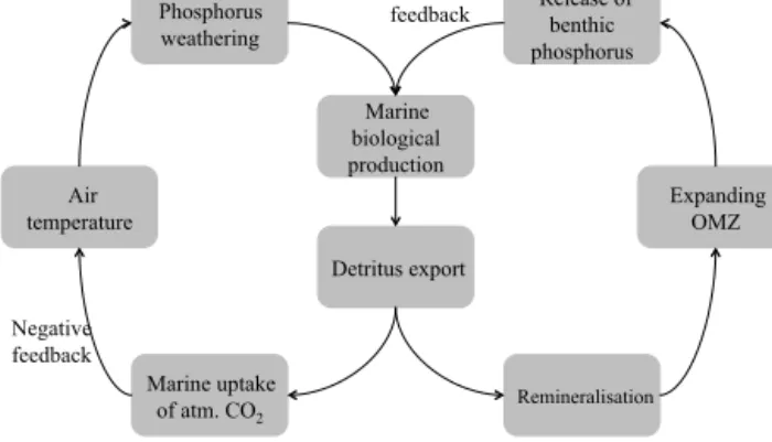
Slomp and Van Cappellen, 2007; Floegel et al., 2011; Lenton and Watson, 2000; Tsandev and Slomp, 2009). The redox- dependent release of P into the water column and the decrease in marine oxygen due to remineralisation therefore represent a positive feedback loop on marine biological pro-

Marine biological production

Detritus export

Marine uptake of atm. CO₂ Air

temperature

Phosphorus weathering

Release of benthic phosphorus

Expanding OMZ

Remineralisation Positive

feedback

Negative feedback

Figure 1.Possible feedbacks in the global phosphorus cycle under climate warming conditions.

duction (see Fig. 1). Although the feedbacks between ocean and atmosphere are complex (Sabine et al., 2004), we as- sume that an enhanced detritus export into the ocean interior results in an increased marine uptake of atmospheric CO2

(Sarmiento and Orr, 1991). Consequently, surface air temperatures decrease with decreasing atmospheric CO2concen- trations, which, in turn, leads to lower weathering rates (see Fig. 1).

These redox-dependent benthic P fluxes have been investigated in a previous study with the HAMOCC global ocean biogeochemistry model by Palastanga et al. (2011). Palas- tanga et al. (2011) show that doubling the input of dissolved P from rivers results in an increased benthic release of P.

This leads to a rise in primary production as well as in oxygen consumption, which in turn affects the oxygen availability in sediments. The benthic release of P acts therefore as a positive feedback on expanding oxygen minimum zones on timescales of 10 000 to 100 000 years (Palastanga et al., 2011).

Other studies on marine oxygen deficiency focused on the geological past, especially the mid-Cretaceous warm pe- riod (120–80 Ma) (Tsandev and Slomp, 2009; Handoh and Lenton, 2003; Bjerrum et al., 2006; Föllmi et al., 1996). Sev- eral periods of oceanic oxygen depletion have been inferred from sediment data of black shales (Schlanger and Jenkyns, 1976), for example, for the Cretaceous oceanic anoxic event 2 (OAE) at the Cenomanian–Turonian boundary (93.5 Myr).

Whether processes such as surface warming, sea-level rise (Handoh and Lenton, 2003), and possibly a slow-down of the ocean overturning circulation and vertical mixing (Monteiro et al., 2012; Tsandev and Slomp, 2009; Ruvalcaba Baroni et al., 2014) – as assumed for the Cretaceous – will lead to widespread oxygen depletion in the future is a reason of con- cern. Consequently, a better understanding of biogeochemical processes associated with Cretaceous OAE might help assess the risk of possible future events of low marine oxygen concentrations (Tsandev and Slomp, 2009).

(3)

In contrast to previous studies that focus on the geological past, we investigate possible future changes over the next 1000 years using an Earth System Climate Model of intermediate complexity to investigate the feedbacks between the P cycle and OMZs under the extended Representative Concen- tration Pathways Scenario 8.5 (RCP8.5) of the Intergovern- mental Panel on Climate Change (IPCC) AR5 report. The RCP8.5 scenario is characterised by an increase in atmospheric CO₂concentrations and associated with an increase in radiative forcing of up to 8.5 W m⁻²by year 2100 (in comparison to pre-industrial conditions) and is also known as the

“business as usual” scenario (Riahi et al., 2011).

2 Methods

2.1 UVic model

The University of Victoria Earth System Climate model (UVic ESCM) version 2.9 (Weaver et al., 2001; Eby et al., 2009) is a model of intermediate complexity and consists of a terrestrial model based on TRIFFID and MOSES (Meissner et al., 2003) including weathering (Meissner et al., 2012), an atmospheric energy–moisture balance model (Fan- ning and Weaver, 1996), a CaCO₃-sediment model (Archer, 1996), a sea-ice model (Semtner, 1976; Hibler, 1979; Hunke and Dukowicz, 1997) and a three-dimensional ocean circulation model (MOM2) (Pacanowski, 1995). The ocean model includes a marine ecosystem model based on a nutrient–

phytoplankton–zooplankton–detritus model (Keller et al., 2012). The horizontal resolution of all model components is 1.8^◦latitude×3.6^◦longitude. The ocean model has 19 layers with layer thicknesses ranging from 50 m at the sea surface to 500 m in the deep ocean. We use a sub-grid-scale bathymetry as described in Somes et al. (2013) to simulate benthic fluxes of phosphorus. The sub-grid bathymetry is inferred from the ETOPO2v2¹ and represents global spatial distributions of continental shelves, slopes and other topographical features (1/5^◦). For the topography used here, the shelf (0–200 m) covers 6.5 %, the slope (200–2000 m) 11.7 % and the deep sea (> 2000 m) 81.9 % of the global ocean. Downward fluxes of organic matter are intercepted by the sub-grid bathymetry related to the fractional sediment cover for each ocean grid box, and benthic fluxes of phosphorus are calculated based on the transfer functions described in the following section.

2.2 Phosphorus cycle in UVic model

Earlier applications of the UVic ESCM assumed a fixed marine P inventory. We included a representation of the dynamic P cycle for this study. It consists of a modified terrestrial weathering module (Meissner et al., 2012) and a redox- sensitive transfer function for burial and benthic release of P (Floegel et al., 2011; Wallmann, 2010).

1https://www.ngdc.noaa.gov/mgg/global/etopo2.html

The continental weathering module developed earlier for fluxes of dissolved inorganic carbon (DIC) and alkalinity (Meissner et al., 2012; Lenton and Britton, 2006) is based on the following equations:

FDIC,w=FDIC,w,0·

fSi+fCa· NPP

NPP₀

(1)

·(1+0.087·(SAT−SAT₀))

=F_DIC,w,0·f(NPP,SAT) F_Alk,w=F_Alk,w,0·

NPP NPP₀

·

f_Si·(1+0.038) (2)

·(SAT−SAT₀)·0.65^0.09·(SAT−SAT₀)k +f_Ca·(1+0.087·(SAT−SAT₀)),

whereFDIC,w andFAlk,w represent the globally integrated flux of DIC and alkalinity via river runoff;fSiandfCastand for the fraction of silicate (0.25) and carbonate (0.75) weathering; and NPP and SAT are the global mean net primary production on land and global mean surface air temperature over land (in degrees Celsius). The index 0 stands for pre- industrial values.

We added the following flux to account for P weathering (F_DP,w) with the same dependencies on globally and annu- ally averaged net primary production (NPP) and surface air temperature (SAT) as those for DIC:

FDP,w=FDP,0·f(NPP,SAT). (3)

The global river input of DIP is the only continental source for P in the model. The global DIP input is distributed over all coastal points of discharge scaled according to their indi- vidual volume discharge. The pre-industrial DIP input to the ocean (FDP,0) is assumed to be in steady state and in equilibrium with the total globally integrated pre-industrial net burial of P (BUR_P):

F_DP,0=BUR_P,0. (4)

We use an empirical transfer function for BUR_P and for the benthic release of DIP (BEN_DIP) derived from observations across bottom-water oxygen gradients (Wallmann, 2010; Flögel et al., 2011). The release of dissolved inorganic P (BEN_DIP) is calculated as follows:

BEN_DIP=BEN_DIC rreg

. (5)

Benthic release of dissolved inorganic carbon (BEN_DIC) is calculated from an empirical transfer function (Fig. 2 in Flögel et al., 2011) to determine BEN_DIP fluxes at the bottom of the ocean. In our model configuration, particulate organic carbon (POC) is remineralised completely at the ocean bottom and no ocean-to-sediment fluxes of POCs occur, i.e.

BEN_DICis equivalent to RR_POC, where RR_POCdenotes the

(4)

1800 2000 2200 2400 2600 2800 3000 2

2.5 3

Time [years]

PO4 [mmol P m−3]

(b)

1800 2000 2200 2400 2600 2800 3000 5 10

Export [Tmol P a−1]

REF PO₄ WB PO₄ REF exp.

WB exp.

1800 2000 2200 2400 2600 2800 3000

−0.2 0 0.2 0.4 0.6 0.8

Time [years]

P−fluxes [Tmol P a]−1

(c)

WB release WB weath.

1800 2000 2200 2400 2600 2800 3000 0

2 4 6 8x 10⁷

Time [years]

Suboxic volume [km]3

(d)

1800 2000 2200 2400 2600 2800 30000 2 4 6 x 108 ⁶

Suboxic sediment water [km2]

REF vol.

WB vol.

REF sed.

WB sed.

1800 2000 2200 2400 2600 2800 3000 12

14 16 18 20 22 24

SAT [oC]

0 500 1000 1500 2000 2500

CO−concentration [ppm]2

1800 2000 2200 2400 2600 2800 30000 20 40 60 80 100 120

Time [years]

(a)

CO−emit [Pg CO a]22−1

REF SAT WB SAT REF emit WB emit REF conc.

WB conc.

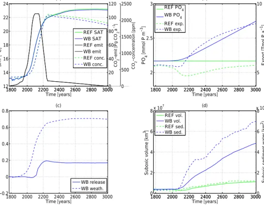
Figure 2.Global and annual mean time series of(a)surface air temperature in degree Celsius (solid lines), CO₂emissions in Pg CO₂a⁻¹ (black solid line – for both simulations) and CO₂ concentration in ppm (dashed lines);(b) global mean phosphorus concentration in mmol P m⁻³(solid lines) and export rate in Tmol P a⁻¹at 130 m depth (dashed lines);(c)anomalies of phosphorus input via sediment in Tmol P a⁻¹(solid line) and anomalies of phosphorus weathering input in Tmol P a⁻¹(dashed line);(d)suboxic volume (< 0.005 mol m⁻³) of the ocean in km³(solid lines) and surface of ocean bottom layer with O₂concentrations below 0.005 mol m⁻³in km²(dashed lines). The control simulation (REF) is shown in green; the second simulation (WB) is in blue.

rain rate of particulate organic carbon to the sediment. Wall- mann (2010) calculatedrregby a regression of observational data to bottom-water oxygen concentrations:

r_reg= RR_POC BENDIP

=Y_F+A·exp

−[O₂] r

. (6)

The regeneration ratio is calculated by dividing the depth- integrated rate of organic matter degradation in surface sediments (RRPOC) by the benthic flux of dissolved inorganic P into the bottom water (BENDIP). Parameters are defined as YF =123±24,A= −112±24 andr=32±19, and O2 is in µmol L⁻¹(Wallmann, 2010). Under oxic conditions r_regis higher than the Redfield ratio (106; Redfield et al., 1963) and under oxygen-depleted conditionsr_reg reduces to 10 (Wall- mann, 2010).

The rain rate of POP (RR_POP) is calculated by the rain rate of POC (RR_POC) divided by the Redfield ratio. As a result BUR_P can be calculated as follows:

BUR_P=RR_POP−BEN_DIP. (7)

The burial of P (BUR_P) in the sediment is equal to the rain rate of particulate organic P (RR_POP) minus BEN_DIP(Floegel

et al., 2011). If the benthic release overcomes the rain rate of POP at depths below 1000 m, the burial is set to zero. Follow- ing Floegel et al. (2011), this condition is not applied to shal- lower sediments because these deposits receive both marine particles and high fluxes of riverine particulate phosphorus.

2.3 Model simulations

Two model simulations were performed. Our control simulation, called simulation REF hereafter, includes neither weathering, benthic release nor burial of P. The global amount of P in the ocean is therefore conserved in this simulation over time. The second simulation, called WB, includes P weathering as well as benthic burial and release of P but excludes ad- ditional anthropogenic input. The spin-up was performed by computing the burial and benthic release according to Eq. (6).

The weathering fluxes were set to a value to compensate the burial rate (Eq. 4) during the spin-up but not thereafter.

After a spin-up of 20 000 years under pre-industrial boundary conditions, we forced the model with anthropogenic CO₂ concentrations following the RCP8.5 scenario of the IPCC AR5 assessment (Meinshausen et al., 2011; Riahi et al., 2011). The CO₂ emissions in the UVic ESCM reach

(5)

105.6 Pg CO2a⁻¹ in year 2100. Between years 2100 and 2150, the models are forced with constant CO₂ emissions (105 Pg CO₂a⁻¹), followed by a linear decline until year 2250 to a level of 11.5 Pg CO₂a⁻¹and then linearly to zero emissions in year 3005 (see Fig. 2a). Simulated atmospheric CO₂concentrations peak in year 2250 with 2148.6 ppmv and equal 1835.8 ppmv in year 3005 (see Fig. 2a).

2.4 Simulated pre-industrial equilibrium

The UVic ESCM has been validated under present-day and pre-industrial conditions in numerous studies (Eby et al., 2009; Weaver et al., 2001). In particular, Keller et al. (2012) recently compared results of its ocean biogeochemical com- ponent to observations and previous model formulations. We therefore concentrate our validation on the new model com- ponent in this study, the P cycle.

Estimates of pre-industrial burial rates vary over a wide range in the literature. The comprehensive re- view by Slomp (2011) reported a burial rate of 0.032–

0.35 Tmol P a⁻¹ for the total ocean, while Baturin (2007) suggests a burial rate of 0.419 Tmol P a⁻¹ based on observational data described in detail by Wallmann (2010). The burial rate diagnosed by the UVic ESCM in simulation WB for the total ocean under pre-industrial boundary conditions (0.38 Tmol P a⁻¹) is within range of these earlier estimates. The burial at the continental margin (0–200 m) ac- counts for 50–84 % of total burial corresponding to 0.016–

0.175 Tmol P a⁻¹ calculated in Slomp (2011). Ruttenberg (2004) estimated a burial rate at continental margins of 0.15–

0.22 Tmol P a⁻¹, while the UVic ESCM calculated a burial rate of 0.33 Tmol P a⁻¹ for the continental margins in year 1775. The open-ocean burial contributes only a minor part to total burial (0.04–0.13 Tmol P a⁻¹; Ruttenberg, 2004; in the UVic it is 0.046 Tmol P a⁻¹).

To conserve marine P during long model spin-ups, the dissolved weathering flux of P under pre-industrial conditions is set equal to the diagnosed total burial rate during the spin- up: 0.38 Tmol P a⁻¹. Following the method of calculating the reactive P flux (defined in Ruttenberg, 2004 as the sum of

> 50 % of total dissolved P (i.e. dissolved organic P) plus 25–

40 % of particulate P flux), our result fits well with estimates summarised by Slomp (2011) ranging from 0.13 Tmol P a⁻¹ (natural P flux) to 0.36 Tmol P a⁻¹(modern P flux) and Rut- tenberg (2004) (0.16–0.32 Tmol P a⁻¹).

Global values for benthic release under pre-industrial conditions equal 0.78 Tmol P a⁻¹ in the UVic ESCM (simulation WB), while Ruttenberg (2004) described a range from 0.51 to 0.84 Tmol P a⁻¹based on pore water measurements (Colmann and Holland, 2000) for coastal regions.

For the deep sea, Colmann and Holland (2000) specified the benthic release value with 0.41 Tmol P a⁻¹. In the UVic ESCM, the benthic release for continental margins was calculated as 0.4816 Tmol P a⁻¹ and for the open ocean as 0.2951 Tmol P a⁻¹.

3 Results

3.1 Simulated climate

The global mean atmospheric surface temperature, as simulated by the WB run, increases until year 2835 and peaks at 23.1^◦C, i.e. 9.9^◦C above pre-industrial levels. Simulation REF shows similar changes in temperature with an increase until year 2855 and a peak at 23.3^◦C (see Fig. 2a). Both simulations show a slight recovery in temperatures after the peak (REF: 23.2^◦C; WB: 23.1^◦C; year 3005). Atmospheric temperatures in the WB simulation are slightly lower than in the reference simulation, due to slightly lower carbon dioxide concentrations in the atmosphere, caused by increased global ocean alkalinity (REF: 2.498 mol m⁻³; WB: 2.481 mol m⁻³; both for year 3005), the enhanced biological pump and a rise in detritus export rate (see Sect. 3.2) and therefore increased marine uptake of atmospheric CO₂. The impact of the negative feedback via enhanced biotically and chemically induced marine uptake of atmospheric CO₂ on surface air temperatures is thus small compared to the CO₂-induced warming in a high-emission scenario.

Given that the response in temperature is similar for both simulations compared to considerable differences in biological productivity (see below), differences in oxygen concentration mainly originate from biogeochemical changes, which will be discussed in Sect. 3.3.

3.2 Phosphorus dynamics

The weathering rate (see Fig. 3b) and associated flux of P into the ocean via river discharge more than doubles relative to the pre-industrial situation in our WB simulation and leads to an enhancement in global mean oceanic P concentrations by 27 % over 1000 years (see Fig. 2b). At the same time, benthic burial acts as the only P sink in our model (see the Supplement, Fig. S1), mitigating the total increase in marine P. The P concentration remains constant in the control run REF.

The weathering input in the WB simulation is largest north of 30^◦N (0.338 Tmol P a⁻¹in year 3005; see Fig. 3a), while south of 30^◦S (0.138 Tmol P a⁻¹) and in the low-latitude Pa- cific Ocean the input is lowest (0.117 Tmol P a⁻¹). Weather- ing fluxes into the low-latitude Indian and Atlantic oceans equal 0.187 and 0.267 Tmol P a⁻¹, respectively.

Increasing P concentrations as well as climate warming result in an increase in net primary production in the ocean (ONPP). Globally integrated ONPP ranges between 43.8 Tmol P a⁻¹(REF) and 44.1 Tmol P a⁻¹(WB) under pre-industrial conditions and 65 Tmol P a⁻¹ (REF) and 116.4 Tmol P a⁻¹(WB) in year 3005 (see Fig. S1). The main areas of ONPP increase are located in the tropical ocean, where higher temperatures favour net primary production in the model (results not shown).

(6)

Time (years)

Weathering (Tmol P a−

0 0.05 0.1 0.15 0.2 0.25 0.3

0.046 0.138

0 0.05 0.1 0.15 0.2 0.25 0.3

0.114 0.338

0 0.05 0.1 0.15 0.2 0.25 0.3

0.068 0.187

0 0.05 0.1 0.15 0.2 0.25 0.3

0.100 0.267

0 0.05 0.1 0.15 0.2 0.25 0.3

0.043 0.117

Figure 3.(a)Phosphorus weathering input (in Tmol a⁻¹) into the tropical Pacific Ocean (middle), tropical Atlantic Ocean (right, middle), tropical Indian Ocean (left, middle), northern oceans (oceans north of 30^◦ N; upper middle) and Southern Ocean (ocean south of 30^◦S; lower middle) in 1775 (black bars) and 3005 (red bars).

(b) Annual mean averaged phosphorus weathering input (global sum) of 1775 until year 3005.

Due to enhanced P inventory and enhanced ONPP, the WB simulation also has a higher export rate (8.6 Tmol P a⁻¹, computed at 130 m depth; see Fig. 2b) when compared to the reference run (5.5 Tmol P a⁻¹) in year 3005. In the REF simulation, the export rate declines until year 2175 (4.8 Tmol P a⁻¹) in response to enhanced stratification, associated declining nutrient supply and stronger nutrient recy- cling in the upper layers (Schmittner et al., 2008; Steinacher et al., 2010; Bopp et al., 2013; Moore et al., 2013; Yool et al., 2013; Kvale et al., 2015). The export rate recovers to reach 5.5 Tmol P a⁻¹ at the end of the simulation in experiment REF.

The globally integrated remineralisation rate in the aphotic zone (results not shown) ranges between 5.1 Tmol P a⁻¹ (WB) and 5.2 Tmol P a⁻¹ (REF) in year 1775. Simulation WB is characterised by a strong increase in remineralisation until 3005 with a maximum of 8.1 Tmol P a⁻¹(in year 3005), while in the reference run the remineralisation rate first decreases, followed by a moderate increase to 5.3 Tmol P a⁻¹. Regions with highest remineralisation are located on the continental margins, especially in the Indian Ocean.

The P burial in the WB simulation equals 0.38 Tmol P a⁻¹ in year 1775 and decreases by 44.3 % to 0.2 Tmol P a⁻¹ in year 3005 (see Fig. S1). One reason for this decrease is the redox state of the bottom water. The strong expansion of

the area of ocean bottom waters with O2concentrations below 0.005 mol m⁻³(see Fig. 2d) in the WB simulation leads to a decrease in benthic burial of P despite an increase in the rain rate of particulate organic P, RR_POP. In general, burial rates are largest along the coastal margins, where 87.9 % of the total flux is buried in 1775. Highest increases in burial rates between years 1775 and 3005 are located in the Arctic Ocean (see Fig. 4a), whereas burial rates decrease in the Bay of Bengal and the Gulf of Mexico where low-oxygen bottom waters expand (see Fig. 5).

The benthic P release in the WB simulation increases by 119 % until year 3005 to 1.7 Tmol P a⁻¹ (see Fig. S1). As mentioned above, the benthic release is a redox-dependent process, which commonly takes place at the coastal margins (Wallmann, 2010; in our model, under pre-industrial conditions, 62 % of total release is from coastal margins). This means that an increase in suboxic bottom water area (see Fig. 2d) leads to an enhanced release of benthic P in WB.

A rapid increase between years 1775 and 3005 can be found in the Bay of Bengal, the Gulf of Mexico and in the Arctic Ocean (see Fig. 4b).

In our model simulations, both the weathering-induced P flux into the ocean (see Fig. 2c) as well as the net P released from the sediments (see Fig. 2c) show a strong increase under continued global warming, which explains the increase in the marine P inventory in the WB simulation (see Fig. 2b).

However, the simulated increase in the weathering input has a much stronger (about 4 times larger) impact on the P budget and therefore on the expansion of OMZs than the benthic release feedback (see Fig. 2c). We note that even at the end of the 1000-year simulation, the P cycle has not yet reached a new steady state in experiment WB. Weathering rates are high in the warm climate and burial of P has not increased to counteract the supply by weathering (see Figs. 3b and S1).

The release of P from sediments also adds to this imbalance.

As a result, the marine P inventory is still increasing almost linearly at the end of our simulation. Extending the simulation until year 10 000 reveals that the ocean – as well as the coastal regions – does not become anoxic despite a more than 3-fold increase in oceanic P inventory (see Sect. 3.3 and Fig. S2) while the P cycle still exhibits a strong imbalance between sources and sinks.

3.3 Oxygen response

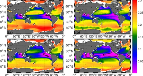
The black contours in Fig. 5 indicate the lateral extent of OMZs for a depth of 300 m (see Fig. S3 for a depth of 900 m). In year 1775, the suboxic volume, defined here as waters with oxygen concentrations of less than 5 mmol m⁻³, equals 3.9×10⁶km³ in both simulations (see Fig. 2d).

An observational estimate of today’s suboxic water volume equals 102×10⁶±15×10⁶km³ for oxygen concentrations less than 20 mmol m⁻³ (Paulmier and Ruiz-Pino, 2009), which is considerably larger than the volume of O₂ concentrations less than 20 mmol m⁻³ in our WB simula-

(7)

Figure 4.Difference (year 3005 minus year 1775) in(a)burial and(b)benthic release flux in mmol P m⁻²a⁻¹for simulation WB.

Figure 5.Oxygen concentration in mol O₂m⁻³at 300 m depth simulated by the(a)control simulation in year 1775 (representative for both REF and WB model runs in year 1775),(b)the World Ocean Atlas in 2009,(c)the control simulation in year 3005 and(d)simulation WB in year 3005. The black contour lines at 0.005 mol m⁻³highlight the oxygen minimum zones (OMZs).

tion (WB₂₀₀₅=15.8×10⁶km³). However, in consideration of the studies of Bianchi et al. (2012) and their calculated OMZ volume of 2.28–2.78×10⁶km³, as well as the World Ocean Atlas (WOA₂₀₀₅=4.12×10⁵km³), it can be con- cluded that estimations of the volume of OMZs vary over a wide range and that our results are within this range. Compar- ing our results with observational data from the WOA, a generally good agreement can be found with regard to the spatial distribution of low-oxygen waters (see Fig. 5). The suboxic areas are located in the upwelling regions of the tropical eastern Pacific and eastern Atlantic as well as in the Indian Ocean (see Fig. 5; representative for both simulations in 1775).

During our transient simulations, we find a considerable expansion of OMZs until year 3005 in both simulations (see Figs. 2d and 5). The expansion of the suboxic volume between 300 and 900 m is particularly pronounced in the WB simulation where the OMZs account for 4.85×10⁷km³ in year 3005, i.e. an increase by a factor of 12.4. The control simulation (REF) shows a much smaller increase in the volume of OMZs (1.12×10⁷km³between 300 and 900 m depth). As both simulations display similar climates (see

Fig. 2a), the difference in the oxygen fields is largely due to the differences in the simulated P cycle.

The sea-floor area in contact with suboxic bottom waters, which directly impacts the redox-sensitive benthic burial and P release, shows an increase by more than a factor of 19 (WB1775=3.59×10⁵km²; WB3005=6.95×10⁶km²) in the WB simulation (see Fig. 2d) compared to a factor of 4 increase in the REF simulation (REF1775=2.79×10⁵km²; REF3005=1.2×10⁶km²).

Our present-day results (WB₂₀₀₅=3.8×10⁵km²) compare well with data of the WOA (WOA₂₀₀₅=2.48×10⁵km²).

Somewhat unexpectedly, in our study, an increase in continental weathering does not result in an anoxic ocean under current topography and seawater chemistry – at least not until year 10 000. At the pre-industrial state (year 1775), 0.12 % of all coastal margins are characterised by oxygen concentrations below 0.005 mol m⁻³. While this portion increases by about a factor of 50 to 5.57 % by year 3005, this is too low for the generation of widespread coastal anoxia. Conversely, the global mean oxygen concentration starts to increase again in year 3415 when it has reached a minimum of about two-

(8)

thirds of the pre-industrial oxygen inventory in the WB simulation (see Fig. S1). This suggests that the positive feedback between the release of benthic P and marine net primary production is – in this study, for present-day bathymetry and ge- ography – not the decisive factor for a rapid transition into an anoxic ocean.

4 Uncertainties

Although the model’s subcomponents for weathering, burial and benthic release rates are highly simplified in this study, the simulated global P fluxes fall within the range suggested by earlier studies and observational estimates (Palastanga et al., 2011; Filippelli, 2002; Baturin, 2007; Wallmann, 2010).

The weathering fluxes are calibrated against global mean burial rates under an implicit steady-state assumption, although it is unclear whether the pre-industrial P cycle in the ocean was in equilibrium (Wallmann, 2010). The relatively high P weathering fluxes as well as the assumed indefinite P reservoir in the shelf sediments in our simulations might lead to an overestimation of the effects on the P cycle and OMZs.

In our model, the increase in the P inventory results in a strong increase in ONPP. Contrary to other studies, e.g.

Gregg et al. (2005) or Boyce et al. (2010), in our study the temperature effect overcompensates the stratification effect as described by Sarmiento et al. (2004), Taucher and Os- chlies (2011) and Kvale et al. (2015), and thus leads to an increase in ONPP also in the reference run. While the net effect of warming on ONPP is not well constrained and differs considerably among models, the impact of changing envi- ronmental conditions on export production appears to be better constrained (Taucher and Oschlies, 2011). In agreement with simulations by other models, experiment REF shows a stratification-induced decline in export production, while the increase in P induces an increase in export production in WB. Although we use a coarse-resolution model, the applied sub-grid-scale bathymetry allows the calculation of more ac- curate benthic burial and release fluxes than otherwise possible with such a model. It should also be noted that the benthic release feedback on OMZs might have been more efficient under Cretaceous boundary conditions because the shelf area was considerably larger due to higher sea levels (late Cretaceous shelf area: 46×10⁶km²; present-day shelf area: 26×10⁶km²; Bjerrum et al., 2006). Cretaceous topography might therefore have induced a stronger benthic release feedback, as shown in Tsandev and Slomp (2009).

Filippelli (2002) showed in his study that due to the anthropogenic activities the global, total present-day river input of P has doubled in the last 150 years. In our study, the direct anthropogenic influence, such as agricultural input of P into the system, is excluded and should be considered in future studies even though the human impact is projected to decrease until year 3500 (Filippelli, 2008). Filippelli (2008) and Harrison et al. (2005) estimated a rate of 0.03 Tmol P a⁻¹

and 0.7 Tg P a⁻¹(0.023 Tmol P a⁻¹), respectively, for anthropogenic P delivered to the ocean as a result of fertilisation, deforestation and soil loss as well as sewage in year 3000.

In comparison to our simulated maximum weathering value of 1.09 Tmol P a⁻¹until year 3005, the direct anthropogenic impact seems to be small.

5 Conclusions

This study constitutes a first approach to estimate the potential impact of changes in the marine P cycle on the expansion of global ocean OMZs under global warming on millennial timescales. Model simulations show that the warming- induced increase in terrestrial weathering (see Fig. 3b) leads to an increase in marine P inventory (see Fig. 2b) resulting in an intensification of the biological pump, corroborating the findings by Tsandev and Slomp (2009). As a consequence, oxygen consumption as well as the volume of OMZs increase in our simulations by a factor of 12 over the next millennium (see Figs. 2d and 5).

The positive feedback involving redox-sensitive benthic P fluxes – where the expansion of OMZs leads to an increase in benthic release of P (see Figs. 2c and S1), which in turn enhances biological production and subsequent oxygen consumption (Wallmann, 2010) – has only limited relevance for the expansion of OMZs in this study. Instead, a negative feedback dominates, which involves enhanced weathering and P supply to the ocean, an intensification of the biological carbon pump and associated marine uptake of atmospheric CO2. The atmospheric CO2impacts the surface air temperature through a negative feedback loop, which limits the warming and weathering and, eventually, the expansion of the OMZs. We can therefore conclude that, based on the pa- rameterisations used in this study, the P weathering and biological pump feedback outcompetes the redox-sensitive benthic P-release feedback on millennial timescales. Although the ocean does not become anoxic in our simulations, the benthic P-release feedback may have played a role in past oceanic anoxic events. An increase in shelf areas due to higher sea levels, such as during the Cretaceous, would have led to a more powerful benthic P-release feedback as a much larger sediment area could have been in contact with low- oxygen bottom waters. Whether this different bathymetry alone could result in a more dominant benthic P-release feedback needs to be investigated in future studies.

Code availability. The model data and model code are available at http://data.geomar.de/thredds/catalog/open_access/niemeyer-et-al_

2016/catalog.html.

The Supplement related to this article is available online at doi:10.5194/esd-8-357-2017-supplement.

(9)

Competing interests. The authors declare that they have no con- flict of interest.

Acknowledgements. This work is a contribution to the Son- derforschungsbereich (SFB) 754 “Climate-Biogeochemical Interactions in the Tropical Ocean” and the BMBF project PalMod.

We thank M. Eby for his excellent help with the UVic ESCM and K. F. Kvale and J. Getzlaff for proofreading. Katrin J. Meissner is thankful for UNSW Science Silver- and Goldstar Awards.

The article processing charges for this open-access publication were covered by a Research

Centre of the Helmholtz Association.

Edited by: A. Levermann

Reviewed by: two anonymous referees

References

Archer, D.: A data-driven model of the global cal- cite lysocline, Global Biogeochem. Cy., 10, 511–526, doi:10.1029/96GB01521, 1996.

Baturin, G. N.: Issue of the Relationship between Primary Produc- tivity of Organic Carbon in Ocean and Phosphate Accumula- tion (Holocene-Late Jurassic), Lith. Mineral Res., 42, 318–348, doi:10.1134/S0024490207040025, 2007.

Berner, R. A.: Weathering, plants and the long-term carbon cycle, Geochim. Cosmochim. Ac., 56, 3225–3231, 1991.

Berner, R. A. and Rao, J.-L.: Phosphorus in sediments of the Ama- zon River and estuary: Implications for the global flux of phosphorus to the sea, Geochim. Cosmochim. Ac., 58, 2333–2339, 1994.

Bianchi, D., Dunne, J. P., Sarmiento, J. L., and Galbraith, E. D.: Data-based estimates of suboxia, denitrification, and N₂O production in the ocean and their sensitivities to dissolved O₂, Global Biogeochem. Cy., 26, GB2009, doi:10.1029/2011GB004209, 2012.

Bjerrum, C. J., Bendtsen, J., and Legarth, J. I. F.: Modelling organic carbon burial during sea level rise with reference to the Cretaceous, Geochem. Geophy. Geosy., 7, Q05008, doi:10.1029/2005GC001032, 2006.

Bopp, L., Le Quere, C., Heimann, M., and Manning, A.: Climate- induced oceanic oxygen fluxes: Implications for the contem- porary carbon budget, Global Biogeochem. Cy., 16, 6-1–6-13, doi:10.1029/2001GB001445, 2002.

Bopp, L., Resplandy, L., Orr, J. C., Doney, S. C., Dunne, J. P., Gehlen, M., Halloran, P., Heinze, C., Ilyina, T., Séférian, R., Tjiputra, J., and Vichi, M.: Multiple stressors of ocean ecosystems in the 21st century: projections with CMIP5 models, Biogeosciences, 10, 6225–6245, doi:10.5194/bg-10-6225-2013, 2013.

Boyce, D. G., Lewis, M. R., and Worm, B.: Global phytoplankton decline over the past century, Nature, 466, 591–596, 2010.

Cabré, A., Marinov, I., Bernardello, R., and Bianchi, D.: Oxy- gen minimum zones in the tropical Pacific across CMIP5 models: mean state differences and climate change trends, Biogeo- sciences, 12, 5429–5454, doi:10.5194/bg-12-5429-2015, 2015.

Colmann, A. S. and Holland, H. D.: The global diagenetic flux of phosphorus from marine sediments to the oceans: Redox sensitivity and the control of atmospheric oxygen levels, Marine Au- thigenesis: From Global to Microbial, Spec. Publ. SEPM Soc.

Sediment. Geol., 66, 21–33, 2000.

Compton, J., Mallinson, D., Glenn, C. R., Filippelli, G., Föllmi, K., Shields, G., and Zanin, Y.: Variations in the global phosphorus cycle, Marine Authigenesis: From Global to Microbial, edited by: Glenn, C. R., Prévôt, L., and Lucas, J., SEPM Spec. Publ., 66, 53–75, 2000.

Eby, M., Zickfeld, K., Montenegro, A., Archer, D., Meissner, K. J., Weaver, A. J.: Lifetime of Anthropogenic Climate Change: Millennial Time Scales of Potential CO₂ and Sur- face Temperature Perturbations, J. Climate, 22, 2501–2511, doi:10.1175/2008JCLI2554.1, 2009.

Fanning, A. G. and Weaver, A. J.: An atmospheric energy-moisture model: Climatology, interpentadal climate change and coupling to an ocean general circulation model, J. Geophys. Res., 101, 15111–15128, doi:10.1029/96JD01017, 1996.

Filippelli, G. M.: The Global Phosphorus Cycle, Rev. Mineral.

Geochem., 48, 391–425, doi:10.2138/rmg.2002.48.1, 2002.

Filippelli, G. M.: The Global Phosphorus Cycle: Past, Present, and Future, Elements, 4, 89–95, doi:10.2113/GSELEMENTS.4.2.89, 2008.

Floegel, S., Wallmann, K., Poulson, C. J., Zhou, J., Oschlies, A., Voigt, S., and Kuhnt, W.: Simulating the biogeochemical effects of volcanic CO₂degassing on the oxygen-state of the deep ocean during the Cenomanian/Turonian Anoxic Event (OAE2), Earth.

Planet. Sc. Lett., 305, 371–384, doi:10.1016/j.epsl.2011.03.018, 2011.

Föllmi, K. B.: The phosphorus cycle, phosphogenesis and marine phosphate-rich deposits, Earth-Sci. Rev., 40, 55–124, doi:10.1016/0012-8252(95)00049-6, 1996.

Froelich P. N.: Interactions of the marine phosphorus and carbon cycles, in: The Interaction of Global Biogeochemical Cycles, edited by: Moore, B. and Dastoor, M. N., California Institute of Tech- nology, Pasadena, NASA – JPL Publication 84–21, 141–176, 1984.

Froelich, P. N., Bender, M. L., and Luedtke, N. A.: The marine phosphorus cycle, Am. J. Sci., 282, 474–511, doi:10.2475/ajs.282.4.474, 1982.

Gregg, W. G., Casey, N. W., and McClain, C. R.: Recent trends in global ocean chlorophyll, Geophys. Res. Lett., 32, L03606, doi:10.1029/2004GL021808, 2005.

Handoh, I. and Lenton, T. M.: Periodic mid-Cretaceous oceanic anoxic events linked by oscillations of the phosphorus and oxygen biogeochemical cycles, Global Biogeochem. Cy., 17, 1092, doi:10.1029/2003GB002039, 2003.

Harrison, J., Seitzinger, S. P., Bouwman, F., Caraco, N. F., Beusen, A. H. W., and Vörösmarty, C. J.: Dissolved inorganic phosphorus export to the coastal zone: Results from a spatially ex- plicit, global model, Global Biogeochem. Cy., 19, GB4S03, doi:10.1029/2004GB002357, 2005.

Hibler, W. D.: A dynamic thermodynamic sea ice model, J. Phys.

Oceanogr., 9, 815–846, 1979.

Hofmann, M. and Schellnhuber, H. J.: Ocean acidification: a millennial challenge, Energy Environ. Sci., 3, 1883–1896, doi:10.1039/C000820F, 2010.

(10)

Hunke, E. C. and Dukowicz, J. K.: An Elastic-Viscous-Plastic Model for Sea Ice Dynamics, J. Phys. Oceanogr., 27, 1849–1867, 1997.

Ingall, E. and Jahnke, R.: Evidence for enhanced phosphorus regeneration from marine sediments overlain by oxygen depleted waters, Geochim. Cosmochim. Ac., 58, 2571–2575, doi:10.1016/0016-7037(94)90033-7, 1994.

Keller, D. P., Oschlies, A., and Eby, M.: A new marine ecosystem model for the University of Victoria Earth System Climate Model, Geosci. Model Dev., 5, 1195–1220, doi:10.5194/gmd-5- 1195-2012, 2012.

Kraal, P., Slomp, C. P., Reed, D. C., Reichart, G.-J., and Poulton, S. W.: Sedimentary phosphorus and iron cycling in and below the oxygen minimum zone of the northern Arabian Sea, Biogeo- sciences, 9, 2603–2624, doi:10.5194/bg-9-2603-2012, 2012.

Kvale, K. F., Meissner, K. J., and Keller, D. P.: Potential increasing dominance of heterotrophy in the global ocean, Environ. Res.

Lett., 10, 074009, doi:10.1088/1748-9326/10/7/074009, 2015.

Lenton, T. M. and Britton, C.: Enhanced carbonate and silicate weathering accelerates recovery from fossil fuel CO₂ perturbations, Global Biogeochem. Cy., 20, B3009, doi:10.1029/2005GB002678, 2006.

Lenton, T. M. and Watson, A. J.: Redfield revisited. 1. Regulation of nitrate, phosphate, and oxygen in the ocean, Global Biogeochem.

Cy., 14, 225–248, doi:10.1029/1999GB900065, 2000.

Manabe, S. and Stouffer, R. J.: Multiple-Century Response of a Coupled Ocean-Atmosphere Model to an increase of Atmo- spheric Carbon Dioxide, J. Climate, 7, 5–23, 1993.

Meinshausen, M., Smith, S. J., Calvin, K., Daniel, J. S., Kainuma, M. L. T., Lamarque, J.-F., Matsumoto, K., Montzka, S. A., Raper, S. C. B., Riahi, K., Thomson, A., Velders, G. J. M., and van Vu- uren, D. P. P.: The RCP greenhouse gas concentrations and their extensions from 1765 to 2300, Climatic Change, 109, 213–241, doi:10.1007/s10584-011-0156-z, 2011.

Meissner, K. J., Weaver, A. J., Matthews, H. D., and Cox, P. M.:

The role of land surface dynamics in glacial inception: a study with the UVic Earth System Model, Clim. Dynam., 21, 515–537, doi:10.1007/s00382-003-0352-2, 2003.

Meissner, K. J., McNeil, B., Eby, M., and Wiebe, E. C.: The im- portance of the terrestrial weathering feedback for multimil- lenial coral reef habitat recovery, Global Biogeochem. Cy., 26, GB3017, doi:10.1029/2011GB004098, 2012.

Monteiro, F. M., Pancost, R. D., Ridgwell, A., and Donnadieu, Y.: Nutrients as the dominant control on the spread of anoxia and euxinia across the Cenomanian-Turonian oceanic anoxic event (OAE2): Model-data comparison, Paleoceanography, 27, PA4209, doi:10.1029/2012PA002351, 2012.

Moore, J. K., Lindsay, K., Doney, S. C., Long, M. C., and Misumi, K.: Marine Ecosystem Dynamics and Biogeochemical Cycling in the Community Earth System Model [CESM1(BGC)]: Compar- ison of the 1990s with the 2090s under the RCP4.5 and RCP8.5 Scenarios, J. Climate, 26, 9291–9312, doi:10.1175/JCLI-D-12- 00566.1, 2013.

Oschlies, A., Schulz, K. G., Riebesell, U., and Schmittner, A.:

Simulated 21^st century’s increase in oceanic suboxia by CO₂- enhanced biological carbon export, Global Biogeochem. Cy., 22, GB4008, doi:10.1029/2007GB003147, 2008.

Pacanowski, R. C.: MOM 2 Documentation User’s Guide and Ref- erence Manual, Version 1.0. GFDL Technical Report, 1995.

Palastanga, V., Slomp, C. P., and Heinze, C.: Long-term con- trols on ocean phosphorus and oxygen in a global biogeochemical model, Global Biogeochem. Cy., 25, GB3024, doi:10.1029/2010GB003827, 2011.

Paulmier, A. and Ruiz-Pino, D.: Oxygen minimum zones (OMZs) in the modern ocean, Prog. Oceanogr., 80, 113–128, doi:10.1016/j.pocean.2008.08.001, 2009.

Payton, A. and McLoughlin, K.: The Oceanic Phosphorus Cycle, Chem. Rev., 107, 563–576, doi:10.1021/cr0503613, 2007.

Redfield, A. C., Ketchum, B. H., and Richards, F. A.: The influence of organisms on the composition of seawater, The Sea, edited by:

Hill, M. N., 2, 26–77, 1963.

Riahi, K., Rao, S., Krey, V., Cho, C., Chirkov, V., Fischer, G., Kin- dermann, G., Nakicenovic, N., and Rafaj, P.: RCP 8.5 – A scenario of comparatively high greenhouse gas emissions, Climatic Change, 109, 33–57, doi:10.1007/s10584-011-0149-y, 2011.

Ruttenberg, K. C.: The global phosphorus cycle. The Global Phos- phorus Cycle. Treatise on Geochemistry, edited by: Schlesinger, W., 585–643, Elsevier, Amsterdam, 2004.

Ruvalcaba Baroni, I., Topper, R. P. M., van Helmond, N. A. G. M., Brinkhuis, H., and Slomp, C. P.: Biogeochemistry of the North Atlantic during oceanic anoxic event 2: role of changes in ocean circulation and phosphorus input, Biogeosciences, 11, 977–993, doi:10.5194/bg-11-977-2014, 2014.

Sabine, C. L., Feely, R. A., Gruber, N., Key, R. M., Lee, K., Bullis- ter, J. L., Wanninkhof, R., Wong, C. S., Wallace, D. W. R., Tilbrook, B., Millero, F. J., Peng, T.-H., Kozyr, A., Ono, T., and Rios, A. F.: The Oceanic Sink for Anthropogenic CO₂, Science, 305, 367–371, doi:10.1126/science.1097403, 2004.

Sarmiento, J. L. and Orr, J. C.: Three-dimensional simulations of the impact of Southern Ocean nutrient depletion on atmospheric CO₂and ocean chemistry, Limnol. Oceanogr., 36, 1928–1950, 1991.

Sarmiento, J. L., Hughes, T. M. C., Stouffer, R. J., and Man- abe, S.: Simulated response of the ocean carbon cycle to anthropogenic climate warming, Letters to Nature, 393, 245–249, doi:10.1038/30455, 1998.

Sarmiento, J. L., Slater, R., Barber, R., Bopp, L., Doney, S. C., Hirst, A. C., Kleypas, J., Mataer, R., Mikolajewicz, U., Monfray, P., Soldatov, V., Spall, S. A., and Stouffer, R.: Response of ocean ecosystems to climate warming, Global Biogeochem. Cy., 18, GB3003, doi:10.1029/2003GB002134, 2004.

Schlanger, S. O. and Jenkyns, H. C.: Cretaceous oceanic anoxic events: causes and consequences, Geologie Mijnbouw, 55, 179–

184, 1976.

Schmidtko, S., Stramma, L., and Visbeck, M.: Decline in global oceanic oxygen content during the past five decades, Nature, 542, 335–339, doi:10.1038/nature21399, 2017.

Schmittner, A., Oschlies, A., Matthews, H. D., and Galbraith, E.

D.: Future changes in climate, ocean circulation, ecosystems, and biogeochemical cycling simulated for a business-as-usual CO₂ emission scenario until year 4000 AD, Global Biogeochem. Cy., 22, GB1013, doi:10.1029/2007GB002953, 2008.

Semtner, A. J.: A Model for the Thermodynamic Growth of Sea Ice in Numerical Investigations of Climate, J. Phys. Oceanogr., 6, 379–389, 1976.

Slomp, C. P.: Phosphorus cycling in the estuarine and coastal zones:

Sources, sinks, and transformations. Treatise on Estuarine and

(11)

Coastal Science, edited by: Wolanski, E. and McLusky, D., 201–

230, 2011.

Slomp, C. P. and Van Cappellen, P.: The global marine phosphorus cycle: sensitivity to oceanic circulation, Biogeosciences, 4, 155–

171, doi:10.5194/bg-4-155-2007, 2007.

Somes, C. J., Oschlies, A., and Schmittner, A.: Isotopic constraints on the pre-industrial oceanic nitrogen budget, Biogeosciences, 10, 5889–5910, doi:10.5194/bg-10-5889-2013, 2013.

Steinacher, M., Joos, F., Frölicher, T. L., Bopp, L., Cadule, P., Cocco, V., Doney, S. C., Gehlen, M., Lindsay, K., Moore, J. K., Schneider, B., and Segschneider, J.: Projected 21st century decrease in marine productivity: a multi-model analysis, Biogeo- sciences, 7, 979–1005, doi:10.5194/bg-7-979-2010, 2010.

Stramma, L., Johnson, G. C., Sprintall, J., and Mohrholz, V.: Ex- panding Oxygen-Minimum Zones in the Tropical Ocean, Sci- ence, 320, 655–658, doi:10.1126/science.1153847, 2008.

Stramma, L., Oschlies, A., and Schmidtko, S.: Mismatch between observed and modeled trends in dissolved upper-ocean oxygen over the last 50 yr, Biogeosciences, 9, 4045–4057, doi:10.5194/bg-9-4045-2012, 2012.

Taucher, J. and Oschlies, A.: Can we predict the direction of marine primary production change under global warming?, Geo- phys. Res. Lett, 38, L02603, doi:10.1029/2010GL045934, 2011.

Tsandev, I. V. and Slomp, C. P.: Modelling phosphorus cycling and carbon burial during Cretaceous Oceanic Anoxic Events, Earth Planet. Sc. Lett., 286, 71–79, doi:10.1016/j.epsl.2009.06.016, 2009.

Tyrell, T.: The relative influences of nitrogen and phosphorus on oceanic primary production, Nature, 400, 525–531, doi:10.1038/22941, 1999.

Wallmann, K.: Phosphorus imbalance in the global ocean?, Global Biogeochem. Cy., 24, GB4030, doi:10.1029/2009GB003643, 2010.

Weaver, A. J., Eby, M., Wiebe, E. C., Bitz, C. M., Duffy, P. B., Ewen, T. L., Fanning, A. F., Holland, M. M., MacFadyen, A., Matthews, H. D., Meissner, K. J., Saenko, O., Schmittner, A., Wang, H., and Yoshimori, M.: The UVic Earth System Cli- mate Model: Model Description, Climatology and Applications to Past, Present and Future Climates, Atmos. Ocean, 39, 361–

428, doi:10.1080/07055900.2001.9649686, 2001.

Yool, A., Popova, E. E., Coward, A. C., Bernie, D., and Anderson, T. R.: Climate change and ocean acidification impacts on lower trophic levels and the export of organic carbon to the deep ocean, Biogeosciences, 10, 5831–5854, doi:10.5194/bg-10-5831-2013, 2013.