Calibration of a simple and a complex model of global marine biogeochemistry

https://doi.org/10.5194/bg-14-4965-2017

© Author(s) 2017. This work is distributed under the Creative Commons Attribution 3.0 License.

Calibration of a simple and a complex model of global marine biogeochemistry

Iris Kriest

GEOMAR Helmholtz-Zentrum für Ozeanforschung Kiel, Düsternbrooker Weg 20, 24105 Kiel, Germany Correspondence to:Iris Kriest (ikriest@geomar.de)

Received: 1 March 2017 – Discussion started: 6 March 2017

Revised: 19 August 2017 – Accepted: 1 September 2017 – Published: 8 November 2017

Abstract. The assessment of the ocean biota’s role in cli- mate change is often carried out with global biogeochemi- cal ocean models that contain many components and involve a high level of parametric uncertainty. Because many data that relate to tracers included in a model are only sparsely observed, assessment of model skill is often restricted to trac- ers that can be easily measured and assembled. Examination of the models’ fit to climatologies of inorganic tracers, after the models have been spun up to steady state, is a common but computationally expensive procedure to assess model performance and reliability. Using new tools that have be- come available for global model assessment and calibration in steady state, this paper examines two different model types – a complex seven-component model (MOPS) and a very simple four-component model (RetroMOPS) – for their fit to dissolved quantities. Before comparing the models, a sub- set of their biogeochemical parameters has been optimised against annual-mean nutrients and oxygen. Both model types fit the observations almost equally well. The simple model contains only two nutrients: oxygen and dissolved organic phosphorus (DOP). Its misfit and large-scale tracer distribu- tions are sensitive to the parameterisation of DOP produc- tion and decay. The spatio-temporal decoupling of nitrogen and oxygen, and processes involved in their uptake and re- lease, renders oxygen and nitrate valuable tracers for model calibration. In addition, the non-conservative nature of these tracers (with respect to their upper boundary condition) in- troduces the global bias (fixed nitrogen and oxygen inven- tory) as a useful additional constraint on model parameters.

Dissolved organic phosphorus at the surface behaves antago- nistically to phosphate, and suggests that observations of this tracer – although difficult to measure – may be an important asset for model calibration.

1 Introduction

Global biogeochemical ocean models are now routinely used to assess the ocean biota’s role in climate change. Although these models have become ever more complex with respect to the number of biogeochemical tracers they contain, they are often calibrated only against a subset of their components, mostly nutrients, oxygen and components of the carbon cycle (e.g. Bacastow and Maier-Reimer, 1991; Ilyina et al., 2013;

Cocco et al., 2013; Cabre et al., 2015).

There has been an intensive discussion about the neces- sary level of marine ecosystem model complexity, mostly on a theoretical basis, or in a local or regional context (e.g.

Anderson, 2005, 2006; Le Quere, 2006; Flynn, 2006; Leles et al., 2016; Shimoda and Arhonditsis, 2016). It remains an open question as to whether additional complexity is of ad- vantage for representing biogeochemical processes and trac- ers on a global scale (i.e. for processes acting on rather long timescales and large space scales). For example, Kriest et al.

(2010, 2012) found no large differences when comparing model skill with respect to oxygen and phosphate across a range of models of different complexity, but quite large ef- fects of parameter settings when applying a coarse examina- tion of the parameter space.

However, a thorough and dense scan of the parameter space would be required for a fair assessment of the virtues of models of different complexity. Such a scan usually requires many model evaluations, which, given the long equilibration timescales of coupled global models (Khatiwala, 2008; Wun- sch and Heimbach, 2008; Primeau and Deleersnijder, 2009;

Siberlin and Wunsch, 2011), is difficult to carry out. For as- sessment of only surface properties and processes, a short model spin-up may be sufficient; however, on a global scale, many centuries to millennia of coupled model simulations

are necessary in order to remove the drift in biogeochemical tracer fields and fit to observed properties (Kriest and Os- chlies, 2015; Séférian et al., 2016).

Only recently tools have become available that allow for a reduction in simulation times, such as the Transport Matrix Method (TMM, Khatiwala et al., 2005), which replaces the ocean circulation model with an efficient “offline” circula- tion, or methods that solve for steady-state tracer fields using Newton’s method. The latter require either the inversion of the Jacobian (e.g. Kwon and Primeau, 2006), or the appli- cation of matrix-free Newton–Krylov (MFNK, Khatiwala, 2008; Li and Primeau, 2008) to compute the steady-state solution. Surrogate-based optimisation replaces the original and computationally expensive model by a so-called surro- gate, which is created from a less accurate but computation- ally cheaper model. The latter is corrected to reduce the mis- alignment between the two solutions. Priess et al. (2013) ap- plied this method, together with the TMM, to recover param- eters of a simple global biogeochemical model; the surrogate in their case consisted of shorter (decades) spin-ups.

The gain in computational efficiency resulting from these methods can then be used for a systematic calibration of global biogeochemical models. For example, Kwon and Primeau (2006, 2008) used global climatological data sets of phosphate, inorganic carbon and alkalinity to calibrate a sim- ple global biogeochemical model. The misfit between ob- served and simulated phosphate was used by DeVries et al.

(2014) to calibrate parameters related to particle properties in a simple two-component, nutrient-restoring model. In a sim- ilar approach Holzer et al. (2014) optimised parameters for opal production and dissolution against observed silicate.

Letscher et al. (2015) switched between a complex and a sim- ple model of ocean biogeochemistry to estimate production and decay rates of dissolved organic phosphorus on a global scale.

All these biogeochemical models employed in global pa- rameter estimates were of a low level of biogeochemical complexity. One reason for this restriction might be asso- ciated with the variety of timescales associated with more complex models. Piwonski and Slawig (2016) used MFNK to evaluate the steady state of simple and complex biogeochem- ical models. They noted that “[. . . ] for more complex mod- els the Newton method requires more attention to solver pa- rameter settings [. . . ]” (Piwonski and Slawig, 2016), which may be related to the highly nonlinear structure of these models. The nonlinearity, and the large number of parame- ters, also complicates their simultaneous optimisation (Ward et al., 2010). On a global scale, these problems are ampli- fied by the sparsity of observations of organism groups, par- ticularly of higher trophic levels. Observations of dissolved inorganic constituents, on the other hand, are much more fre- quent and therefore provide more information on the spatio- temporal variability of these tracers.

Recently, Kriest et al. (2017) combined the TMM with an estimation of a distribution algorithm (covariance ma-

trix adaption evolution strategy, CMA-ES), to optimise six biogeochemical parameters of a seven-component model against global climatologies of annual mean phosphate, ni- trate and oxygen. They showed that annual mean tracer con- centrations did not provide much information on parame- ters related to the dynamic biological processes taking place in the euphotic zone, but that parameters related to long timescales and large space scales (e.g. the remineralisation length scale or so-called “Martinb”; see also Kriest et al., 2012) could be estimated from these observations. The large uncertainty associated with surface parameter estimates can be attributed to the relatively small volume of the surface ocean, leading to a misfit that is dominated by deep-ocean observations.

Replacing the misfit function by a metric that targets the surface ocean, and/or contains additional observations that provide information on plankton, could be one way to re- solve this indeterminacy. Alternatively, one could omit these parameters from the optimisation and focus on parameters more tightly connected to the meso- and bathypelagic ocean.

A more drastic measure lies in downscaling the biogeochem- ical model to a simpler system, that only contains compo- nents with a counterpart in global, quasi-synoptic data sets.

The latter procedure may help to elucidate which level of complexity is required to represent and investigate global dis- tribution and patterns of biogeochemical tracers.

This paper examines the latter two potential solu- tions: firstly, I investigate if parameters related to oxidant- dependent decay in the mesopelagic zone are better con- strained by this type of misfit function. This is done by re- placing four parameters of the optimisation carried out by Kriest et al. (2017) by parameters related to oxidant affin- ity of remineralisation, and – to account for the possible al- terations in fixed nitrogen turnover – by the maximum ni- trogen fixation rate. Secondly, given the successful param- eter optimisation of simpler models noted above, and also to acknowledge the fact that these models have been pop- ular and quite successful in global simulations of ocean biogeochemistry (e.g. Bacastow and Maier-Reimer, 1990, 1991; Matear and Hirst, 2003; Kwon and Primeau, 2006;

Dutkiewicz et al., 2006), this paper presents an optimised model, which has been derived from downscaling the seven- component model MOPS (Kriest and Oschlies, 2015; Kriest et al., 2017) to a model that retains only three abiotic dis- solved tracers (phosphate, nitrate and oxygen) and one bi- otic tracer (dissolved organic phosphorus, DOP). This new model, which I refer to as “RetroMOPS”, includes the oxi- dant dependency of MOPS, but is otherwise very similar to models applied earlier in global models. In contrast to some of these models (Marchal et al., 1998; Najjar et al., 2007) it assumes no relaxation to observed tracer fields, but simulates fully prognostic changes in surface production, as in Bacas- tow and Maier-Reimer (1991), Maier-Reimer (1993), Matear and Hirst (2003) and Parekh et al. (2005).

After a brief presentation of model MOPS (Kriest and Os- chlies, 2015), the downscaled model RetroMOPS is intro- duced, followed by an outline on circulation, optimisation and experimental design (Sect. 2). In Sect. 3 results from op- timisation of both MOPS and RetroMOPS are presented and discussed. The paper closes with conclusions drawn from these experiments.

2 Models, experiments and optimisations 2.1 The MOPS model

The MOPS model (Kriest and Oschlies, 2015) is based on phosphorus and simulates seven compartments. Phosphate, phytoplankton, zooplankton, DOP and detritus are calcu- lated in units of millimoles of phosphorus per cubic me- tre (mmol P m⁻³). Oxygen is coupled to the P cycle with a constant stoichiometry given by R_−O2:P. Aerobic rem- ineralisation of organic matter follows a saturation curve, with half-saturation constantK_O2. Aerobic remineralisation ceases when oxygen declines; at the same time, denitrifica- tion takes over, as long as nitrate is available above a defined threshold, DIN_min. Like the oxic process, suboxic reminer- alisation follows a saturation curve for oxidant nitrate, with half-saturation constantK_DIN. MOPS does not explicitly re- solve the different oxidation states of inorganic nitrogen (ni- trite, N2O, ammonium), but assumes immediate coupling of the different processes involved in nitrate reduction, the end product being dinitrogen (see also Paulmier et al., 2009; Kri- est and Oschlies, 2015). All organic components are charac- terised by a constant N:P stoichiometry ofd=16. Loss of fixed nitrogen is balanced by a simple parameterisation of nitrogen fixation by cyanobacteria, which relaxes the nitrate- to-phosphate ratio to d with a time constant,µ^∗_NFix. In the long term, nitrogen fixation balances the simulated loss of fixed nitrogen via denitrification, although they may occur in distant areas (see Kriest and Oschlies, 2015, for more de- tails).

Detritus sinks with a vertically increasing sinking speed:

w=a z. Assuming a constant degradation rate r, in equi- librium this would result in a particle flux curve given by F (z)∝z^−b, withb=r/a. For better comparison with values ofbderived from observations (e.g. Martin et al., 1987; Van Mooy et al., 2002; Buesseler et al., 2007), and with the sim- pler model RetroMOPS (see below),ais expressed in terms of b(assuming constant, nominalr=0.05 d⁻¹). A fraction of detritus deposited at the sea floor (at the bottom of the deepest vertical box) is buried instantaneously in some hy- pothetical sediment. The fraction buried depends on the de- position rate onto the sediment. Non-buried detritus is resus- pended into the last box of the water column, where it is treated as regular detritus. The phosphorus budget is closed on an annual timescale through resupply via river runoff.

More details about the biogeochemical model and parame-

ters and their effects on model behaviour can be found in Kriest and Oschlies (2013) and Kriest and Oschlies (2015).

2.2 Model RetroMOPS

MOPS’ structure has been simplified by skipping the ex- plicit simulation of phytoplankton, zooplankton and detritus (see Fig. S1 in the Supplement). The remaining equations of, and functional relationships between, phosphate, nitrate, oxygen and DOP have been parameterised similar to MOPS.

Because the downscaled model resembles so many features of earlier biogeochemical models simulated in a global con- text (e.g. Bacastow and Maier-Reimer, 1991; Maier-Reimer, 1993; Matear and Hirst, 2003), but keeps the oxidant depen- dency of MOPS, the model is named “RetroMOPS”.

2.2.1 Primary production

Like MOPS, RetroMOPS calculates primary production only in the euphotic zone, which, in the current configuration, is confined to the upper two numerical layers (k_EZ=2, z= 0–120 m). As in Kriest et al. (2010, 2012) phytoplankton is parameterised with a constant concentration of PHY= 0.02 mmol P m⁻³, which is the mean phytoplankton concen- tration in the upper 120 m of two optimised model set-ups MOPS^◦Sand MOPS^◦D(see below). Using this constant phy- toplankton concentration, RetroMOPS calculates light- and nutrient-dependent primary productionP in each layerkas follows:

P (k)

= (

µ_PHYPHY min

f (I (k)),_K ^L(k)

PHY+L(k)

:k≤k_EZ

0 :k > k_EZ

, (1)

where f (I (k)) defines light-limitation, µPHY is the temperature-dependent maximum growth rate of phyto- plankton, and L determines the limiting nutrient: L(k)= min(PO4(k),DIN(k)/d)(see Kriest and Oschlies, 2015, for more details). Note that, with the given parameters for nu- trient and light affinity, the resulting specific growth rates (P (k)/PHY) of optimised MOPS and RetroMOPS are quite similar (0.127 d⁻¹ for MOPS and 0.102 d⁻¹ for Retro- MOPS).

2.2.2 The fate of primary production: export, DOP production and remineralisation

Instead of resolving heterotrophic processes (zooplankton grazing, excretion and egestion) at the sea surface explic- itly, in RetroMOPS a fractionσ of organic matter fixed pho- tosynthetically is immediately released as dissolved organic phosphorus. DOP then decays to phosphate and nitrate with a constant rateλ. To allow for a potential fast recycling loop at the surface, RetroMOPS parameterises an additional de- cay rate,λ_s, that affects DOP only in the first two layers. By

doing so, the model mimics multiple DOP fractions with dif- ferent decay rates, as observed by Hopkinson et al. (2002).

The remaining fraction of production, 1−σ, of each layer in the euphotic zone is exported to the layers below, where it immediately remineralises to nutrients, following a power- law of depth. The discretised form for fluxF into boxj from all (surface) source layersk, with 1≤k≤k_EZis then given by the following:

F (j )=

k=kEZ

X

k=1

P (k) (1−σ ) 1z(k) z(j )

z(k+1) −b

forj > k, (2)

where1z(k) denotes the thickness of a numerical (source) layer, andz(j )is the depth of the upper boundary of layerj. The flux divergence,D=dF /dz, for any boxjin discretised form is defined by

D(j )=F (j−1)−F (j )

1z(j ) . (3)

Neglecting oxidant dependency of decay, the entire flux di- vergence D(j )would be released as phosphate and nitrate, with equivalent oxidant consumption. It is, however, possi- ble that oxidants become depleted at some location. Earlier models in this case continued the degradation of organic mat- ter, thereby implicitly assuming unspecified oxidants (e.g.

Marchal et al., 1998; Matear and Hirst, 2003; Najjar et al., 2007; Kriest et al., 2010, 2012). In contrast, RetroMOPS, like MOPS, accounts for suppression of remineralisation (oxic or suboxic) in the absence of sufficient oxidants, by assuming saturation curves for the limitation by either oxygen or ni- trate. The amount of organic matter available for oxidation is given by the decay of dissolved organic matter,λDOP, and by the flux divergence,D(j )(Eq. 3). The discretised flux di- vergence, that can actually be remineralised with available oxidants (oxygen and/or nitrate),D^eff(j ), is then determined by

D^eff(j )=D(j ) s_O2(j )+s_DIN(j )

, (4)

where sO₂(j ) and sDIN(j ) represent the oxidant limitation terms, expressed as saturation curves lO₂ and lNO₃ for ei- ther oxygen (oxic remineralisation) or nitrate (denitrifica- tion), with half-saturation constantsK_O2andK_DIN. Denitrifi- cation is further inhibited by oxygen via(1−l_O2), resulting in s_O2(j )+s_DIN(j )=1 (see also Eqs. 15–27 of Kriest and Os- chlies, 2015). In all models oxic remineralisation only takes place down to a a lower threshold of O₂=4 mmol m⁻³. The lower threshold for denitrification is determined by parame- ter DIN_min, and subject to optimisation.

The flux divergence that cannot be remineralised under the given concentrations of oxidants is added as additional flux divergence to the layer below:

D(j+1)=D(j+1)+

D(j )−D^eff(j ) 1z(j ) 1z(j+1), (5)

where againD^eff(j+1)is evaluated. In the bottom layer the remaining flux that has not been remineralised in the water column eventually enters the sediment.

2.2.3 Benthic exchanges

Models that implicitly assume unspecified oxidants often prescribe a zero boundary flux, i.e. all organic matter in the last bottom box is degraded instantaneously (e.g. Marchal et al., 1998; Matear and Hirst, 2003; Najjar et al., 2007;

Yool et al., 2011). Both MOPS and RetroMOPS have to take

“leftover” organic matter flux into account, that arrives unde- graded at the sea floor because of incomplete remineralisa- tion in the water column. The explicit detritus compartment in MOPS allows for only partial burial at the sea floor, which may result in detritus accumulation in the deepest model box (see Kriest and Oschlies, 2013). Because there is no such detritus compartment in RetroMOPS, all flux arriving at the sea floor is buried immediately. Therefore, MOPS and Retro- MOPS differ with respect to their lower boundary condition.

2.2.4 Nitrogen fixation

Both RetroMOPS and MOPS do not explicitly simulate cyanobacteria, but assume zero net growth of these organ- isms, parameterised as an immediate release of fixed nitrogen as nitrate:

S(k)

=

(µ^∗_NFixf₁(T(k)) f₂(DIN(k),PO₄(k)) :k≤k_EZ

0 :k > k_EZ, (6)

wheref1 parameterises the temperature dependence of ni- trogen fixation with a second-order polynomial approxima- tion of the function by Breitbarth et al. (2007) andf2reg- ulates the relaxation of the nitrate:phosphate ratio towards the global observed stoichiometric ratio ofd=16. The max- imum nitrogen fixationµ^∗_NFix (mmol N m⁻³d⁻¹) parame- terises an implicit cyanobacteria population. As in MOPS, on long timescales nitrogen fixation balances the simulated loss of fixed nitrogen via denitrification, although the regions of nitrogen loss and gain can be spatially segregated (Kriest and Oschlies, 2015).

2.2.5 Source minus sinks

Combining the above-mentioned processes and interactions, the time rate of change in each layerkfor phosphate, nitrate, oxygen and DOP due to biogeochemical processes are

S^PO4= −P

|{z}

production

+ λ_sDOP

| {z }

surface decay

+[D+λDOP]

s_O2+s_DIN

| {z }

decay and flux divergence

(7)

S^DOP=σDOPP

| {z }

release

− λsDOP

| {z }

surface decay

−λDOP

sO₂+sDIN

| {z }

decay

(8)

S^O2=R−O₂:PP

| {z }

production

−R−O₂:PλsDOP

| {z }

surface decay

−R−O₂:P

D+λDOP^∗ sO₂

| {z }

decay and flux divergence

(9)

S^DIN= −d P

| {z }

production

+ S

|{z}

N-fixation

+ d λ_sDOP

| {z }

surface decay

+[D+λDOP]

s_O2d−s_DINR_−NO3:P

| {z }

decay and flux divergence

. (10)

To summarise, RetroMOPS is similar to model “N-DOP” of Kriest et al. (2010, 2012), to the phosphorus component of the model presented by Parekh et al. (2005) or to the mod- els presented by Bacastow and Maier-Reimer (1991) and Maier-Reimer (1993), the exception being details of primary production at the sea surface, and the explicit parameteri- sation of oxidant-dependent remineralisation. By assuming constant cyanobacteria biomass, and a relaxation of the ni- trate:phosphate ratio via immediate release of fixed nitro- gen, its parameterisation of nitrogen fixation is similar to the one described by Maier-Reimer et al. (2005) and Ilyina et al.

(2013). Because RetroMOPS lacks explicit phytoplankton, zooplankton and detritus, it has eight fewer tunable parame- ters than MOPS.

2.3 Circulation and physical transport

All model simulations apply the Transport Matrix Method (Khatiwala, 2007, github.com/samarkhatiwala/tmm) for tracer transport, with monthly mean transport matrices (TMs), wind, temperature and salinity (for air–sea gas ex- change) derived from a 2.8^◦global configuration of the MIT ocean model, with 15 levels in the vertical, as described in Marshall et al. (1997) and Dutkiewicz et al. (2005). The cir- culation model was forced with climatological annual cycles of wind, heat and freshwater fluxes, and subject to a weak restoring of surface temperature and salinity to observa- tions. Its configuration is similar to that applied in the Ocean Carbon-cycle Model Intercomparison Project (OCMIP) (Orr et al., 2000), which has been assessed against observations of temperature, salinity and mixed-layer depth (Doney et al., 2004), CFCs (Dutay et al., 2002; Matsumoto et al., 2004), and radiocarbon (Matsumoto et al., 2004; Graven et al., 2012). Overall, its performance is comparable to other global models.

Using this efficient offline approach, with a time step length of 1/2 day for tracer transport and 1/16 day for bio- geochemical interactions, a simulation of 3000 years requires about 0.5–1.5 h on 4 nodes (24-core Intel Xeon Ivybridge) at a high-performance computing centre (www.hlrn.de). Af- ter 3000 years most tracers have approached steady state (see

also Kriest and Oschlies, 2015, for long time trends of MOPS simulated in a different circulation), and the transient of the misfit function becomes very small (see Fig. S2). The last year is used for model analysis and evaluation of the misfit function.

2.4 Optimisation algorithm

Optimisation of parameters is carried out using an estima- tion of distribution algorithm, namely the covariance ma- trix adaption evolution strategy (Hansen and Ostermeier, 2001; Hansen, 2006). The application of this algorithm to the coupled biogeochemistry–TMM framework has shown good performance with respect to quality and efficiency (in terms of function evaluations) and is described only briefly below.

More details about the algorithm, its set-up and coupling to the global biogeochemical model can be found in Kriest et al.

(2017).

Letnbe the number of biogeochemical parameters to be estimated. In each iteration (“generation”) the algorithm de- fines a population ofλindividuals (biogeochemical parame- ter vectors of lengthn), withλ=10 (derived from the default parameterλ=4+3 ln(n), Hansen and Ostermeier, 2001).

The candidate vectors are sampled from a multi-variate nor- mal distribution, which generalises the usual normal distri- bution, also known as Gaussian distribution, fromRto the vector spaceRⁿ.

Following the simulation of theseλindividual model set- ups to steady state (3000 years), the misfit function is evalu- ated, and information of the current as well as previous gen- erations is used to update the probability distribution inRⁿ such that the likelihood to sample good solutions increases.

Usually, the realisation of the probability distribution update ensures that information of former solutions fades out slowly, resisting for several iterations. Therefore, the population (the number of model simulations per generation) in CMA-ES is smaller, and of less computational demand, than in classical evolutionary algorithms. Nevertheless, CMA-ES can still, to a certain degree, perform well with misfit functions charac- terised by a rough topography (Kriest et al., 2017).

2.5 Misfit function

As in Kriest et al. (2017) the misfit to observationsJ is de- fined as the root mean square error (RMSE) between simu- lated and observed annual mean phosphate, nitrate and oxy- gen concentrations (Garcia et al., 2006a, b), mapped onto the three-dimensional model geometry. Although regridding the observations onto the coarser model geometry removes some of the variability, this method is computationally more effi- cient in an optimisation framework. Also, a sensitivity study with a similar coupled model showed that accounting for the variance inherent in the observational data and arising from regridding did not have a large influence on the misfit (Kriest et al., 2010).

Table 1.Experimental set-up of optimisation. Parameters that stay fixed are highlighted. For parameters subject to optimisation we indicate the assigned a priori lower and upper parameter boundary (parameter range,R^A₂) for optimisation in square brackets; n/a: not applicable for this model.

Experiment MOPS^r MOPS^◦S MOPS^◦D RetroMOPS^r RetroMOPS^◦ Unit

σ n/a n/a n/a 0.67 [0.4–0.8]

λs n/a n/a n/a 0 [0.0–3.6] yr⁻¹

λ 0.17 0.17 0.17 0.36 [0.036–3.6] yr⁻¹

Ic 24 [4–48] 9.65 9.65 9.65 W m⁻²

K_PHY 0.03125 [0.001–0.5] 0.5 0.5 0.5 mmol P m⁻³

µ_ZOO 2 [1–3] 1.89 n/a n/a d⁻¹

κ_ZOO 3.2 [1.6–4.8] 4.55 n/a n/a (d mmol P m⁻³)⁻¹

b^∗ 0.858 [0.4–1.8] [0.4–1.8] 1.0725 [0.4–1.8]

R_−O2:P 170 [150–200] [150–200] 171.7 171.7 mmol O₂: mmol P

µ_NFix 2 2 [1–3] 1.19 1.19 nmol N d⁻¹

DIN_min 4 4 [1–16] 15.80 15.80 mmol N m⁻³

K_O2 2 2 [1–16] 1.0 1.0 mmol O₂m⁻³

KDIN 8 8 [2–32] 31.97 31.97 mmol N m⁻³

∗Note that fromb(the optimised parameter) in MOPS we calculate the rate of vertical increase in sinking speedaofw=a z, viaa=r/b. For rwe assume nominal detrital remineralisation ofr=0.05 d⁻¹. The resulting values foraare 0.058275 (b=0.858), 0.0278 (lower boundary) and 0.125 (upper boundary).

Deviations between model and observations are weighted by the volume of each individual grid box, Vi, expressed as fraction of total ocean volume,VT. The resulting sum of weighted deviations is then normalised by the global mean concentration of the respective observed tracer:

J =

3

X

j=1

J (j )=

3

X

j=1

1 o_j

v u u t

N

X

i=1

(m_i,j−o_i,j)²Vi

VT

, (11)

wherej =1,2,3 indicates the tracer type andi=1, . . ., N are the model locations forN=52 749 model grid boxes;o_j is the global average observed concentration of the respective tracer. The termsm_i,j ando_i,j are model and observations, respectively. By weighting each individual misfit with vol- ume,J serves more as a long-timescale geochemical estima- tor, in contrast to a misfit function that, for example, focuses on (rather fast) turnover in the surface layer, or resolves the seasonal cycle.

2.6 Optimisation of MOPS

Based on a “hand-tuned”, a priori set-up of MOPS (Kri- est and Oschlies, 2015), which hereafter is referred to as MOPS^r, Kriest et al. (2017) presented an optimisation of mostly surface-related parameters (hereafter referred to as MOPS^◦S). They chose a very wide range of parameter types, across all trophic levels and acting on different time and space scales. In that optimisation many of the surface param- eters were difficult to constrain, because of a misfit function that consists mostly of observations in the deep ocean. Op- timisation MOPS^◦Dpresented here applies the same metric,

but focuses on parameters in subsurface waters. The selection of parameters to be optimised is motivated by the large uncer- tainty regarding extent and expansion of oxygen minimum zones in models (Cocco et al., 2013; Cabre et al., 2015), and because little knowledge exists about their values, or even parameterisations.

ParameterK_O2 determines the affinity of the aerobic rem- ineralisation to oxygen, and the gradual transition from this process to denitrification (see Eqs. 15 and 20 of Kriest and Oschlies, 2015).K_DINdetermines the affinity of denitrifica- tion to nitrate. Parameter DIN_min defines the lower thresh- old for the onset of denitrification. MOPS^◦D also optimises the maximum rate of nitrogen fixation, µ^∗_NFix, which bal- ances fixed nitrogen loss through denitrification. The fifth and sixth parameter to be estimated are the oxygen require- ment per mole of phosphorus remineralised, R−O₂:P, and the flux (or remineralisation) length scale, b. Upper and lower boundaries of parameters to be optimised have been set to a rather wide range (Table 1), to allow optimisation to explore a wide range of potential parameters. The op- timal parameters of MOPS^◦S for light and nutrient affin- ity of phytoplankton, zooplankton grazing and its mortality are retained in MOPS^◦D (Table 1). Therefore optimisation MOPS^◦Dbuilds upon a previous tuning of surface processes.

Most of the processes affected by the parameters to be optimised take place in suboxic waters, e.g. of the eastern equatorial Pacific (EEP). Given the coarse model geometry, it is possible that circulation dynamics are not represented well in the model. To investigate the influence of observa- tions within this region on misfit function and parameter es- timates, MOPS^◦D is repeated with a reduced data set, that

excludes the EEP (here: east of 140^◦W, between 10^◦S and 10^◦N) from the misfit function. This optimisation is named MOPS^◦_∗^D.

2.7 Optimisation of RetroMOPS

In the RetroMOPS model, processes such as grazing of phy- toplankton, and its subsequent release of organic or inorganic phosphorus are parameterised via a single component, DOP.

Because DOP production and decay regulate the partitioning between sinking and dissolved organic matter, optimisation RetroMOPS^◦targets these parameters, namely σ,λs andλ.

Whileσ, as the parameter that regulates the export ratio, may be more or less well constrained,λsandλboth include a va- riety of processes, which may act on timescales of days to years. Hopkinson et al. (2002) applied a multi-G model to incubations of DOP sampled in surface waters of the mid- dle Atlantic Bight, and measured decay constants for the very labile fraction (32 % of total DOP) of ≈80 yr⁻¹, with a range of 3–254 yr⁻¹. Half of total DOP was in the labile fraction and characterised by a decay constant of≈7 yr⁻¹, ranging from 0.8 to 43 yr⁻¹. However, these observations may not be directly transferable to globally simulated DOP, because most of the simulated ocean is far off the productive shelf areas; further, DOP in RetroMOPS is assumed to mimic a variety of biogeochemical components and processes. In a three-step optimisation study Letscher et al. (2015), who optimised a global model of semi-labile and refractory DOM against observations estimated rates of 0.016 yr⁻¹for semi- labile DOP at the surface, and 0.22 yr⁻¹for semi-labile DOP in the mesopelagic zone, i.e. much lower than suggested by Hopkinson et al. (2002). Summarising, the potential decay rate of the very labile to semi-labile fraction varies over sev- eral orders of magnitude, fromO(0.01)toO(100)yr⁻¹.

Optimisation of RetroMOPS focuses on the dominant la- bile to semi-labile fraction, but allows for some potential fast turnover rates of DOP at the sea surface (towards the values observed by Hopkinson et al., 2002). To obtain a first im- pression on model sensitivity towards these parameters, a set of nine a priori experiments, that varyλ between 0.18 and 0.72 yr⁻¹andλ_s between 0 and 0.36 yr⁻¹, has been carried out (Table 2), which provides a guidance for upper and lower boundaries for optimisation of RetroMOPS. To nevertheless explore the full range of potential decay rates, the maximum possible rate (λ+λs) for optimisation is set to 7.2 yr⁻¹, to- wards the average decay rate of the labile DOP observed by Hopkinson et al. (2002). Optimised RetroMOPS^◦will be compared to the sensitivity experiment with the lowest misfit (λ_s=0,λ=0.36), which is denoted as RetroMOPS^r.

The explicit representation of detritus in MOPS may result in considerable numerical diffusion (particularly on coarse vertical grids as used here; see also Kriest and Oschlies, 2011) and thus in a different estimate of optimalbthan when applying a direct flux curve, such as in RetroMOPS. There- fore,b is included as the fourth parameter to be optimised.

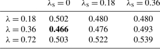
Table 2.Results (misfitJ) of sensitivity experiments with model RetroMOPS, regarding parametersλs andλ for DOP decay rate.

The misfit of the reference scenario RetroMOPS^r is indicated in bold.

λs=0 λs=0.18 λs=0.36 λ=0.18 0.502 0.480 0.480 λ=0.36 0.466 0.476 0.493 λ=0.72 0.503 0.522 0.539

The effect of explicit vs. implicit flux description on param- eter estimate will be discussed in more detail below.

All other parameters (primary production, oxidant- dependent remineralisation, stoichiometry) have been fixed to those obtained in optimisations MOPS^◦S and MOPS^◦D (Table 1). By doing so, optimisation RetroMOPS^◦ builds upon previous optimisations of the more complex MOPS, and overlooks the faint possibility that a parameter that is insensitive in one model, might not be so in another. While it might be desirable to optimise all parameters of RetroMOPS at once, this study rather aims at investigating to what extent a simpler model can serve as a shortcut to the more complex one, given the applied misfit function and observations.

3 Results and discussion

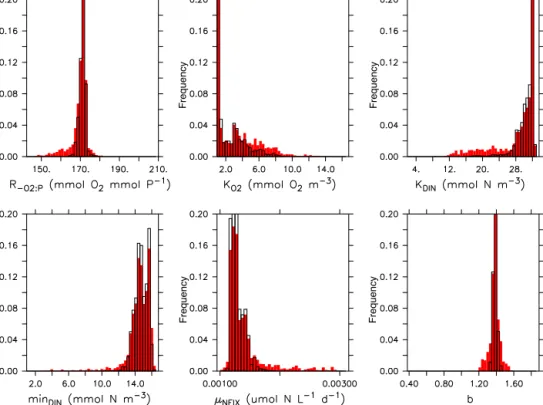
3.1 Optimal remineralisation parameters of MOPS BothR−O₂:Pandbare constrained very well by the observa- tions, as indicated by a well-defined minimum of the misfit function (Fig. S3) and a narrow, almost Gaussian distribution of the best 10–1 % of parameters (Fig. 1). On the other hand, parameters related to the oxidant affinity of remineralisation or nitrogen fixation are determined with lower accuracy. This is also reflected in the rather wide range of candidate solu- tions within 1 ‰ of the best misfit, which vary between 10 and 20 % of their assigned a priori range (Table 3). Thus, in the presence of noise inherent in the observations, some pa- rameters could only be estimated within a quite wide range of uncertainty, a feature that has already been addressed in a one-dimensional model by Löptien and Dietze (2015). So far, the potential consequences of this parametric uncertainty for other metrics (such as extent of oxygen minimum zones, OMZs) and possibly transient scenarios (e.g. their impact on simulated future evolution of OMZ volume) are not known.

The good determination ofbby dissolved inorganic trac- ers is in agreement with earlier studies that applied the same model (Kriest et al., 2017; Schartau et al., 2017). Its optimal value is very close to that obtained in MOPS^◦S, i.e. higher than the value estimated by Kwon and Primeau (2006). Opti- misation of maximum nitrogen fixation rate shows a slightly skewed distribution, but suggests an overall good estimate of this parameter. Optimal parameters for oxidant-dependent

Frequency Frequency

Frequency Frequency

FrequencyFrequency

Figure 1.Parameter distribution of model simulations obtained during the optimisation of MOPS^◦D, whose misfit do not exceed a threshold limit of1J=1.1J^∗(10 %, red bars) or1J=1.01J^∗(1 %, open bars) of the minimum misfitJ^∗. For the projection parameters of all model simulations in the optimisation trajectory were grouped into 50 classes.

remineralisation also show wide, skewed distributions, with their mode near the lower (K_O2) or upper (K_DIN, DIN_min) boundary.

The high thresholds for the limitation of denitrification protect nitrate from becoming depleted in the upwelling re- gions, particularly the eastern equatorial Pacific, and resem- ble results obtained by Moore and Doney (2007): To pre- vent their model from reproducing unrealistically low ni- trate values in this region, they had to impose a threshold of 32 mmol NO3m⁻³ for the occurrence of denitrification. An explanation for this requirement of a high nitrate threshold might be found in the representation of the equatorial inter- mediate current system in coarse-resolution models, which can result in spurious zonal oxygen gradients (Dietze and Loeptien, 2013; Getzlaff and Dietze, 2013). It is possible that the optimisation of biogeochemical parameters attempts to ameliorate these effects, which are in fact caused by the pa- rameterisation of physics.

To further investigate the impact of this region on the pa- rameter estimate, an additional optimisation was carried out, that targets the same set of parameters, but omits the eastern equatorial Pacific from the calculation of the misfit function.

This optimisation MOPS^◦_∗^Dgenerates a lower threshold of ni- trate for the onset of denitrification, and a higher maximum nitrogen fixation rate (Table 3), resulting in slightly enhanced fixed nitrogen turnover, particularly in the eastern equatorial

Pacific (Fig. 2). Compared to MOPS^◦Dthe estimates ofKDIN

and DIN_minbecome more uncertain with respect to the best 10 % to 1 ‰ individuals, and even show a bimodal distribu- tion (Fig. S4, Table 3). The uncertainty in parameter esti- mates can be related to the missing data in regions of sim- ulated denitrification. Because the misfit function excludes the EEP it is lower then when considering the entire ocean (Table 3). A posteriori evaluation of misfit to the entire data set results in a misfit of 0.439, the same as for MOPS^◦D. The only moderate effect of the eastern equatorial Pacific on op- timisation is likely related to the small volume occupied by this region, compared to total ocean volume.

Global fixed nitrogen turnover depends on parameters for oxidant dependency of remineralisation: in MOPS^◦S, both denitrification and nitrogen fixation are very high (Fig. 2), and outside the observed range (Table 4). Because of the re- duced affinity to nitrate, in MOPS^◦D pelagic fixed nitrogen loss is almost halved and now agrees with observed global estimates (Table 4). Further, as a result of lower denitrifi- cation, the nitrate deficit in the eastern equatorial Pacific is smaller, but at the cost of a small underestimate of observed oxygen in this region (Fig. 3). The latter is a consequence of the now very low half-saturation constant for oxygen up- take (Table 3). In MOPS^◦_∗^Dthe constraint on nitrate affinity is again relaxed, resulting in an enhancement of fixed nitrogen

Table 3. Optimisation results: minimum misfitJ^∗, optimum parameters and their uncertainties. To determine parameter uncertainty, we selected a groupof the 1 ‰ best individuals, i.e. individuals defined by a misfitJ_i:J_i/J^∗−1≤1_J, with1_J =0.001. The number of these individualsN ()is also denoted as fractionn()of all individuals of the optimisationλ×N, whereNis the number of generations, andλ=10 the population size. For each parameter2the first column gives the optimal parameter2^∗(i.e. the average parameter of the last generation). The second and third column present the parameter range of all individuals of, expressed as absolute value (R₂()), and normalised by the a priori range of parameters (R^A₂; see Table 1):r₂()=R₂()/R₂^Avalue.

Experiment: MOPS^◦S MOPS^◦D MOPS^◦∗^D RetroMOPS^◦

Parameter 2^∗ R₂() r₂() 2^∗ R₂() r₂() 2^∗ R₂() r₂() 2^∗ R₂() r₂()

σ – – – – – – – – – 0.73 [0.7–0.7] 6

λ_s – – – – – – – – – 0.02 [−0.1 to 0.2] 8

λ – – – – – – – – – 0.47 [0.4–0.5] 4

I_c 9.66 [8.9–10.3] 3

K_PHY 0.50 [0.4–0.5] 28

µ_ZOO 1.89 [1.6–2.0] 22 – – –

κ_ZOO 4.57 [3.0–4.7] 53 – – –

b^§ 1.34 [1.3–1.4] 4 1.39 [1.4–1.4] 3 1.41 [1.4–1.4] 2 0.98 [1.0–1.0] 2

R−O2:P 167.0 [165–170] 9 171.7 [170–173] 6 174.9 [174–176] 5

µ_NFix 1.19 [1.1–1.4] 13 1.47 [1.4–1.6] 10

DIN_min 15.80 [13–16] 20 12.96 [12–16] 25

K_O2 1.00 [0.3–1.8] 10 1.00 [0.5–1.4] 6

K_DIN 31.97 [30–34] 12 31.97 [22–33] 35

J^∗ 0.450 0.439 0.427 0.458

λ×N 1820 1190 2000 660

N () 718 514 1285 262

n() 39 43 64 40

b^§Note that fromb(the optimized parameter) in the model we calculate the rate of vertical increase in sinking speeda, always assuming a nominal detrital remineralization ofr=0.05d⁻¹.

Table 4.Global annual fluxes of primary production (P), grazing (GRAZ), fixed nitrogen loss through pelagic denitrification (NLOSS), export production (F120, flux through 120 m), flux through 2250 m (F2250) and benthic burial (BUR), in Pg N yr⁻¹, for the reference experiment of MOPS^r, MOPS^◦S, MOPS^◦D, MOPS^◦_∗^D and RetroMOPS, for which we show the fluxes of the (best) reference experiment, RetroMOPS^r, the range of all sensitivity experiments, and the optimised run, RetroMOPS^◦. Also shown are some globally derived observed estimates. Conversion between different elements was carried out viaN:P=16 andC:P =122.

Experiment P GRAZ NLOSS F120 F2250 BUR

MOPS^r 5.44 3.52 0.098 0.918 0.107 0.051

MOPS^◦S 7.52 4.74 0.117 1.102 0.056 0.018

MOPS^◦D 7.70 4.97 0.068 1.080 0.055 0.022

MOPS^◦_∗^D 7.80 5.06 0.083 1.081 0.053 0.021

RetroMOPS^r 5.56 – 0.078 1.194 0.043 0.010

RetroMOPS (range) 4.88–6.21 – 0.076–0.084 1.076–1.286 0.039–0.047 0.008–0.014

RetroMOPS^◦ 6.31 – 0.071 1.12 0.052 0.009

Observed^a 7.68–8.09 4.79–5.71 0.05–0.08 0.29–1.53 0.03–0.07 0.02

aObserved fluxes are from Carr et al. (2006, primary production), Honjo et al. (2008, particle flux), Lutz et al. (2007, particle flux), Dunne et al.

(2007, particle flux), Schmoker et al. (2013, primary production, zooplankton grazing excluding or including mesozooplankton grazing), Wallmann (2010, burial; without shelf and slope region), and Kriest and Oschlies (2015, fixed nitrogen loss).

turnover by about 20 %, towards the upper limit of observed estimates (Table 4).

Overall, optimising parameters related to the oxidant affin- ity of oxic and suboxic remineralisation leads to a slightly improved fit to tracer concentrations, to J^∗=98 % of that of MOPS^◦S (Table 3), and to a better agreement with ob- served estimates of global biogeochemical fluxes (Table 4).

Although the eastern equatorial Pacific, and potential unre-

solved processes in simulated circulation, has no effect on global misfit, its effect on some parameter estimates results in an increase in global fixed nitrogen loss of about 20 %.

3.2 A shortcut for surface biology: RetroMOPS Given that parameters related to surface biology were dif- ficult to constrain in MOPS^◦S, and, within a certain range,

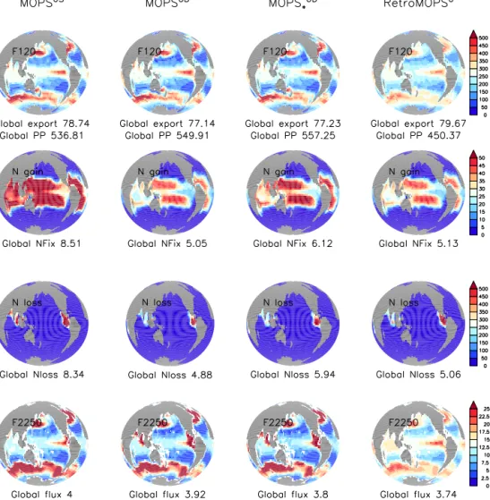
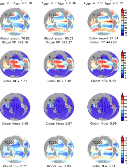
Figure 2.Biogeochemical fluxes of MOPS^◦S, MOPS^◦D, MOPS^◦_∗^Dand RetroMOPS^◦. Top: export production (here: sedimentation at 120 m).

Second row from top: nitrogen fixation. Third row from top: fixed nitrogen loss through pelagic denitrification. Bottom: sedimentation at 2250 m. All fluxes in millimoles of nitrogen per squared metre per year (mmol N m⁻²yr⁻¹). Each sub-panel also gives the global flux in teramoles of nitrate per year (Tmol N yr⁻¹).

exert only a small influence on the fit to global tracer distri- butions (Kriest et al., 2017), this section examines if Retro- MOPS, as a model that parameterises surface biology in a much simpler way, suffices to represent biogeochemical tracer fields. Starting from growth and decay parameters op- timised in MOPS, sensitivity experiments and optimisation search for optimal parameters for DOP production and de- cay, that mimic the surface nutrient turnover of MOPS.

3.2.1 Sensitivity to DOP production and decay

In RetroMOPS fast DOP recycling results in higher primary production, export production and deep organic particle flux, especially in the equatorial upwelling regions (Fig. 4). While this has only a small effect on vertically or globally averaged phosphate concentrations (Figs. 5 and 6), it causes a large underestimate of nitrate in the ocean (Figs. S6 and 6). The

underestimate can be explained by the tight coupling be- tween production, export and denitrification, which leads to higher denitrification and global fixed N loss (Fig. 4), and thus a larger nitrate deficit (Fig. S6) in the eastern equatorial Pacific, in agreement with effects hypothesised and investi- gated by Landolfi et al. (2013).

In contrast, nitrogen fixation is not much affected by DOP turnover rates. The imbalance between nitrogen losses and gains suggests that the models, even after 3000 years of sim- ulation, are not yet in equilibrium, which might be explained by the large spatial scales between regions of fixed nitrogen loss and gain. The divergence increases with higher DOP re- cycling rates (and thus larger denitrification), indicating that there is no unique equilibration timescale for one and the same model, but that it depends on biogeochemical param- eters associated with sinking and remineralisation of organic matter, as observed earlier (Kriest and Oschlies, 2015). The

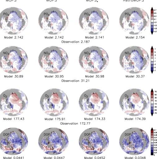
Figure 3. Vertically averaged tracers of MOPS^◦S, MOPS^◦D, MOPS^◦_∗^D and RetroMOPS^◦. Top: phosphate. Second row from top: nitrate.

Third row from top: oxygen. Bottom: DOP. Phosphate (mmol P m⁻³), nitrate (mmol N m⁻³) and oxygen (mmol O₂m⁻³) are expressed as deviation from observations (Garcia et al., 2006a, b), and DOP is given in absolute concentrations (mmol P m⁻³). Each sub-panel also gives the global average tracer concentration (mmol m⁻³).

resulting requirement for long spin-up times for a complete model adjustment, their dependence on biogeochemical pa- rameters and the model’s nonlinearity during spin-up (Kri- est and Oschlies, 2015) complicate model calibration and assessment, in addition to those factors already investigated by Séférian et al. (2016). It emphasises the need for a thor- ough assessment of trade-offs between model complexity and computational demand, and the possibility to examine the parameter space in sufficient detail.

The effect of DOP recycling on oxygen concentrations dif- fers from its effect on nitrate. With fast recycling DOP is remineralised mostly at its place of production, and does not contribute much to oxygen consumption in deep waters (see also Fig. S5). As a consequence, deep oxygen concentrations are high, particularly in the northern North Pacific (Fig. 5), and global average oxygen is overestimated by more than 10 % (Fig. 6). Slow DOP recycling, in contrast, leads to less organic matter remineralisation in well-ventilated waters, but more remineralisation in deep waters. This in turn results in

an underestimate of global mean oxygen of almost 10 % (for λ=0.18 yr⁻¹andλ_s=0 yr⁻¹), which is somewhat surpris- ing, given that production and export in this scenario are the lowest of all simulations (Fig. 4). Overall, the best fit to ob- served inorganic tracer concentrations is achieved with mod- erate DOP recycling (Table 2, Fig. 5).

Most likely because of its fixed inventory, phosphate con- tributes to less than one-third of the misfit function and is quite insensitive to changes in DOP recycling rate (Fig. 6).

Nitrate and oxygen play a larger role for model fit, because their inventory can adapt to changing biogeochemistry. The misfit to nitrate and oxygen increases more or less in concert with their bias (Fig. 6). Therefore, these tracers with their flexible inventory provide some very useful constraints on DOP recycling rates.

Slow DOP recycling increases DOP concentrations at the surface, particularly in the ACC and in the northern North Atlantic (Fig. 5) towards concentrations that exceed the observations (Yoshimura et al., 2007; Raimbault et al.,

Figure 4.As in Fig. 2, but for three sensitivity experiments with model RetroMOPS.

2008; Torres-Valdes et al., 2009; Letscher and Moore, 2015).

Only the simulation with quite fast DOP recycling of λ= 0.72 yr⁻¹ andλ_s=0.36 yr⁻¹ results in reasonable concen- trations of DOP – but at the cost of too-high phosphate con- centrations along these sections, and a too-high global misfit (Table 2), a too-low nitrate and too-high oxygen inventory (Figs. 5 and 6). Therefore, it should be noted that despite the relatively good fit of RetroMOPS^r, it nevertheless suf- fers from a potential mismatch to DOP, which so far is not included in misfit evaluation.

3.2.2 Optimal parameters for DOP cycling in RetroMOPS

All four parameters of RetroMOPS^◦are well constrained by the observations, as indicated by the narrow, almost Gaus- sian distribution around the optimal parameter (Figs. 7, S7, and Table 3). Optimisation reduces the decay rate for surface DOP,λ_s, to almost zero, i.e. in RetroMOPS there seems to be no requirement for fast DOP turnover at the surface, similar

to the results obtained by Letscher et al. (2015). The optimal total remineralisation rate of DOP (λ+λ_s) is about 0.5 yr⁻¹, more than twice as high as the recycling rate estimated by Letscher et al. (2015), but lower than the rates observed by Hopkinson et al. (2002). The optimal fraction of primary pro- duction released as DOP,σ, is 73 % and agrees very well with σ=0.74 obtained by Kwon and Primeau (2006); however, their optimal DOP decay rate was twice as high (1 yr⁻¹).

When optimising a simple biogeochemical model simi- lar to RetroMOPS against observed phosphate, Kwon and Primeau (2006) noted a correlation between DOP produc- tion fraction and decay rate, impeding the simultaneous esti- mation of these parameters. On the contrary, in optimisation RetroMOPS^◦ bothσ and the DOP decay rates seem to be rather well constrained. An analysis of the different compo- nents of the misfit function, similar to Fig. 4 of Kwon and Primeau (2006), helps to resolve this apparent contradiction.

For this, in Fig. 8 the total misfitJand its componentsJ (j ) of Eq. (11), as well as the bias of the best 5 % of all in-

Figure 5.As in Fig. 3, but for three sensitivity experiments with model RetroMOPS.

dividuals are mapped against σ and DOP decay timescale τ =1/(λ+λs).

Note that the analysis depicted in Fig. 8 differs from that of Kwon and Primeau (2006) in several aspects: firstly, their global biogeochemical model was fully equilibrated (due to their direct evaluation of steady state via Newton’s method), whereas simulations of RetroMOPS may still exhibit some drift in nitrogen inventory (see Sect. 3.2.1 and Supplement).

Second, Kwon and Primeau (2006) evaluated model sensi- tivity atb=1, while Fig. 8 displays a region±5 % around optimalb=0.98. Thirdly, Fig. 8 maps only the misfit of so- lutions realised by the optimisation routine, while Kwon and Primeau (2006) analysed the entire parameter space atb=1.

Most important, the misfit function applied here is based on three components, with very different properties and associ- ated timescales (see above), which can be advantageous for parameter estimation.

The misfit to phosphate (Fig. 8, lower left panel) indi- cates an elongated valley in the two-dimensional projection on DOP decay timescaleτ (years) and DOP production frac-

tionσand resembles Fig. 4 of Kwon and Primeau (2006). In- deed, one of the lowest misfits to phosphate is achieved with about the same set of parameters as in Kwon and Primeau (2006), namelyτ≈1,σ ≈0.73. However, nitrate and oxy- gen show a different and, partly, antagonistic pattern: the best fit to observed nitrate is achieved with rather high values of σ≈0.8 andτ between about 1 and 2 years, while the best fit to oxygen is obtained with σ≈0.7 and τ ≈1.5 years.

The superposition of the different components of the misfit function leads to a unique optimum atτ=2 (λ=0.47 and λ_s=0.02) andσ=0.73 (Table 3). Thus, oxygen and nitrate can provide some useful independent information on these parameters.

This can partly be explained by their non-conservative na- ture. As noted in Sect. 3.2.1 the inventory of these tracers may change freely according to model parameterisation. The resulting bias to observations thus adds two important com- ponents to the misfit function, both of which are indepen- dent: while high DOP turnover (as simulated by lowτ) bi- ases nitrate low (Fig. 8, upper mid panel), the same value

Figure 6.Components of the misfit function (J (j) of Eq. 11; upper panels) and model bias (lower panels), projected ontoλ_s andλ. Bias is expressed as(m_j/o_j−1)×100, wherem_j is the global average model tracer, ando_j the average observed tracer, for the three tracers phosphate (j=1; left panels), nitrate (j=2; mid panels) and oxygen (j=3; right panels). An open star indicates the respective lowest misfit or bias.

FrequencyFrequency

FrequencyFrequency

Figure 7.As in Fig. 1, but for optimisation RetroMOPS^◦.

leads to an overestimate of oxygen (Fig. 8, upper right panel;

see also Fig. 6). This behaviour can be explained with the different processes and boundary conditions for the two trac-

ers already noted in Sect. 3.2.1: a high DOP turnover leads to higher fluxes and a tighter coupling of production and den- itrification in upwelling waters, causing a nitrate deficit in the model (see above, and Fig. S6). On the other hand, it re- duces preformed DOP in subducted waters, e.g. the Southern Ocean, thereby decreasing aerobic remineralisation and oxy- gen consumption in these waters on their passage towards, for example, the northern North Pacific. The latter process increases oxygen particularly in deep waters (Fig. S5).

To summarise, including nitrate and oxygen as non- conservative tracers in the misfit function helps to resolve parameters related to DOP production and decay on long timescales. This can be explained by the different pathways of DOP originating from upwelling regions or subducted wa- ter masses in the high latitudes, and is confirmed by the anal- ysis of sensitivity experiments presented in Sect. 3.2.1. How- ever, a better fit to observed phosphate seems to come at the expense of a mismatch to observed DOP concentration. It re- mains to be seen if a simultaneous fit to observed inorganic and organic phosphorus is possible.

3.2.3 Comparison of MOPS and RetroMOPS

The optimal b=0.98 of RetroMOPS^◦ is lower than that of MOPS^◦S and MOPS^◦D. This may be partially explained by the absence of numerical diffusion of detritus in Retro- MOPS. As shown by Kriest and Oschlies (2011), in mod- els that explicitly simulate detritus sinking with an upstream

misfit misfit misfit

Figure 8.Model misfit and relative biasb_j of RetroMOPS^◦, plotted for parameter combinations ofσ and DOP decay timescaleτ, where τ=1/(λ+λs). Relative bias is evaluated byb_j=(m_j/o_j−1)×100, wherem_jdenotes the global mean model concentration of tracerj, ando_j the observed mean. Model misfit is shown as total misfit (J of Eq. 11; upper left) and separated into its components, normalised by o_j (J (j) of Eq. 11; lower panels). The analysis is restricted to all individualsi whosebdiffers less than 5 % from optimal b^∗, i.e.

|b_i/b^∗−1|<0.05. For better visibility some model solutions (≈10) that are outside the range 0.65≤σ≤0.85 and 0.2≤τ≤3 have been omitted from the plot. Open squares denote optimal estimates by Kwon and Primeau (2006, total phosphate constraint), open circles the optimal parameter from this study.

scheme the assumption of homogenous detritus distribution in each vertical grid box causes an additional, usually down- ward transport of detritus. This results in an effectivebwhich is about 10–20 % smaller (corresponding to faster sinking) than the nominally prescribedb. Optimisation of MOPS ac- counts for this additional numerical transport by increasing b(=reducing sinking velocity) by some amount. Therefore, optimal b of MOPS without any influence from numerical diffusion would likely be around 1.1–1.2, i.e. closer to the b=0.98 of RetroMOPS^◦. Considering this effect, the op- timalb of MOPS^◦D and, in particular, RetroMOPS^◦ agrees with the optimal value ofb=1 found by Kwon and Primeau (2006).

Despite its generally lower fluxes, fixed nitrogen loss in the eastern equatorial Pacific is higher in RetroMOPS^◦than in MOPS^◦D(Fig. 2), resulting in a nitrate deficit in this region.

Likely, the instantaneous remineralisation of sinking material inherent in the direct flux parameterisation of RetroMOPS causes a tighter spatial coupling between production, sink- ing, remineralisation and upwelling (see also Sect. 3.2.1).

It has been suggested earlier that the production of slowly

degradable organic matter above upwelling regions and/or oxygen minimum zones may help to decouple these pro- cesses and avoid a runaway effect of nitrate loss (Landolfi et al., 2013; Dietze and Loeptien, 2013). The very low opti- mal value for surface DOP turnoverλs found in this study, and also in the study by Letscher et al. (2015), supports this finding.

Simulated biogeochemical fluxes of RetroMOPS^◦are gen- erally lower than those of MOPS^◦D, and their horizon- tal pattern is less pronounced (Fig. 2). This likely arises from the prescribed, constant phytoplankton concentration of RetroMOPS^◦, which mutes biogeochemical dynamics in productive regions of the high latitudes and upwelling ar- eas. Because RetroMOPS^◦ applies the same parameters as MOPS^◦D for oxidant-dependent processes, its global fixed nitrogen loss and gain is comparable to that of the more com- plex model.

The total misfit to observed dissolved tracer concentra- tions of RetroMOPS^◦is only about 4 % higher than that of MOPS^◦D, suggesting that even the simple RetroMOPS can perform almost as well as MOPS with respect to annual mean