A revised global estimate of dissolved iron fl uxes from marine sediments
A. W. Dale1, L. Nickelsen1, F. Scholz1, C. Hensen1, A. Oschlies1, and K. Wallmann1
1GEOMAR Helmholtz Centre for Ocean Research Kiel, Kiel, Germany
Abstract
Literature data on benthic dissolved iron (DFe)fluxes (μmol m2d1), bottom water oxygen concentrations (O2BW,μM), and sedimentary carbon oxidation rates (COX, mmol m2d1) from water depths ranging from 80 to 3700 m were assembled. The data were analyzed with a diagenetic iron model to derive an empirical function for predicting benthic DFefluxes:DFe flux¼γtanhOC2BWOXwhereγ(= 170μmol m2d1) is the maximumflux for sediments at steady state located away from river mouths. This simple function unifies previous observations that COXand O2BWare important controls on DFefluxes. Upscaling predicts a global DFe flux from continental margin sediments of 109 ± 55 Gmol yr1, of which 72 Gmol yr1is contributed by the shelf (<200 m) and 37 Gmol yr1by slope sediments (200–2000 m). The predicted deep-seaflux (>2000 m) of 41 ± 21 Gmol yr1is unsupported by empirical data. Previous estimates of benthic DFefluxes derived using global iron models are far lower (approximately 10–30 Gmol yr1). This can be attributed to (i) inadequate treatment of the role of oxygen on benthic DFefluxes and (ii) improper consideration of continental shelf processes due to coarse spatial resolution. Globally averaged DFe concentrations in surface waters simulated with the intermediate-complexity University of Victoria Earth System Climate Model were a factor of 2 higher with the new function. We conclude that (i) the DFeflux from marginal sediments has been underestimated in the marine iron cycle and (ii) iron scavenging in the water column is more intense than currently presumed.
1. Introduction
Iron (Fe) is a regulating micronutrient for phytoplankton productivity and the efficiency of the biological pump over large areas of the ocean [Martin and Fitzwater, 1988;Martin, 1990; Moore and Doney, 2007;Boyd and Ellwood, 2010]. Natural iron fertilization by enhanced dust inputs is believed to have contributed to lower CO2 levels during the Last Glacial Maximum [Martin, 1990; Sigman and Boyle, 2000]. Understandably, therefore, global circulation models with a focus on Fe have often considered dissolution from dust to be the major external source of dissolved iron to the surface ocean [Archer and Johnson, 2000;Aumont et al., 2003;Parekh et al., 2004]. The atmospheric, dissolvable iron input is around 10 Gmol yr1or less, yet is highly uncertain due to the poorly constrained solubility of particulate iron [Jickells et al., 2005; Luo et al., 2008;
Mahowald et al., 2005;Galbraith et al., 2010;Misumi et al., 2014;Nickelsen et al., 2015].
More recently, continental margin sediments have been shown to be important sources of dissolved iron (DFe) to the coastal ocean and beyond [Elrod et al., 2004;Lohan and Bruland, 2008;Cullen et al., 2009;Severmann et al., 2010;Jeandel et al., 2011;John et al., 2012;Conway and John, 2014]. Most global iron models now include an explicit sediment source of DFe, albeit with very different parameterizations. For instance, benthic DFefluxes have been described using afixed or maximumflux at the seafloor [Moore et al., 2004;Aumont and Bopp, 2006;Misumi et al., 2014]. Others used the empirical relationship between DFeflux and benthic carbon oxidation rates (COX) proposed byElrod et al. [2004] [Moore and Braucher, 2008;Palastanga et al., 2013]. In recognition that DFefluxes from marine sediments are enhanced under oxygen-deficient bottom waters [McManus et al., 1997;Lohan and Bruland, 2008;Severmann et al., 2010], some workers opted for an oxygen
“switch”[Galbraith et al., 2010; Nickelsen et al., 2015]. Here, all particulate iron that falls to the seafloor is returned to the water column as DFe if bottom water oxygen concentration (O2BW) falls below a predefined threshold. Given the lack of consensus of how benthic iron should be described in models, the magnitude of this source is only vaguely constrained at 8–32 Gmol yr1[Jickells et al., 2005;Galbraith et al., 2010; Misumi et al., 2014; Nickelsen et al., 2015; Tagliabue et al., 2014]. This uncertainty is very likely propagated to the parameterization of the DFe source/sink terms in the water column, which themselves are very poorly understood [Nickelsen et al., 2015]. Thus, there is a real need to better constrain DFe sources and sinks in the ocean.
Global Biogeochemical Cycles
RESEARCH ARTICLE
10.1002/2014GB005017
Key Points:
•Global dissolved ironflux from margin sediments of 109 ± 55 Gmol yr1
•Benthic dissolved ironflux has been underestimated in the marine iron cycle
•Iron scavenging rates in water column probably higher than currently presumed
Supporting Information:
•Text S1, Figure S1, and Tables S1–S5
Correspondence to:
A. W. Dale, adale@geomar.de
Citation:
Dale, A. W., L. Nickelsen, F. Scholz, C. Hensen, A. Oschlies, and K. Wallmann (2015), A revised global estimate of dissolved ironfluxes from marine sediments,Global Biogeochem. Cycles, 29, 691–707, doi:10.1002/
2014GB005017.
Received 15 OCT 2014 Accepted 2 APR 2015
Accepted article online 7 APR 2015 Published online 28 MAY 2015
©2015. American Geophysical Union. All Rights Reserved.
While there is little disagreement that both O2BWand COXare important factors for predicting DFefluxes, a unifying paradigm has so far not been proposed in a quantitative and empirical fashion. The oxygen threshold used byGalbraith et al. [2010] andNickelsen et al. [2015] is an advance in the right direction, but the threshold concentration is somewhat arbitrary and not well justified empirically. In this study, we reanalyze the available literature data at sites where benthic DFefluxes, O2BW, and COXhave been reported. Our prime objective is to derive a simple algorithm to predict DFefluxes from marine sediments at the global scale based on O2BW and COXas the two key controlling variables. We then analyze the impact of this source on DFe distributions in ocean surface waters by coupling the algorithm to the intermediate-complexity University of Victoria Earth System Climate Model (UVic ESCM). Wefind that the sedimentary DFe source may be several times higher than current estimates suggest, implying that scavenging in the water column is currently too weak in global iron models and that the residence time of iron in the ocean is shorter than assumed previously.
2. Data Acquisition and Evaluation
Benthic ironfluxes were compiled from the literature along with reported O2BWand COX(Table 1). In these studies, the water samples for iron analysis were filtered (0.45μm), acidified, and analyzed for the total dissolved fraction using various analytical methodologies (see Table 1). Only fluxes measured using non-invasive benthic chambers were considered. DFefluxes derived from pore water gradients often do not correlate with in situfluxes due to processes at the sediment-water interface operating over spatial scales smaller than the typical centimeter-scale sampling resolution [e.g., Homoky et al., 2012]. Furthermore, enhanced DFeflux to the bottom water byflushing of animal burrows (bioirrigation) is also not captured by pore water gradients. We note, however, that benthic DFefluxes determined using chambers may also suffer from artifacts due to oxidative losses and scavenging onto particles [e.g.,Severmann et al., 2010]. In this study, we make no attempt to reevaluate the published data with regards to these aspects and the reported benthic DFefluxes are used.
Almost all data where DFefluxes, O2BW, and COXhave been measured simultaneously originate from the Californian shelf and slope [McManus et al., 1997;Berelson et al., 2003;Severmann et al., 2010]. These data cover a wide range of COXand O2BWfrom severely hypoxic (~3μM) to normal oxic (>63μM) conditions.
DFefluxes range from<0.1μmol m2d1on the slope to 568μmol m2d1in the San Pedro Basin. High fluxes of 332μmol m2d1were also measured on the Oregon margin close to river mouths [Severmann et al., 2010]. Absent from the Californian data are DFefluxes under anoxic conditions. In situ fluxes are available for anoxic areas of the Baltic and Black Seas [Friedrich et al., 2002;Pakhomova et al., 2007]. Yet these are not included in our database because supporting COX data are unfortunately lacking. We therefore supplemented the database withfluxes from the Peruvian oxygen minimum zone where bottom waters on the shelf and upper slope are predominantly anoxic [Noffke et al., 2012]. The highest DFeflux in Table 1. Literature Data on Benthic DFe Fluxes
Region
Water Deptha (m)
O2 (μM)
COX (mmol m2d1)
DFe Flux
(μmol m2d1) Remarks
Californian margin and Borderland Basinsb
100–3700 8–138 0.3–7.3 0.02–48 Highestfluxes with shallow oxygen penetration depths Monterey Bay (California)c 100 101–185 6.9–14.7 1.3–10.8 Interannual and intraannual variability
at a single station Oregon-California shelf and Californian
Borderland Basinsd
90–900 3–153 2–23 12–568 Highfluxes for Eel River mouth and San Pedro and Santa Monica Basins, temporal variability Peruvian margine 95–400 <d.l 2.4–7.7 11–888 Highestflux measured for an open margin setting
aDepth range where the data were collected.
bMcManus et al. [1997]: Total dissolved iron determined by chemiluminescence. Positivefluxes only (= out of sediment). Negativefluxes are<0.5μmol m2d1 and ignored in this study. COXwas determined fromΣCO2fluxes corrected for carbonate dissolution.
cBerelson et al. [2003]: Total dissolved iron determined byflow injection analysis with chemiluminescence detection. COXwas determined fromΣCO2fluxes corrected for carbonate dissolution.
dSevermann et al. [2010]: Total dissolved iron determined by inductively coupled plasma mass spectrometry. DFefluxes of 421 to 568μmol m2d1were reported for the San Pedro and Santa Monica Basins compared to only 13–18μmol m2d1measured previously at the same sites (reported byElrod et al.
[2004]). COXwas determined fromΣCO2fluxes without correction for carbonate dissolution.
eNoffke et al. [2012]: Total dissolved iron determined by inductively coupled plasma mass spectrometry. COXwas determined as the HCO3flux from pore water total alkalinity gradients and showed very good agreement with numerical modeling results [Bohlen et al., 2011].
our database was measured here (888μmol m2d1). In this study, we define anoxia as O2concentrations below the detection limit of the Winkler titration, approximately 3μM.
Thefinal database includes 81 data points where DFeflux, O2BW, and COXdata have been reported for the same site. DFefluxes and COXwere taken as the reported mean values plus error (where given) determined from multiple chambers during the same deployment. Hence, the actual number of individual DFefluxes is much greater than 81. In total, 25fluxes are from shelf settings (≤200 m), 40 are from the slope (>200–2000 m), and 16 are from deeper waters down to 3700 m. The deep sea is thus underrepresented in the database compared to the continental margin.
0 50 100 150 200
Bottom water O2 (µM) 0.01
0.1 1 10 100 1000
Individual sites (0-200 m) Individual sites (200-1000 m) Mean measured (O2 < 3 µM) Mean measured (O2 > 3-20 µM) Mean measured (O2 > 20-63 µM) Mean measured (O2 > 63 µM)
0 5 10 15 20 25
Carbon oxidation rate (mmol m-2 d-1) 0.01
0.1 1 10 100 1000
DFe flux (µmol m-2 d-1 )DFe flux (µmol m-2 d-1 )
Individual sites
Mean measured (O2 < 3µM)) Mean measured (O2 >3-20 µM) Mean measured (O2 >20-63 µM) Mean measured (O2 >63 µM) Mean modelled (O2 < 3 µM)) Mean modelled (O2 >3-20 µM) Mean modelled (O2 >20-63 µM) Mean modelled (O2 >63 µM) Shelf
Slope
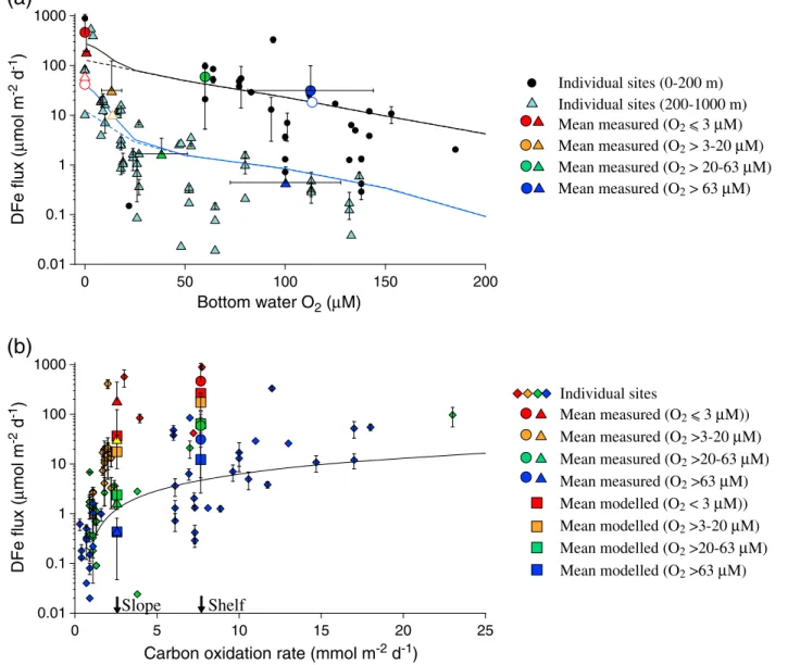
Figure 1.(a) Measured DFefluxes versus bottom water O2. Black circles and light blue triangles correspond to individual sites with COX>4 (≈shelf) and
<4 mmol m2d1(≈slope), respectively. The larger colored symbols are the mean DFefluxes and O2concentrations within each binned range of O2(error bars are standard deviations), where circles and triangles denote shelf and slope, respectively. The large white symbols with colored outlines show the binned data without the fourfluxes>300μmol m2d1(San Pedro Basin, Santa Monica Basin, Eel River shelf, and Peruvian shelf). The black and blue curves are modeledfluxes for the shelf and slope, respectively; solid curves = standard model and dashed lines = standard model with no decrease in faunal activity at low O2BW. (b) Measured DFefluxes versus COXcolor coded according to O2BW(diamonds). The large circles (shelf) and triangles (slope) are the measured binned data from Figure 1a plotted for the shelf and slope values of COX(indicated on thexaxis). The mean modeledfluxes for each O2BWinterval are the corresponding colored squares. The curve is the regression of Elrod et al. [2004]: DFe = 0.68 × COX0.5, based on data published byMcManus et al. [1997] andBerelson et al. [2003]. Error bars for the individual sites in Figures 1a and 1b are taken from the literature where reported (Table 1). Error bars on COXare not shown for clarity.
Atfirst glance, defining any relationship between DFeflux, O2BW, and COX seems like an impossible task (Figure 1). DFefluxes scatter over many orders of magnitude for any given O2BWor COX. The apparent dependence of DFeflux on O2BW, as observed in the data set ofSevermann et al. [2010], is much more tenuous when data from all studies are considered collectively. The linear relationship between DFeflux (inμmol m2d1) and COX(in mmol m2d1) proposed byElrod et al. [2004] does seem to broadly apply (DFe = 0.68 × COX0.5), although DFefluxes>10μmol m2d1for low COXare not well represented by that model (Figure 1b).
In order to understand the scatter in these plots, wefirst organized the individualfluxes into two groups depending on whether the COX was above or below 4 mmol C m2d1. This definition is not arbitrary;
it represents the COX at the shelf break (approximately 200 m) where a sharp gradient change in total benthic O2 uptake occurs [Andersson et al., 2004]. Above this depth (i.e., on the shelf ), COX increases to >20 mmol m2d1, whereas on the slope it declines much more gradually to approximately 1 mmol m2d1 or less at 3000 m [Burdige, 2007]. Although we recognize that COX does not strictly correlate with water depth, the overall relationship is clear enough [see Burdige, 2007] that we can collectively term the sites above and below the COXthreshold as shelf and slope, respectively.
In a second step, the DFefluxes were binned into discrete O2BWintervals: anoxic (O2BW≤3μM), severely hypoxic (>3μM<O2BW≤20μM), weakly hypoxic (>20μM<O2BW≤63μM), and normal oxic (O2BW>63μM). Two of these boundaries were chosen based on strict (i.e., anoxia, that is, below detection limit) or more consensual definitions (i.e., hypoxia = O2<~63μM). The 20μM boundary is somewhat subjective. We chose this value becauseElrod et al. [2004] noted that their DFe-COXcorrelation did not capture ironfluxes at sites with O2BW concentrations below this value. It may well be that this concentration represents a tipping point beyond which large changes in DFeflux occur due to alterations in respiration pathways and/or faunal regime shifts [Levin and Gage, 1998]. We will revisit this idea later.
Following these criteria, the data broadly show that DFeflux correlates inversely with increasing O2BWand decreasing COX. High DFe fluxes on the shelf (circles in Figure 1a) are clearly distinguishable from the much lower fluxes on the slope (triangles). For the slope setting, low DFe fluxes of 1.3 and 0.4μmol m2d1are found for the weakly hypoxic and oxic intervals, respectively, whereas a pronounced increase to 36 and 188μmol m2d1 is associated with the severely hypoxic and anoxic intervals (respectively). A very similar trend emerges for the shelf with a high-end flux of 465μmol m2d1 in anoxic shelf settings. However, there is a large uncertainty associated with these numbers due to (i) few data available for anoxic and hypoxic sites on the shelf and (ii) bias toward the highfluxes measured in the San Pedro and Santa Monica Basins and on the Peru and Eel River shelves. Excluding these four points with DFe fluxes >300μmol m2d1 considerably reduces the binned values for anoxic and severely hypoxic waters (open symbols in Figure 1a). Furthermore, it is also not clear if the highfluxes on the shelf truly reflect higher COXor whether this simply reflects the fact that most organic matter is deposited on the shelf along with iron-rich terrestrial material. Consequently, in the following section we use a diagenetic model to identify the factors regulating benthic iron fluxes and provide a mechanistic understanding of the emerging trends in Figure 1.
3. Benthic Iron Model
A vertically resolved 1-D reaction-transport model was used to simulate the coupled C, N, Fe, Mn, and S cycles in the upper 30 cm of sediments. Our aim is to calculate benthic DFefluxes in representative shelf (0–200 m) and upper slope (200–1000 m) environments for the observed range of O2BW(1–200μM) and compare these to the measured data in Figure 1. Water depths of 100 m and 600 m (respectively) were chosen based on conventional hypsometric intervals [Menard and Smith, 1966]. In the model, solids are transported dynamically by sediment accumulation and by bioturbation in the upper mixed surface layer where metazoans mainly reside. Solutes are also affected by molecular diffusion and bioirrigation, the latter describing the nonlocal exchange of seawater with pore water by burrowing fauna. The model is described fully in the supporting information. It is based on previous empirical diagenetic models, and for greater transparency we have formulated the biogeochemical reactions and parameters in line with these studies [e.g.,Van Cappellen and Wang, 1996;Wang and Van Cappellen, 1996;Berg et al., 2003;Dale et al., 2009, 2013].
The parameterization of key transport processes, boundary conditions, and kinetic parameters was achieved using global empirical relationships where possible (Table 2). The sedimentation rate and surface bioturbation coefficient were calculated on the basis of water depth [Burwicz et al., 2011;Middelburg et al., 1997]. Similarly,Burdige[2007] compiled a database of sediment COXfor the same water depth intervals as used here. As a first approximation, this was assumed to be equal to the total rain rate of particulate organic carbon (POC) to the seafloor since less than 10% of organic matter reaching the ocean floor is ultimately preserved in marine sediments [Hedges and Keil, 1995]. Bioirrigation coefficients were calculated following the procedure ofMeile and Van Cappellen[2003]. In line with other models, irrigation of Fe2+was lowered relative to other solutes due to its high affinity to oxidation on burrow walls [Berg et al., 2003;Dale et al., 2013]. Fluxes of total iron oxides were defined according to the bulk sedimentation rate (Table 2).
Due to the general scarcity of data from sediments underlying oxygen-deficient waters, these global relationships apply to normal oxic conditions. Yet the bioirrigation and bioturbation coefficients cannot be treated as constant parameters in the simulations due to the dependency of metazoans on oxygen. Faunal activity levels under low O2are not well documented, but the rate and intensity of bioturbation and irrigation are probably lower [Diaz and Rosenberg, 1995;Middelburg and Levin, 2009]. The bioirrigation and bioturbation coefficients were thus multiplied by a factor (f) that mimics the reduction in faunal activity at low O2BW (Table 2). Specifically, the maximum bioirrigation and bioturbation rates are reduced by 50% when O2BWis at the level where shifts in faunal community structure occur (approximately 20μM) [Levin and Gage, 1998].
Bioirrigation and bioturbation rates are depressed even further at lower O2BW, in line withfield observations [Dale et al., 2013]. The model sensitivity to constant animal mixing rates for all O2BWlevels is shown below.
Table 2. Key Model Parameters Used in the Simulation of the Shelf and Slope Sedimentsa
Shelf Slope Source
Representative water depth (m)b 100 600 Menard and Smith[1966]
Temperature of the bottom water (°C) 10 8 Thullner et al. [2009]
Sediment accumulation rate,ωacc(cm kyr1) 100 16 Burwicz et al. [2011]
POC rain rate,FPOC(mmol m2d1)c 9.4 3 Burdige[2007]
Total iron oxide (FeT) rain rate,FFeT(μmol m2d1)d 1840 290 This study Dissolved oxygen concentration in seawater, O2BW(μM)e Variable Variable This study
Dissolved ferrous iron concentration in seawater 0 0 This study
Rate constant for aerobic Fe2+oxidation,k13(M1yr)f 5 × 10⁸ 5 × 10⁸ Various Bioturbation coefficient at surface,Db(0) (cm2yr1)g 28 ·f 18 ·f Middelburg et al. [1997]
Bioturbation halving depth,zbt(cm2yr1) 3 3 Teal et al. [2008]
Bioirrigation coefficient at surface,α(0) (yr1)g,h 465 ·f 114 ·f Meile and Van Cappellen[2003]
Bioirrigation attenuation coefficient,zbio(cm)i 2 0.75 This study Average lifetime of the reactive POC components,a(yr)j 3 × 10⁴ 3 × 10⁴ Boudreau et al. [2008]
Shape of gamma distribution for POC mineralization,υ()j 0.125 0.125 Boudreau et al. [2008]
aThe complete model is described in the supporting information.
bThe mid-depth of the shelf (0–200 m) and upper slope (200–1000 m) according toMenard and Smith[1966].
cTable 4 inBurdige[2007], based on his compilation of benthic carbon oxidation rates.
dFluxes of total particulate iron oxide (FeT) to the sediment were based on the Fe content in average sedimentary rock (~5%) [Garrels and Mackenzie, 1971] which is similar to Fe content in red clays [Glasby, 2006]. The total Feflux was calculated using the equation 0.05 ·ωacc· (1φ(L)) ·ρs/AWwhereφ(L) is the porosity of compacted sediment (0.7),ρsis the dry sediment density (2.5 g cm3), andAWis the standard atomic weight of iron (55.8 g mol1). Fifty percent of thisflux is unreactive [Poulton and Raiswell, 2002], and the other 50% is divided equally among FeHR, FeMR, and FePR(see text).
eValues tested in the model are 1, 2, 5, 10, 15, 25, 50, 100, and 200μM.
fVan Cappellen and Wang[1996],Wang and Van Cappellen[1996],Berg et al. [2003], and others. See supporting information for reaction stoichiometry and kinetics.
gA dimensionless factor that scales the bioturbation and bioirrigation coefficients to O2BW(μM) isf. It is equal to 0.5 + 0.5 · erf((O2BWa)/b), where erf is the error function anda(20μM) andb(12μM) are constants that define the steepness of decline offwith decreasing O2BW.
hMeile and Van Cappellen[2003] calculated the average bioirrigation coefficient in surface sediments (α, year1) based on total sediment oxygen uptake and bottom water O2. As afirst approximation, sediment oxygen uptake was assumed to be equal toFPOC.α(0) was calculated fromαfollowingThullner et al. [2009] for a bottom water O2concentration of 120μM which is representative of shelf and slope environments. Irrigation of Fe2+was scaled to 20% of that for the other solutes due to its high affinity for oxidation on burrow walls.
iThe depth of the sediment affected by irrigation on the shelf was adjusted to coincide with the depth of the biotur- bation zone (approximately 7 cm).
jA full description of POC degradation kinetics is given in the supporting information.
Continuum kinetics for describing POC degradation is a key aspect of the model [Middelburg, 1989;Boudreau and Ruddick, 1991]. This approach captures the temporal evolution of organic matter reactivity, as opposed to multi-G models that predefine afixedfirst-order decay constant of one or more carbon fractions [Westrich and Berner, 1984]. However, continuum models cannot be readily applied to bioturbated sediments due to random mixing of particles of different ages by animals [Boudreau and Ruddick, 1991]. Thus, we developed a procedure for approximating the continuum model in bioturbated sediments by defining multiple (14) carbon pools based on the initial distribution of carbon reactivity (see supporting information). This distribution is defined by two parameters: the average lifetime of the reactive components,a(yr), and the distribution of POC reactivity, υ () (Table 2). Low υ values indicate that organic matter is dominated by refractory components, whereas higher values correspond to a more even distribution of reactive types. Similarly, organic matter characterized by lowawill be rapidly degraded below the sediment-water interface, whereas a highaimplies less reactive material that is more likely to be buried to deeper sediments. While we can expect some regional differences in these parameters, we used values corresponding to fresh organic matter to shelf and slope settings [Boudreau et al., 2008]. This is a reasonable, but not entirely robust, assumption given relatively rapid particulate sinking rates in the water column [Kriest and Oschlies, 2008].
A comprehensive iron cycle is included. The reactivity of particulate iron (oxyhydr)oxides (hereafter Fe oxides) was defined according to the widely employed classification based on wet chemical extraction methods [Canfield et al., 1992;Raiswell and Canfield, 1998; Poulton et al., 2004]. Reactive Fe oxides can be broadly defined as highly reactive (FeHR), moderately reactive (FeMR), or poorly reactive (FePR). FeHR has a half-life of<1 yr and represents iron contained within amorphous and reactive crystalline oxides (ferrihydrite, goethite, lepidocrocite, and hematite), pyrite, and acid volatile sulfides, plus a small fraction of iron in reactive silicates [Canfield et al., 1992;Raiswell and Canfield, 1998]. FePRhas a half-life of at least 105years and represents iron released from a wide range of reactive silicates and magnetite. FeMR comprises all the iron with a reactivity intermediate between FeHR and FePR (i.e., magnetite and reactive silicates) with a half-life of 102years. An additional terrigenous detrital iron fraction, representing Fe bound within silicate minerals (FeU), is essentially unreactive on early diagenetic time scales and constitutes about half of all sedimentary iron underlying oxic waters [Poulton and Raiswell, 2002]. The model simulates all four of these fractions, defined chemically as Fe(OH)3. The Fe cycle involves a number of oxidation-reduction pathways (see supporting information). These include authigenic precipitation of FeHRvia aerobic and anaerobic oxidation of ferrous iron; processes that constitute an efficient geochemical barrier against DFe release from the sediment [McManus et al., 1997;Berg et al., 2003]. Reactive Fe oxides can be reduced by dissolved sulfide according to the reaction kinetics proposed byPoulton et al. [2004]. FeHRis also consumed by dissimilatory iron reduction (DIR), whereas the other phases are too crystalline (unreactive) to be of benefit to iron-reducing bacteria [Weber et al., 2006].
Nonreductive dissolution of iron has also been proposed to be a dominant source of benthic iron on continental margins that display low rates of reductive Fe dissolution [Radic et al., 2011; Jeandel et al., 2011; Homoky et al., 2013; Conway and John, 2014]. However, this process has not been described mechanistically and is not considered in our model at this point in time. FeHRfurther undergoes aging into more crystalline FeMR[Cornell and Schwertmann, 1996]. The iron module also includes iron monosulfide (FeS) and pyrite (FeS2) precipitation, the latter via the H2S pathway (Berzelius reaction) and by reaction with elemental sulfur, S0 (Bunsen reaction) [Rickard and Luther, 2007]. FeS and FeS2 can be oxidized aerobically, whereas S0can disproportionate to sulfate and sulfide.
The model was coded and solved using the method of lines with MATHEMATICA 7.0 assuming a diffusive boundary layer of 0.04 cm thickness at the sediment-water interface [Boudreau, 1996]. Further details on the model solution can be found in the supporting information.
4. Model Results
The model reproduces the trend of higher DFefluxes with decreasing O2BW(Figure 1a) and increasing COX (Figure 1b). The absolute magnitude of the modeledfluxes for the shelf and slope settings depends on the water depths chosen to represent these environments, meaning that thefluxes are not as rigidly defined as implied in the plots. The modeled DFefluxes for each O2BWinterval in the anoxic and severely hypoxic intervals are underestimated. Yet with the exception of the anoxic shelf, removing the four fluxes
>300μmol m2d1improves the agreement with the model (open symbols, Figure 1a). The anoxic shelfflux is tenuous because only two data points are available here.
As O2BWincreases, a larger fraction of POC is respired by O2at the expense of other electron acceptors, principally sulfate (Figure 2a). DIR accounts for less than 2% of POC respiration under all O2BWconditions on the shelf and less than 0.2% on the slope. Nonetheless, DIR constitutes the largest source of DFe for anoxic and hypoxic settings (Figure 2b). At higher O2BW, reduction of iron oxides by sulfide becomes more important. Thisfinding is counterintuitive because sulfidic reduction is expected to be less pronounced as O2BWincreases. It can be explained by the increase in bioturbation which mixes labile iron oxide below the surface sediment where POC mineralization rates are highest (Figure 2d). This results in a less pronounced Figure 2.Simulated rates for the shelf environment for each oxygen regime are indicated at the top of thefigure (Figures 2a–2c). (a) POC mineralization pathways. Fe and Mn oxide reduction rates are<0.1 mmol m2d1and not indicated. (b) DFe sources. Iron sulfide oxidation is negligible and only shown for the oxic setting. (c) DFe sinks. Oxidation by NO3and irrigation are negligible and not shown. Aerobic oxidation of ferrous iron in the anoxic setting is zero and also not shown. The total sum of sinks (= sum of sources) is shown underneath the lower pie charts. (d) Sediment depth profiles of POC mineralization rate (RPOC) and dissimilatory iron reduction (DIR) in mmol cm3yr1of C and dissolved ferrous iron and oxygen concentration inμM for representative O2BWin each interval (note different depth scales). Total fluxes on the slope are lower, but the pathways are qualitatively similar.
DIR peak and a greater likelihood that iron oxide is instead reduced by sulfide deeper down. In these subsurface horizons, iron undergoes repeated redox cycling (Figures 2b and 2c) whereby DFe is oxidized to Fe(III), mainly by Mn(IV), and then regenerated when the authigenic iron oxide is again reduced by sulfide or organic matter [e.g., Wang and Van Cappellen, 1996]. This tends to increase the apparent total rate of iron sources (or sinks), from 595μmol m2d1 under anoxia to 757μmol m2d1 under weakly hypoxic conditions, even though the totalflux of particulate iron to the sediment is the same in all cases.
Under near-anoxic conditions, almost half of all DFe is lost to the water column (Figure 2c). A sink switching effect takes place with higher O2BW, whereby DFe oxidation increases at the expense of benthic DFe loss, thereby leading to greater retention of DFe. DFefluxes fall sharply when bottom waters transition from severe to weak hypoxia, which is reflected in the field observations by the increase in DFe fluxes when O2BW<20μM (Figure 1). This concentration may represent a tipping point, beyond which sediments become highly efficient at retaining the iron deposited on the sediment surface. In this regard, it is noteworthy that the boundary between surface sediments that are enriched and depleted in Fe in the Peruvian oxygen minimum zone is located exactly where bottom oxygen concentrations rise above 20μM [Scholz et al., 2014a].
The impact of O2BWon DFefluxes is illustrated more graphically by the DFe pore water concentrations in Figure 2d. Under very low O2BW, the DFe concentration gradient at the sediment-water interface is extremely sharp, which drives a large flux across the diffusive boundary layer. In this case, O2 barely penetrates the sediment and acts as a poor geochemical barrier to DFeflux [McManus et al., 1997]. Under weakly hypoxic conditions, O2BWpenetrates deeper leading to a more efficient oxidative sink for DFe. The resulting DFe concentration gradient in the uppermost millimeters is markedly shallower and theflux to the bottom water much smaller. Finally, under normal oxic conditions, the DFe peak is spatially separated from the surface by several centimeters and only a very weak DFeflux is predicted.
We propose that the DFeflux tipping point is related to sediment ventilation by burrowing animals. The impact of irrigation in our model is demonstrated by the dashed curves in Figure 1a which show that DFe fluxes are much lower on the shelf and slope if faunal activity is unaffected by low O2BW. This conflicts withElrod et al. [2004], who suggested that DFefluxes were enhanced by bioirrigation in Monterey Bay sediments (O2BW>100μM). Yet the importance of bioirrigation in mitigating DFefluxes is supported by previous observations. First, mesocosm experiments showed that burrowing fauna increase iron retention due to rapid immobilization of DFe as particulate iron oxide phases on burrow walls [Lewandowski et al., 2007]. These results have been reproduced using bioirrigation models that employ empirically derived rate constants for aerobic DFe oxidation [Meile et al., 2005]. Second, bottom water DFe concentrations in the later stages of sediment incubations increase quasi-exponentially concomitant with dissolved oxygen depletion [Severmann et al., 2010]. This has been attributed to the loss of the surface oxidized layer on the walls of animal burrows as well as a reduced rate of DFe oxidation in oxygen-depleted chamber waters.
More generally, DFefluxes are low in sediments bearing a surface oxidized layer [McManus et al., 1997].
Clearly, then, in addition to COX, DFe fluxes show a strong dependence on O2BW, especially for concentrations below 20μM. In the following section, we derive a function based on both these variables to predict DFefluxes from sediments.
Table 3. Input Parameters and Boundary Conditions Used in the Standard Model and for the Sensitivity Analysisa Standard Model Sensitivity Analysis
Representative water depth (m) 350 350
Sediment accumulation rate,ωacc(cm kyr1) 60 60
POC rain rate,FPOC(mmol m2d1) 6.2 0.5–15b
Total iron oxide (FeT) rain rate,FFeT(μmol m2d1) 1110 1110
Dissolved oxygen concentration in seawater, O2BW(μM) 120 1–200c
Bioturbation coefficient at surface,Db(0) (cm2yr1) 23 ·f 23 ·f
Bioirrigation coefficient at surface,α(0) (year1) 290 ·f 290 ·f
Bioirrigation attenuation coefficient,zbio(cm) 1.4 1.4
aModel parameters that are unchanged from Table 2 are not listed.
bValues tested (in mmol m2d1) are 0.5, 1, 2, 4, 6, 8, 10, 12, 14, and 16, which are equivalent to COXof 0.4, 0.8, 1.7, 3.3, 5.0, 6.6, 8.3, 9.9, 11.6, and 13.2.
cValues tested are 1, 2, 5, 10, 15, 25, 50, 100, and 200μM.
5. Derivation of a Predictive Function for Benthic Iron Fluxes
An empirical function for predicting benthic DFe fluxes from COX and O2BW was derived using a more detailed sensitivity analysis. This was based on a standardized model defined by the average parameter values of the shelf and slope settings (Table 3). A series of model runs was executed where organic matter rain rate and O2BW were varied between 0.5–16 mmol m2d1 and 1–200μM, respectively. The corresponding COX for these rain rates is 0.4–13.2 mmol m2d1. These ranges are characteristic of the sites in Table 1 and much of the seafloor in general. Although rain rate and O2BWwere the only two model aspects to be varied directly, the bioturbation and bioirrigation coefficients were dependent on O2BW, as described previously. This avoids anomalous scenarios, such as high bioirrigation at sites with low benthic respiration.
The dependence of DFe flux on O2BW for constant values of COX is shown in Figure 3a. DFe flux increases with decreasing O2BWfor all COX, with a tipping point centered at around 20μM, as observed previously. Furthermore, sedi- ments release more iron as COX increases due to higher rates of aerobic carbon respiration at the expense of DFe oxidation.
Benthic DFeflux also responds strongly to small increases in COXwhen O2BWis below approximately 10μM (Figure 3b). The pronounced peak in DFe centered at COX= 2 mmol m2d1originates from high DIR rates close to the sediment surface (cf. Figure 2d). The subsequent dip in DFe flux when COX~ 4 mmol m2d1 signifies sequestration of iron into sulfide minerals as sulfate reduction rates increase. DFefluxes then gradually increase again with higher COXas in Figure 3a. These results demonstrate that COXis itself an important factor to consider for predicting DFefluxes, in addition to the totalflux of labile particulate iron (see below).
The sensitivity analysis supports observations that COXacts on DFeflux in an opposite way to O2BW[Elrod et al., 2004;Severmann et al., 2010]. Hence, we derived a predictive function for DFefluxes (inμmol m2d1) to reflect this behavior:
DFe flux¼γtanh COX
O2BW
(1)
where COXis in mmol m2d1and O2BWis inμM. The maximumflux that can escape the sediment for a given Fe content and reactivity isγ. In our simulations, this is predicted to be 170μmol m2d1.
The function is an example of a 0-D vertically integrated sediment model following the criteria ofSoetaert et al. [2000]. Although the function is unable to simulate the local minimum of the DFeflux at low O2BW, it broadly reproduces the hyperbolic trends in the sensitivity analysis results (dashed red curves, Figure 3). A comparison of the new function with each paired COX and O2BW point on these curves shows that it Figure 3.Simulated DFefluxes from the standardized numerical model
versus (a) bottom water oxygen concentration and (b) carbon oxidation rate. In Figure 3a, the results for a COXof 9.9 and 3.3 mmol m2d1 are shown as dashed curves and compared to the predictedfluxes from the new function (equation (1)) in adjacent red dashed curves.
In Figure 3b, the results for O2BWof 1 and 100μM are compared to the new function. All other black curves correspond to the O2BWand COX intervals listed in Table 3.
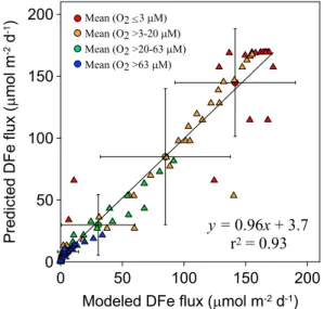
explains 93% of the variance in the modeled rates, with a standard error of the slope of 0.027μmol m2d1 (Figure 4). COX and O2BW alone each explain less than 20%. More complex functions did not improve thefit significantly.
The extreme DFefluxes observed on the Peruvian shelf, Californian Borderland Basins, and the Eel River mouth are not captured by the new function.
One factor to consider may simply be that sediments display a wide range of reactive iron content. In our simulations we used a FeHR/FeT of 0.17, which is within the range of 0.08–0.40 for continental margin sediments [Raiswell and Canfield, 1998]. Rivers tend to deposit large amounts of terrigenous inorganic material on the shelf which may be more enriched in FeHR compared to the global average [Poulton and Raiswell, 2002]. We tested the sensitivity of DFe fluxes to the FeHR content by repeating the model simulations for the shelf site with 1 and 100μM O2BW. In these simulations, the total iron flux was held constant but thefluxes of FeHRand FeUwere varied. The results show a quasi-linear dependence of benthic DFefluxes on the FeHR/FeT ratio with a steeper response when O2BW is in the normal oxic range compared to the anoxic range (Figure 5). The model predicts that the observed variability in FeHR/FeTfor the FeTflux used in the simulations can result in DFefluxes that vary by an order of magnitude. This supports the idea that high DFefluxes on the Eel River shelf are driven by a higher- than-average FeHRcontent [Severmann et al., 2010] and, possibly, seasonal variability too [Severmann et al., 2010;Berelson et al., 2003;Pakhomova et al., 2007]. Similarly, low DFefluxes were calculated from pore water profiles in sediments with a low FeHR content on the South African margin [Homoky et al., 2013]. Clearly, though, the total FeHRflux is the controlling factor on DFe flux rather than FeHR/FeT, the latter of which is likely to be determined by the weathering regime rather than the overallflux of terrigenous material.
By contrast, terrigenous Fe supply to the California Borderland Basins and the shallow Peruvian shelf is very low. Extremely high benthic DFe fluxes in these regions may be caused by the transient occurrence of oxidizing conditions in the bottom water and the focused discharge of DFe after the recurrence of anoxia [Scholz et al., 2011; Noffke et al., 2012]. The idea is that during oxic periods, a thin oxidized layer develops on the sediment surface which favors the precipitation of Fe oxides and mitigates DFe flux to the bottom water. Deposition of particulate Fe oxides from the water column would also be enhanced under these conditions. A resurgence of anoxic conditions favors reductive dissolution of the accumulated oxides, leading to pulsed release of DFe to the bottom water. Moreover, ironfluxes in Figure 5.Sensitivity of modeled benthic DFefluxes in shelf
sediments to the FeHR/FeTratio in particulate iron oxide deposited on the seafloor [Raiswell and Canfield, 1998]. Results are shown for low (1μM) and high (100μM) O2BW. DFefluxes are normalized to the modeled shelffluxes in Figure 1a for O2BW= 1 and 100μM, indicated by the dashed lines.
Figure 4.Comparison of the DFefluxes simulated using the standardized numerical model for each paired O2BW-COX data (black circles in Figure 3) and the DFefluxes predicted using equation (1), color coded according to O2BW(triangles).
The large circles represent the meanflux ± standard deviation in each O2BWinterval. The straight line is the linear regression curve (equation indicated).
such temporally anoxic and occasionally euxinic settings such as the Peruvian shelf may be largely influenced by additional controls such as the availability of sulfide in the pore water and bottom water and benthic boundary layer [Scholz et al., 2014b]. These factors cannot be constrained with our benthic model, as we assume a bottom water sulfide concentration of zero in all model runs. More generally, the magnitude of the terrigenous FeHRflux and/or focused deposition of Fe oxides due to seasonal or other transient effects might play a more important role in generating the observed variability in benthic DFe fluxes than implied by the model.
6. A Revised Estimate for Global Benthic Iron Flux
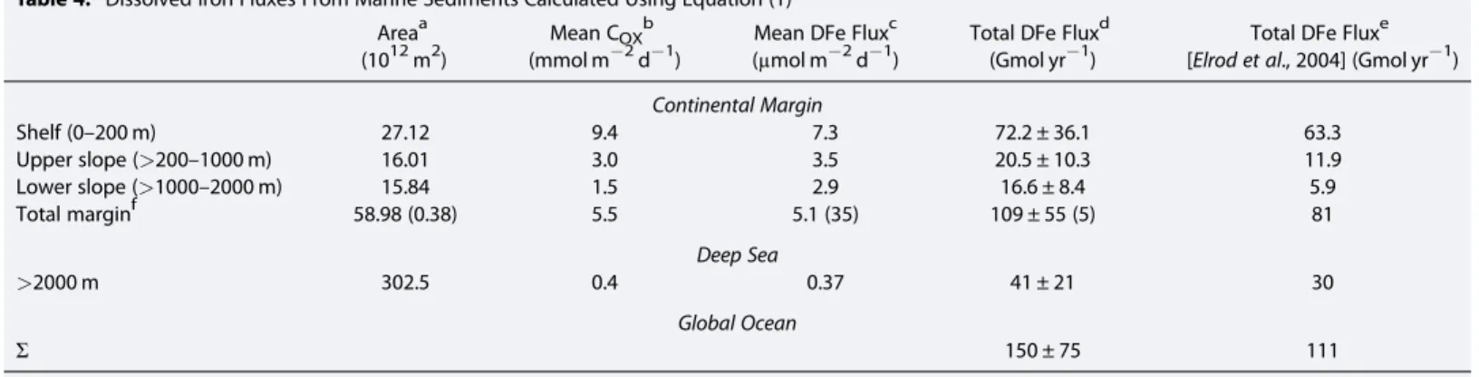
Our new estimate of the global benthic DFeflux is based on spatially resolved bathymetry, O2BW, and COX data. Maps of bathymetry and O2BWon a 1° × 1° resolution were taken fromBohlen et al. [2012] based on data from the World Ocean Atlas [Garcia et al., 2006]. Gridded COXdata are unavailable, and instead, we used average COX for several hypsometric intervals [Burdige, 2007]. Upscaling using the new function (equation (1)) predicts a global DFe flux of 150 ± 75 Gmol yr1 (Table 4), of which 109 ± 55 Gmol yr1 is contributed by continental margin sediments and 41 ± 21 Gmol yr1 by the deep sea (>2000 m). The uncertainties are calculated assuming that variability in FeHR/FeTand FeTcontent contributes to the largest error in the model predictions (see Table 4). This is equivalent to 50% for margin and deep-sea sediments.
However, it is obvious from the scatter in Figure 1 that there are other sources of variability in DFefluxes.
This is not surprising given the physical and biogeochemical heterogeneity of continental margin sediments, implying that the calculated uncertainty is a conservative estimate [Liu et al., 2010].
Note that the average DFeflux from deep-sea sediments is very low (0.37μmol m2d1) yet globally significant by virtue of the vast expanse of the ocean basins. Nonetheless, thisflux is speculative because very few flux measurements have been made in the ocean basins. Sequestration of DFe in deep-sea sediments may be more efficient than predicted, especially if other DFe removal pathways currently ignored in the model are significant, such as precipitation of authigenic carbonates, phosphates, or silicates. Consequently, the data currently only support a global DFeflux of 109 Gmol yr1, but it may be higher, especially if nonreductive iron dissolution contributes significantly to the global Fe budget [Homoky et al., 2013;Conway and John, 2014]. In fact, the Biogeochemical Elemental Cycling ocean model that is tuned to pelagic DFe distribution does consider a very low DFeflux from the lower slope and deep basins [Moore and Braucher, 2008].
Taking the lower global DFeflux of 109 Gmol yr1, our model suggests that two thirds (72 Gmol yr1) is contributed by shelf sediments (Table 4). This is similar to 89 Gmol yr1 derived byElrod et al. [2004]
Table 4. Dissolved Iron Fluxes From Marine Sediments Calculated Using Equation (1) Areaa
(1012m2)
Mean COXb (mmol m2d1)
Mean DFe Fluxc (μmol m2d1)
Total DFe Fluxd (Gmol yr1)
Total DFe Fluxe [Elrod et al., 2004] (Gmol yr1) Continental Margin
Shelf (0–200 m) 27.12 9.4 7.3 72.2 ± 36.1 63.3
Upper slope (>200–1000 m) 16.01 3.0 3.5 20.5 ± 10.3 11.9
Lower slope (>1000–2000 m) 15.84 1.5 2.9 16.6 ± 8.4 5.9
Total marginf 58.98 (0.38) 5.5 5.1 (35) 109 ± 55 (5) 81
Deep Sea
>2000 m 302.5 0.4 0.37 41 ± 21 30
Global Ocean
Σ 150 ± 75 111
aMenard and Smith[1966].
bBurdige[2007].
cUsing the gridded O2BWand bathymetry in combination with equation (1).
dIntegrated over the corresponding ocean area. The uncertainties (±) are calculated based on the uncertainty in FeHRand FeTcontent. Standard deviations in FeHRand FeTare reported for a mean marine sediment byPoulton and Raiswell[2002, Table 7]. Using standard error propagation rules, the relative error in the FeHR/FeTratio using their data is 50%, which is taken as the error in DFeflux.
eTheflux calculated assuming the regression provided byElrod et al. [2004] in Figure 1. For consistency withElrod et al. [2004], we used aflux ratio of 0.68μmol DFe/mmol carbon oxidized in this calculation, ignoring the intercept DFeflux of 0.5μmol m2d1in their linear regression equation.
fValues in parenthesis correspond to sediments underlying oxygen-deficient bottom waters (<20μM).
assuming a mean COXof 12 mmol m2d1. Our lower shelf COX(9.4 mmol m2d1) is derived from a well- constrained empirical relationship between COX and water depth [Burdige, 2007]. Using Burdige’s COX would decrease Elrod et al.’s shelf estimate by around one third. Importantly, however, we find that continental slope sediments are also major sources of iron to ocean bottom waters (37.1 Gmol yr1). The implication is that sedimentary DFe release has been grossly underestimated in the marine Fe budget [Jickells et al., 2005;Boyd and Ellwood, 2010].
Our derived globalflux is 3 to 14 times higher than most previous estimates (see section 1). The average DFeflux from continental margins (5.1μmol m2d1; Table 4) is also 3 to 5 times higher than the maximum benthic DFe flux of 1–2μmol m2d1imposed as a seafloor boundary condition in some global iron models [e.g.,Moore et al., 2004;Aumont and Bopp, 2006]. One reason for the lowerflux estimates from the global approaches may be an underestimation of organic carbon rain rates [Moore and Braucher, 2008]. It would be interesting to compare carbon exportfluxes from these models, but this datum is unfortunately seldom reported. A more important consideration is that carbon rain rates and tracer distributions are generally poorly resolved over shelf sediments in global models, meaning that the shelf DFeflux (72.2 Gmol yr1), equivalent to two thirds of the global sedimentary DFe release, is not properly accounted for. Instead, the models are tuned to the lower DFe fluxes from slope sediments. However, a fraction of the iron released from shelf sediments is not retained in coastal waters but exported offshore in both dissolved and particulate form [Johnson et al., 1999;Lam et al., 2006;Lohan and Bruland, 2008;de Jong et al., 2012]. Too little export of coastal iron to the ocean basins may lead to a too strong dependence of surface iron concentrations on atmospheric iron deposition, thus influencing model sensitivity toward this source [Moore and Braucher, 2008;Tagliabue et al., 2014].
An additional factor to consider that has been highlighted in this study is the role of bottom water oxygen concentration. Comparison of our DFefluxes with those predicted byElrod et al. [2004] using the same COX provides a broad overview of the effect of O2BW. Most notably, wefind that our DFefluxes on the continental slope are 2–3 times higher than predicted by Elrod et al.’s function (Table 4). This is partly because oxygen- deficient waters of the eastern boundary upwelling systems tend to impinge on the seafloor at these depths [Helly and Levin, 2004]. Sediments underlying bottom waters below the 20μM threshold areflux hot spots, releasing DFe at an average rate of 35μmol m2d1. They account for 4% of total DFeflux on the margin despite covering<1% of the seafloor. Yet it should be noted that the relatively coarse 1° × 1° resolution does not accurately capture shallow marginal sediments. Taking a more sophisticated approach,Helly and Levin [2004] estimated that around 1.4 × 10¹²m2of sediments are in contact with bottom water<22μM, which is equivalent to 3% by area of the shelf and upper slope (0–1000 m). Our DFe flux from oxygen-deficient regions is, therefore, likely to be a minimum estimate and may be up to a factor of 3 higher.
7. Impact of Benthic Iron Release on Oceanic Dissolved Iron Distributions
The ability of our simple function to predict DFefluxes is encouraging because it can easily be implemented in global biogeochemical models. Most models routinely simulate dissolved oxygen and organic carbon rain rates to the seafloor (≈COX). Thus, it provides a straightforward tool to test how the spatial distribution of DFe in the ocean is impacted by benthic iron release.
We tested the impact of our predictive function on global iron distributions in the ocean using the University of Victoria Earth System Climate Model (UVic ESCM). This model includes a coupled physical biogeochemical ocean component with a dynamic iron cycle [Nickelsen et al., 2015]. Like other global models, shelf processes are not adequately described due to the coarse spatial resolution. The model has two iron pools, dissolved and particulate, and is similar to other global iron models [e.g.,Moore and Braucher, 2008;Tagliabue et al., 2014]. Scavenging of iron from the water column by organic particles is tuned to provide a good correlation between observed and modeled surface ocean DFe distributions.
The model does not include scavenging by resuspended inorganic particles. Sedimentary iron release is proportional to carbon oxidation rate (i.e., Elrod et al.’s function), and the model further uses a simple oxygen-dependent switch threshold of 5μM. If bottom water O2falls below this value, all iron deposited on the seafloor is released back to the water column. Benthic DFefluxes predicted by the UVic ESCM model are shown in Figure 6a, and tuning of scavenging rates leads to a goodfit to observed surface DFe concentrations (Figure 6b). The global benthic DFeflux predicted by the model in this configuration is 19 Gmol yr1[Nickelsen et al., 2015].