s ) B → µ µ attheLHCwiththeATLAS,CMSandLHCbexperiments 0( + − Searchfortheraredecays

A TLAS-CONF-2012-061 18 June 2012

EUROPEAN ORGANIZATION FOR NUCLEAR RESEARCH (CERN)

LHCb-CONF-2012-017 CMS-PAS-BPH-12-009 ATLAS-CONF-2012-061 June 18, 2012

Search for the rare decays B ⁰

(s) → µ ⁺ µ ⁻ at the LHC

with the ATLAS, CMS and LHCb experiments

The ATLAS, CMS, and LHCb collaborations

Abstract

A combination of the results of the search for the decay B

→ µ

µ

is performed using about 2.4 fb

, 5 fb

and 1.0 fb

of pp collisions at √

s = 7 TeV, collected at the Large Hadron Collider at CERN by the ATLAS, CMS, and LHCb experiments, respectively. The observed candidates in the three experiments are consistent with the expectation from the sum of background and Standard Model signal processes within 1σ. The combination results in upper limits on the branching fractions, B(B

→ µ

µ

)

< 4.2 × 10

and B(B

→ µ

µ

) < 8.1 × 10

both at 95% confidence level.

1

Conference report prepared for the Physics at Large Hadron Collider conference, Vancouver, 4-9 June

2012.

1 Introduction

Within the Standard Model (SM) the exclusive dimuon decays of B

and B

mesons are rare, as they occur only via helicity suppressed loop diagrams. The predicted branching fractions used in this combination are those provided in [1] :

B(B

→ µ

µ

)

= (3.2 ± 0.2) × 10

B(B

→ µ

µ

)

= (1.0 ± 0.1) × 10

.

As described in [2], the experimentally measured observable for B

→ µ

µ

is the time integrated branching fraction. The previous theoretical prediction should be enlarged by 9% to take into account the time evolution of the initial state. In this note, no correction has been applied.

Theories beyond the SM (referred to as new physics, or NP), especially those with an extended Higgs sector, can significantly enhance these branching fractions. This is particularly true for Supersymmetric (SUSY) models in which the contributions at high tan β can be quite large [3], even after applying other experimental constraints [4, 5].

In fact, constrained fits to SUSY models with few free parameters, such as CMSSM and NUHM1, are predictive enough to provide expectations for B(B

→ µ

µ

) [4]:

B(B

→ µ

µ

)

B(B

→ µ

µ

)

≈ 1.2

B(B

→ µ

µ

)

B(B

→ µ

µ

)

≈ 1.9

.

The most restrictive limits on the search for B

→ µ

µ

and B

→ µ

µ

have so far been achieved by LHCb with 1.0 fb

of integrated luminosity of pp collisions at √

s = 7 TeV collected in 2011 [6]:

B(B

→ µ

µ

) < 4.5 × 10

at 95% Confidence Level (C.L.) B(B

→ µ

µ

) < 10 × 10

at 95% C.L.

For B

→ µ

µ

the observed data show a slight excess over the background-only hypoth- esis (p-value of 18%), which is consistent with the presence of a SM signal.

The LHCb collaboration had also analyzed independently 0.037 fb

of integrated luminosity of pp collisions at √

s = 7 TeV collected in 2010 [7]. This analysis provides upper limits of B(B

→ µ

µ

) < 56 × 10

and B(B

→ µ

µ

) < 150 × 10

at 95%

C.L.

The ATLAS collaboration has analyzed a total of 2.4 fb

of pp collisions at √ s = 7 TeV [8]. No excess of events over the background expectation is found, giving an upper limit of B(B

→ µ

µ

) < 22 × 10

at 95% C.L.

The CMS collaboration has analyzed a total of 5 fb

of pp collisions at √

s = 7 TeV

collected in 2011 [9]. The number of events observed is consistent with the expectation

from background plus SM signal predictions. The resulting upper limits on the branching fractions are B(B

→ µ

µ

) < 7.7 × 10

and B(B

→ µ

µ

) < 1.8 × 10

at 95%

C.L. These results were calculated using the profile likelihood test statistic with profiled nuisance parameters (including B

and B

crossfeed) and a sideband window sampling which is a very conservative approach. In the combination performed in this note, a second approach was used, as described in Sect. 2. This approach gives upper limits of B(B

→ µ

µ

) < 7.2 × 10

and B(B

→ µ

µ

) < 1.6 × 10

at 95% C.L. for CMS.

For ATLAS and CMS the expected number of signal events is evaluated using a nor- malization factor computed from the observed number of B

→ J/ψK

events using the value of f

/f

from LHCb [10], f

/f

= 0.267± 0.021. This value is assumed to be valid for the pseudorapidity range of ATLAS and CMS and no additional systematic uncertainty with respect to f

/f

is assigned. For LHCb, the expected number of signal events is computed using a combination of three normalization factors obtained from the numbers of B

→ J/ψK

, B

→ J/ψφ and B

→ K

π

candidates.

In this note, the ATLAS, CMS and LHCb results on the search for B

→ µ

µ

decays and the CMS and LHCb ones on the search for B

→ µ

µ

are combined. The combination uses the modified frequentist approach, or CL

method [11]. While ATLAS and CMS benefit from a larger integrated luminosity, LHCb benefits from the large b ¯ b production cross-section at large pseudorapidity and the capability to reconstruct and trigger on low transverse momentum muons. The results of the CDF [12] and D0 [13]

collaborations are not included in the combination.

2 Input to the combination

2.1 ATLAS analysis

The ATLAS B

→ µ

µ

search, based on the first 2.4 fb

of 2011 data [8], is performed in three bins of |η|

, the maximum pseudorapidity (|η|) value of the two decay muons.

The likelihood used in the limit extraction with the CL

method by ATLAS is given by:

L = G(

|, σ

) G(R

|R

, σ

) · (1)

Nbins

Y

i=1

P (N

|

BR + N

+ N

) P (N

|R

R

N

) G(

|

, σ

)

with N

= 3, P (...) denoting the signal and background Poisson distributions and

G(...) the Gaussian distributions modelling the uncertainties of the nuisance parameters,

i.e. of the global efficiency , of the background-to-signal-region ratio R and an additional

Gaussian term describing the uncorrelated part of the errors on the relative efficiencies

. N

indicates the number of combinatorial background events, while N

indicates

the number of peaking background events coming from misreconstructed B

→ h

h

events. The inverse of the product of the global () and relative (

) efficiencies

is the single-event-sensitivity (SES) per bin, i.e. SES = (

)

.

Table 1 provides the ATLAS input values used in the CL

extraction. It is important to note that the signal extraction is optimized using half of the background sample in the sidebands (events with odd event numbers) while the other half (events with even event numbers) is used to estimate the combinatorial background in the signal region from the sidebands. This avoids an optimization bias of about 30% on the upper limit as described in more detail in Section 6 of [8], while it effectively reduces the size of the data sample available for the background determination from the sidebands by a factor of two.

No ATLAS data is used in the determination of the B(B

→ µ

µ

) combined limit.

Table 1: Input values used for the extraction of the B

→ µ

µ

upper limit using the CL

method from the ATLAS analysis of the first 2.4 fb

of the 2011 data [8]. The values are given for three bins in |η|

, the maximum |η| value of the two signal decay muons:

barrel (|η|

< 1.0), transition (1.0 < |η|

< 1.5) and endcap (1.5 < |η|

< 2.5) region. The signal region is defined to be the mass ranges 5250 – 5482, 5234 – 5498 and 5195 – 5537 MeV/c

for the three bins, respectively. The quoted uncertainties include both statistical and systematic sources, combined in quadrature. Parameters indicated as constants (const.) have no errors, either (R

) because the uncertainty is common to the three bins and included in the corresponding global term, or (N

0

(s)→h⁺h⁻

i

) because

the uncertainty does not affect the final result.

Region Barrel Transition Endcap

Global efficiency (4.45 ± 0.45) · 10

Global bkg. scaling factor R

1.00 ± 0.04

Relative efficiencies

[10

] 3.14 ± 0.17 1.40 ± 0.15 1.58 ± 0.26 Relative bkg. scaling factors R

(const.) 1.29 1.14 0.88

Observed in signal region N

2 1 0

Observed in sideband regions N

5 0 2

Exp. peaking bkg. in sig. region N

(const.) 0.10 0.06 0.08

2.2 CMS analysis

Since the background level depends significantly on the pseudorapidity of the B candidate, the CMS analysis is performed separately in two channels, “barrel” and “endcap”, and then combined for the final result [9]. The barrel channel contains the candidates where both muons have |η| < 1.4 and the endcap channel contains those where at least one muon

2

These efficiencies include signal detection efficiencies as well as normalization channel yields and

cross-sections.

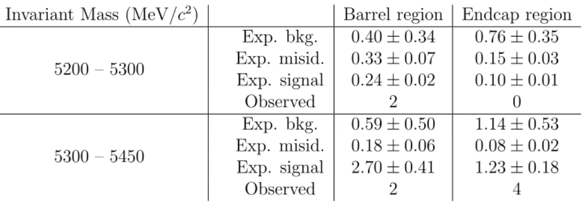
Table 2: Expected background events (excluding misidentification), expected background events from misidentification, expected signal events assuming the SM branching fraction prediction, and observed events in the B

→ µ

µ

and B

→ µ

µ

search windows, from the CMS analysis of the 2011 data. The mass range 5200 – 5300 MeV/c

is associated with the B

window and 5300 – 5450 MeV/c

with the B

window. Uncertainties include systematic effects.

Invariant Mass (MeV/c

) Barrel region Endcap region 5200 – 5300

Exp. bkg. 0.40 ± 0.34 0.76 ± 0.35 Exp. misid. 0.33 ± 0.07 0.15 ± 0.03 Exp. signal 0.24 ± 0.02 0.10 ± 0.01

Observed 2 0

5300 – 5450

Exp. bkg. 0.59 ± 0.50 1.14 ± 0.53 Exp. misid. 0.18 ± 0.06 0.08 ± 0.02 Exp. signal 2.70 ± 0.41 1.23 ± 0.18

Observed 2 4

has |η| > 1.4. The expected number of combinatorial background events in the search window quoted in the table is extracted from a fit to the invariant mass sidebands. The contribution of the misidentified peaking background from B

→ h

h

in the B

search window is very small, as can be seen in Table 2. The only relevant correlation between uncertainties is due to the uncertainty on f

/f

, which is assumed 100% correlated between the number of expected signal events in the barrel and endcap regions. Other sources of correlation, such as the uncertainty on B(B

→ J/ψK

), are negligible at the current level of precision.

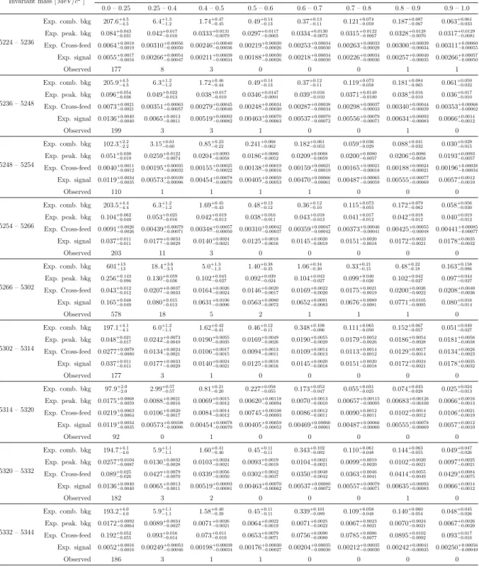
2.3 LHCb analyses

The two LHCb analyses [6, 7] are performed in the LHCb pseudorapidity coverage (2 <

|η| < 6) and are very similar. They proceed by classifying the observed events in bins

of a two dimensional space made of a multivariate discriminant variable and the dimuon

invariant mass. The probability of a signal event to fall in each bin is obtained from

the data sample itself using B

→ h

h

decays to evaluate the distribution of the

multivariate discriminant and dimuon resonances to measure the dimuon invariant mass

resolution. The expected number of combinatorial background events is extracted from a

fit to the invariant mass sidebands. The misidentified peaking background was negligible

in the 2010 analysis. In the 2011 analysis its distribution was derived by applying the

probability for hadrons to be misidentified, obtained from D → K

π

data in bins of

momentum and transverse momentum, to the spectrum of a selected simulated B

→

h

h

sample. While only 0.5

misidentified B

→ h

h

are expected in the B

mass

window, a larger contribution, 2.6

, is expected in the B

mass window. Tables 5, 6

and Tables 7, 8 show, for the 2010 and 2011 analyses, the expected yields of signal and

background events in the B

and B

mass windows in bins of the two dimensional space.

The main systematic uncertainty on the signal yields stems from f

/f

. This parameter is taken 100% correlated between all the bins and all four analyses. Table 5 and Table 6 have therefore been updated from [7] to include the latest f

/f

value [10] used by the three other analyses.

3 Combination procedure

The observed data pattern is subjected to a likelihood ratio test of two hypotheses. In the background scenario it is assumed that the data receive contributions from background processes only, while in the signal-plus-background scenario the contributions from a given value of B(B

→ µ

µ

) are assumed in addition.

In a search experiment, the likelihood ratio Q = L

/L

= Y

i

e

(s

+ b

)

/d

!

e

(b

)

/d

! (2) makes efficient use of the information contained in the event configuration. The likeli- hood ratio in each bin i depends on the expected number of signal events, s

, the expected number of background events, b

and the observed number of events, d

. For convenience, the logarithmic form −2 ln Q is used as the test statistic since this quantity is approx- imately equal to the difference in χ

when the data configuration is compared to the background-only and signal-plus-background hypotheses.

The CL

(CL

) is defined as the probability for signal plus background (background only) to have a value of −2 ln Q less than or equal to that observed in the data. The

−2 ln Q distribution expected for the signal plus background (background only) hypoth- esis is sampled by computing the test statistic from (2) with d

generated according to the signal plus background (background only) expectation. The CL

(CL

) are then derived by computing the fraction of signal plus background (background only) pseudo- experiments with a value of −2 ln Q smaller than or equal to the observed value. Sys- tematic uncertainties are incorporated during the generation of the pseudoexperiments by randomly varying the nuisance parameters, using Poisson distributions for the nuisance parameters which have statistical nature (such as number of events in the sidebands) and bifurcated Gaussians for the others. For a given source of uncertainty, correlations are addressed by applying these random variations simultaneously to all those bins where the uncertainty is relevant. All bins presented in Tables 1, 2 and 5–8 are used in the combination. For the B

→ µ

µ

result 3 ATLAS and 2 CMS bins are combined with the 24 (72) LHCb bins from the 2010 (2011) analysis.

The CL

is the ratio of confidence levels

b

used to set the exclusion (upper) limit

on the branching fraction of the two decays, whereas 1 − CL

is used as a p-value to claim

evidence or observation. A 95(90)% confidence level exclusion corresponds to CL

=

0.05(0.1). A 3σ evidence corresponds to 1 − CL

= 2.7 × 10

and a 5σ discovery to

1 − CL

= 5.73 × 10

for one–sided definition of the significance (for two–sided definition these numbers are 1 − CL

= 1.35 × 10

and 1 − CL

= 2.87 × 10

, respectively).

The use of CL

instead of CL

is chosen to protect against negative statistical fluc- tuations of the background, which could potentially lead to the exclusion of the null hypothesis, even without any experimental sensitivity.

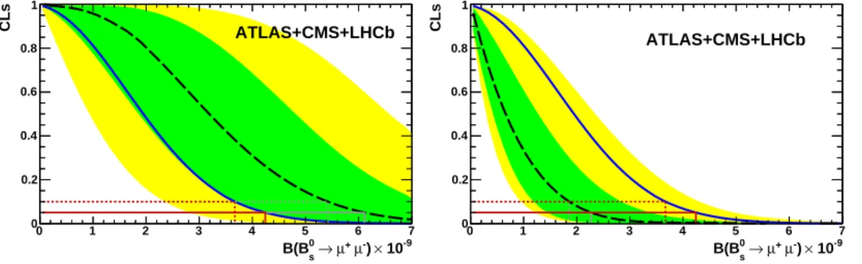
4 Results and conclusions

The expected and observed CL

values derived from ATLAS, CMS, and the two LHCb analyses are shown in Figure 1 as a function of the assumed B(B

→ µ

µ

). The expected and measured limits are reported in the first row of Table 3. This observed distribution of events, when compared with the expected background distribution, results in 1 − CL

(or p-value) of 5%,

and in 1 − CL

of 84% when compared with the expected background plus SM signal distribution, indicating a slight excess of events with respect to the background predictions, compatible with a SM signal within one standard deviation.

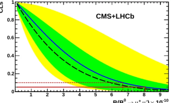
The expected and observed CL

value derived from CMS and the two LHCb analyses are shown in Figure 2 as a function of the assumed B(B

→ µ

µ

). The expected and measured limits are reported in the second row of Table 3.

Table 3: Expected and observed upper limit on B(B

→ µ

µ

), obtained from the combination of ATLAS, CMS, and the two LHCb analyses for B

→ µ

µ

and from CMS and the two LHCb analyses for B

→ µ

µ

. The expected limits correspond to the median cases in which only bkg or SM+bkg events were observed.

bkg only SM + bkg Observed C.L. 90% 95% 90% 95% 90% 95%

B(B

→ µ

µ

) (10

) 1.9 2.3 5.4 6.1 3.7 4.2 B(B

→ µ

µ

) (10

) 5.9 7.3 6.7 8.1

The combined upper limits on B(B

→ µ

µ

) and B(B

→ µ

µ

) improve on the limits obtained by the individual experiments as shown in Table 4, and represent the best existing limits on these decays. The expected limit, if background plus B

→ µ

µ

signal events were observed at the SM rate, improves by 15% with respect to the 2011 LHCb analysis. The improvement on the expected limit in absence of a B

→ µ

µ

signal is 32%.

The observed data is compatible with the SM signal prediction within 1 sigma and NP enhancements of B(B

→ µ

µ

) are constrained to be much smaller than the SM prediction. There remains, however, room for a contribution from physics beyond the SM, including destructive interference between NP and SM which could still cause B(B

→

3

CL

is evaluated at the value of B(B

→ µ

µ

) in which CL

=0.5.

Table 4: Expected and observed upper limit at 95% C.L. on B(B

→ µ

µ

), published by the each experiment and their combination. The expected limits correspond to the median cases in which only bkg or SM+bkg events were observed. For CMS, the numbers in parentheses correspond to the analysis used in the combination.

Mode Limit ATLAS CMS LHCb LHCb

Combined 2010 2011

B

→ µ

µ

(10

)

Bkg Only 23 (3.6) 65 3.4 2.3

Bkg+SM 8.4 7.2 6.1

Obs 22 7.7 (7.2) 56 4.5 4.2

B

→ µ

µ

(10

)

Bkg Only – (13) 180 11 7.3

Bkg+SM – 16

Obs – 14 (16) 150 10 8.1

µ

µ

) to be significantly smaller than the SM prediction. Such cases can be probed by the LHC experiments with more integrated luminosity.

10-9

×

-) µ µ+ s→ B(B0

0 1 2 3 4 5 6 7

CLs

0 0.2 0.4 0.6 0.8 1

ATLAS+CMS+LHCb

10-9

×

-) µ µ+ s→ B(B0

0 1 2 3 4 5 6 7

CLs

0 0.2 0.4 0.6 0.8 1

ATLAS+CMS+LHCb

Figure 1: CL

as a function of the assumed branching fraction for B

→ µ

µ

. The

dashed black curves are the medians of the expected CL

distributions, if background and

SM signal were observed (left), and in complete absence of signal (right). The green (yel-

low) areas cover, for each branching fraction, 34% (48%) of the expected CL

distribution

on each side of its median, corresponding to ±1(2)σ intervals. The solid blue curves are

the observed CL

. The upper limits at 90 % (95 %) C.L. are indicated by the dotted (solid)

horizontal lines in red (dark gray) for the observation and in gray for the expectation.

0 0.1 0.2 0.3 0.4 0.5 0.6 0.7 0.8 0.9

CLs

0 0.2 0.4 0.6 0.8 1

10-10

×

-) µ µ+

→ B(B0

1 2 3 4 5 6 7 8 9

CMS+LHCb

Figure 2: CL

as a function of the assumed branching fraction for B

→ µ

µ

. The dashed black curve is the median of the expected CL

distributions in absence of signal.

The green (yellow) area covers, for each branching fraction, 34% (48%) of the expected

CL

distribution on each side of its median, corresponding to ±1(2)σ intervals. The solid

blue curve is the observed CL

. The upper limits at 90 % (95 %) C.L. are indicated by

the dotted (solid) horizontal lines in red (dark gray) for the observation and in gray for

the expectation.

References

[1] A. J. Buras, M. V. Carlucci, S. Gori, and G. Isidori, Higgs-mediated FCNCs: nat- ural flavour conservation vs. minimal flavour violation, JHEP 1010 (2010) 009, arXiv:1005.5310; A. J. Buras, Minimal flavour violation and beyond: towards a flavour code for short distance dynamics, Acta Phys. Polon. B41 (2010) 2487, arXiv:1012.1447.

[2] K. de Bruyn et al., A New Window for New Physics in B

→ µ

µ

, arXiv:1204.1737.

[3] S. Choudhury and N. Gaur, Dileptonic decay of B

meson in SUSY models with large tanβ, Phys. Lett. B451 (1999) 86; C. Hamzaoui, M. Pospelov, and M. Toharia, Higgs mediated FCNC in supersymmetric models with large tan β, Phys. Rev. D59 (1999) 095005; K. Babu and C. F. Kolda, Higgs mediated B

→ µ

µ

in minimal supersymmetry, Phys. Rev. Lett. 84 (2000) 228; L. J. Hall, R. Rattazzi, and U. Sarid, The top quark mass in supersymmetric SO(10) unification, Phys. Rev. D50 (1994) 7048; C.-S. Huang, W. Liao, and Q.-S. Yan, The promising process to distinguish supersymmetric models with large tan β from the standard model: B → X(s)µ

µ

, Phys. Rev. D59 (1999) 011701.

[4] O. Buchmueller et al., Higgs and Supersymmetry, arXiv:1112.3564, to appear in Eur. J. Phys C.

[5] D. Feldman, K. Freese, P. Nath, B. D. Nelson, and G. Peim, Predictive Signatures of Supersymmetry: Measuring the Dark Matter Mass and Gluino Mass with Early LHC data, Phys. Rev. D84 (2011) 015007, arXiv:1102.2548; S. Scopel, S. Choi, N. Fornengo, and A. Bottino, Impact of the recent results by the CMS and AT- LAS Collaborations at the CERN Large Hadron Collider on an effective Minimal Supersymmetric extension of the Standard Model, Phys. Rev. D83 (2011) 095016, arXiv:1102.4033; P. Bechtle et al., What if the LHC does not find supersymme- try in the sqrt(s)=7 TeV run?, Phys. Rev. D84 (2011) 011701, arXiv:1102.4693;

S. Akula et al., Interpreting the First CMS and ATLAS SUSY Results, Phys. Lett.

B699 (2011) 377, arXiv:1103.1197; S. Akula, D. Feldman, Z. Liu, P. Nath, and G. Peim, New Constraints on Dark Matter from CMS and ATLAS Data, Mod.

Phys. Lett. A26 (2011) 1521, arXiv:1103.5061; M. Farina et al., Implications of XENON100 and LHC results for Dark Matter models, Nucl. Phys. B853 (2011) 607, arXiv:1104.3572; S. Profumo, The Quest for Supersymmetry: Early LHC Results versus Direct and Indirect Neutralino Dark Matter Searches, Phys. Rev. D84 (2011) 015008, arXiv:1105.5162; T. Li, J. A. Maxin, D. V. Nanopoulos, and J. W. Walker, The Race for Supersymmetric Dark Matter at XENON100 and the LHC: Stringy Correlations from No-Scale F-SU(5), arXiv:1106.1165.

[6] LHCb collaboration, R. Aaij et al., Strong constraints on the rare decays B

→ µ

µ

and B

→ µ

µ

, Phys. Rev. Lett. 108 (2012) 231801, arXiv:1203.4493.

[7] LHCb Collaboration, R. Aaij et al., Search for the rare decays B

→ µµ and B

→ µµ, Phys. Lett. B699 (2011) 330, arXiv:1103.2465.

[8] ATLAS Collaboration, G. Aad et al., Search for the decay B

→ µ

µ

with the ATLAS detector, arXiv:1204.0735.

[9] CMS Collaboration, S. Chatrchyan et al., Search for B

→ µ

µ

and B

→ µ

µ

decays, JHEP 1204 (2012) 033, arXiv:1203.3976.

[10] LHCb collaboration, R. Aaij et al., Measurement of b hadron production fractions in 7 TeV pp collisions, Phys. Rev. D85 (2012) 032008, arXiv:1111.2357.

[11] T. Junk, Confidence level computation for combining searches with small statistics, Nucl. Instrum. Meth. A434 (1999) 435, arXiv:hep-ex/9902006; A. Read, Presen- tation of search results: the CL

technique, J. Phys. G28 (2002) 2693.

[12] CDF collaboration, T. Aaltonen et al., Search for B

→ µ

µ

and B

→ µ

µ

decays with CDF II, Phys. Rev. Lett. 107 (2011) 191801, arXiv:1107.2304.

[13] DØ collaboration, V. M. Abazov et al., Search for the rare decay B

→ µ

µ

, Phys.

Lett. B693 (2010) 539, arXiv:1006.3469.

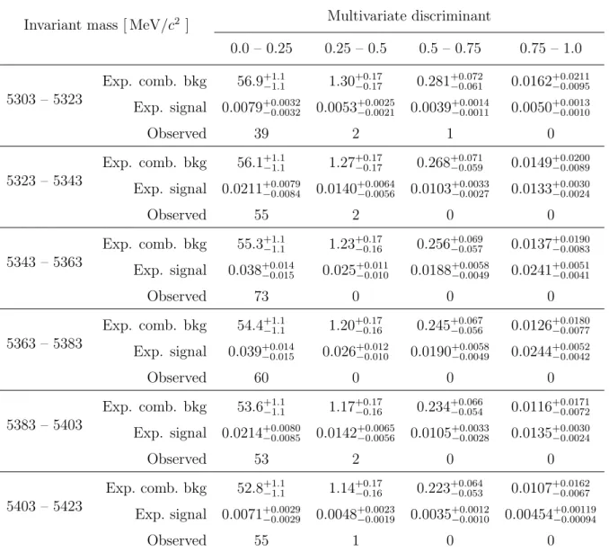
Table 5: Expected background events, expected signal events assuming the SM branching ratio prediction, and observed events in bins of invariant mass and multivariate discriminant in the B

→ µ

µ

search window, from the LHCb analysis of the 2010 data.

Invariant mass [ MeV/c

] Multivariate discriminant

0.0 – 0.25 0.25 – 0.5 0.5 – 0.75 0.75 – 1.0

5303 – 5323

Exp. comb. bkg 56.9

1.30

0.281

0.0162

Exp. signal 0.0079

0.0053

0.0039

0.0050

Observed 39 2 1 0

5323 – 5343

Exp. comb. bkg 56.1

1.27

0.268

0.0149

Exp. signal 0.0211

0.0140

0.0103

0.0133

Observed 55 2 0 0

5343 – 5363

Exp. comb. bkg 55.3

1.23

0.256

0.0137

Exp. signal 0.038

0.025

0.0188

0.0241

Observed 73 0 0 0

5363 – 5383

Exp. comb. bkg 54.4

1.20

0.245

0.0126

Exp. signal 0.039

0.026

0.0190

0.0244

Observed 60 0 0 0

5383 – 5403

Exp. comb. bkg 53.6

1.17

0.234

0.0116

Exp. signal 0.0214

0.0142

0.0105

0.0135

Observed 53 2 0 0

5403 – 5423

Exp. comb. bkg 52.8

1.14

0.223

0.0107

Exp. signal 0.0071

0.0048

0.0035

0.00454

Observed 55 1 0 0

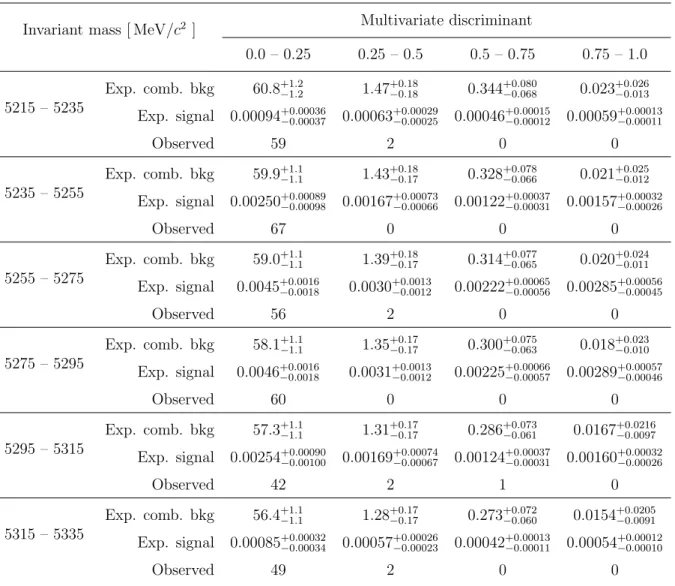
Table 6: Expected background, expected SM signal and observed number of events in bins of invariant mass and multivariate discriminant in the B

→ µ

µ

search window, from the LHCb analysis of the 2010 data.

Invariant mass [ MeV/c

] Multivariate discriminant

0.0 – 0.25 0.25 – 0.5 0.5 – 0.75 0.75 – 1.0

5215 – 5235

Exp. comb. bkg 60.8

1.47

0.344

0.023

Exp. signal 0.00094

0.00063

0.00046

0.00059

Observed 59 2 0 0

5235 – 5255

Exp. comb. bkg 59.9

1.43

0.328

0.021

Exp. signal 0.00250

0.00167

0.00122

0.00157

Observed 67 0 0 0

5255 – 5275

Exp. comb. bkg 59.0

1.39

0.314

0.020

Exp. signal 0.0045

0.0030

0.00222

0.00285

Observed 56 2 0 0

5275 – 5295

Exp. comb. bkg 58.1

1.35

0.300

0.018

Exp. signal 0.0046

0.0031

0.00225

0.00289

Observed 60 0 0 0

5295 – 5315

Exp. comb. bkg 57.3

1.31

0.286

0.0167

Exp. signal 0.00254

0.00169

0.00124

0.00160

Observed 42 2 1 0

5315 – 5335

Exp. comb. bkg 56.4

1.28

0.273

0.0154

Exp. signal 0.00085

0.00057

0.00042

0.00054

Observed 49 2 0 0

Table 7: B

→ µ

µ

: Expected combinatorial background events, expected peaking (B

→ h

h

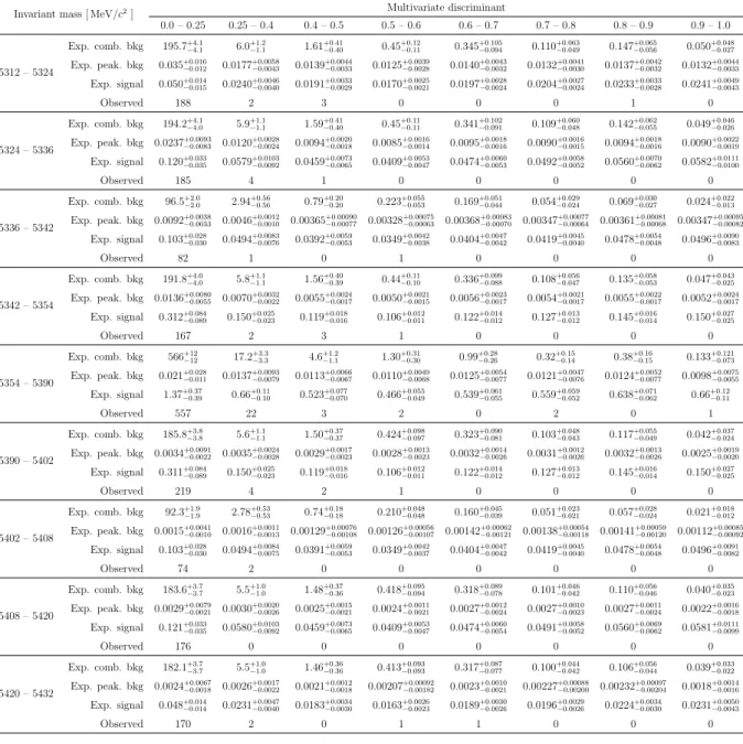
) background events and, expected signal events assuming the SM branching fraction prediction in bins of invariant mass and multivariate discriminant , from the LHCb analysis of the 2011 data.

Invariant mass [ MeV/c²] Multivariate discriminant

0.0 – 0.25 0.25 – 0.4 0.4 – 0.5 0.5 – 0.6 0.6 – 0.7 0.7 – 0.8 0.8 – 0.9 0.9 – 1.0

5312 – 5324

Exp. comb. bkg 195.7^+4.1_−4.1 6.0^+1.2_−1.1 1.61^+0.41_−0.40 0.45^+0.12_−0.11 0.345^+0.105_−0.094 0.110^+0.063_−0.049 0.147^+0.065_−0.056 0.050^+0.048_−0.027 Exp. peak. bkg 0.035^+0.016−0.012 0.0177^+0.0058−0.0043 0.0139^+0.0044−0.0033 0.0125^+0.0039−0.0028 0.0140^+0.0043−0.0032 0.0132^+0.0041−0.0030 0.0137^+0.0042−0.0032 0.0132^+0.0044−0.0033

Exp. signal 0.050^+0.014−0.015 0.0240^+0.0046−0.0040 0.0191^+0.0033−0.0029 0.0170^+0.0025−0.0021 0.0197^+0.0028−0.0024 0.0204^+0.0027−0.0024 0.0233^+0.0033−0.0028 0.0241^+0.0049−0.0043

Observed 188 2 3 0 0 0 1 0

5324 – 5336

Exp. comb. bkg 194.2^+4.1−4.0 5.9^+1.1−1.1 1.59^+0.41−0.40 0.45^+0.11−0.11 0.341^+0.102−0.091 0.109^+0.060−0.048 0.142^+0.062−0.055 0.049^+0.046−0.026

Exp. peak. bkg 0.0237^+0.0093−0.0083 0.0120^+0.0028−0.0024 0.0094^+0.0020−0.0018 0.0085^+0.0016−0.0014 0.0095^+0.0018−0.0016 0.0090^+0.0016−0.0015 0.0094^+0.0018−0.0016 0.0090^+0.0022−0.0019

Exp. signal 0.120^+0.033_−0.035 0.0579^+0.0103_−0.0092 0.0459^+0.0073_−0.0065 0.0409^+0.0053_−0.0047 0.0474^+0.0060_−0.0053 0.0492^+0.0058_−0.0052 0.0560^+0.0070_−0.0062 0.0582^+0.0111_−0.0100

Observed 185 4 1 0 0 0 0 0

5336 – 5342

Exp. comb. bkg 96.5^+2.0_−2.0 2.94^+0.56_−0.56 0.79^+0.20_−0.20 0.223^+0.055_−0.053 0.169^+0.051_−0.044 0.054^+0.029_−0.024 0.069^+0.030_−0.027 0.024^+0.022_−0.013 Exp. peak. bkg 0.0092^+0.0038−0.0033 0.0046^+0.0012−0.0010 0.00365^+0.00090−0.00077 0.00328^+0.00075−0.00063 0.00368^+0.00083−0.00070 0.00347^+0.00077−0.00064 0.00361^+0.00081−0.00068 0.00347^+0.00095−0.00082

Exp. signal 0.103^+0.028−0.030 0.0494^+0.0083−0.0076 0.0392^+0.0059−0.0053 0.0349^+0.0042−0.0038 0.0404^+0.0047−0.0042 0.0419^+0.0045−0.0040 0.0478^+0.0054−0.0048 0.0496^+0.0090−0.0083

Observed 82 1 0 1 0 0 0 0

5342 – 5354

Exp. comb. bkg 191.8^+4.0−4.0 5.8^+1.1−1.1 1.56^+0.40−0.39 0.44^+0.11−0.10 0.336^+0.099−0.088 0.108^+0.056−0.047 0.135^+0.058−0.053 0.047^+0.043−0.025

Exp. peak. bkg 0.0136^+0.0080−0.0055 0.0070^+0.0032−0.0022 0.0055^+0.0024−0.0017 0.0050^+0.0021−0.0015 0.0056^+0.0023−0.0017 0.0054^+0.0021−0.0017 0.0055^+0.0022−0.0017 0.0052^+0.0024−0.0017

Exp. signal 0.312^+0.084_−0.089 0.150^+0.025_−0.023 0.119^+0.018_−0.016 0.106^+0.012_−0.011 0.122^+0.014_−0.012 0.127^+0.013_−0.012 0.145^+0.016_−0.014 0.150^+0.027_−0.025

Observed 167 2 3 1 0 0 0 0

5354 – 5390

Exp. comb. bkg 566⁺¹²₋₁₂ 17.2^+3.3_−3.3 4.6^+1.2_−1.1 1.30^+0.31_−0.30 0.99^+0.28_−0.26 0.32^+0.15_−0.14 0.38^+0.16_−0.15 0.133^+0.121_−0.073 Exp. peak. bkg 0.021^+0.028−0.011 0.0137^+0.0093−0.0079 0.0113^+0.0066−0.0067 0.0110^+0.0049−0.0068 0.0125^+0.0054−0.0077 0.0121^+0.0047−0.0076 0.0124^+0.0052−0.0077 0.0098^+0.0075−0.0055

Exp. signal 1.37^+0.37−0.39 0.66^+0.11−0.10 0.523^+0.077−0.070 0.466^+0.055−0.049 0.539^+0.061−0.055 0.559^+0.059−0.052 0.638^+0.071−0.062 0.66^+0.12−0.11

Observed 557 22 3 2 0 2 0 1

5390 – 5402

Exp. comb. bkg 185.8^+3.8−3.8 5.6^+1.1−1.1 1.50^+0.37−0.37 0.424^+0.098−0.097 0.323^+0.090−0.081 0.103^+0.048−0.043 0.117^+0.055−0.049 0.042^+0.037−0.024

Exp. peak. bkg 0.0034^+0.0091−0.0022 0.0035^+0.0024−0.0028 0.0029^+0.0017−0.0023 0.0028^+0.0013−0.0023 0.0032^+0.0014−0.0026 0.0031^+0.0012−0.0026 0.0032^+0.0013−0.0026 0.0025^+0.0019−0.0020

Exp. signal 0.311^+0.084_−0.089 0.150^+0.025_−0.023 0.119^+0.018_−0.016 0.106^+0.012_−0.011 0.122^+0.014_−0.012 0.127^+0.013_−0.012 0.145^+0.016_−0.014 0.150^+0.027_−0.025

Observed 219 4 2 1 0 0 0 0

5402 – 5408

Exp. comb. bkg 92.3^+1.9_−1.9 2.78^+0.53_−0.53 0.74^+0.18_−0.18 0.210^+0.048_−0.048 0.160^+0.045_−0.039 0.051^+0.023_−0.021 0.057^+0.028_−0.024 0.021^+0.018_−0.012 Exp. peak. bkg 0.0015^+0.0041−0.0010 0.0016^+0.0011−0.0013 0.00129^+0.00076−0.00108 0.00126^+0.00056−0.00107 0.00142^+0.00062−0.00121 0.00138^+0.00054−0.00118 0.00141^+0.00059−0.00120 0.00112^+0.00085−0.00092

Exp. signal 0.103^+0.028−0.030 0.0494^+0.0084−0.0075 0.0391^+0.0059−0.0053 0.0349^+0.0042−0.0037 0.0404^+0.0047−0.0042 0.0419^+0.0045−0.0040 0.0478^+0.0054−0.0048 0.0496^+0.0091−0.0082

Observed 74 2 0 0 0 0 0 0

5408 – 5420

Exp. comb. bkg 183.6^+3.7−3.7 5.5^+1.0−1.0 1.48^+0.37−0.36 0.418^+0.095−0.094 0.318^+0.089−0.078 0.101^+0.046−0.042 0.110^+0.056−0.046 0.040^+0.035−0.023

Exp. peak. bkg 0.0029^+0.0079−0.0021 0.0030^+0.0020−0.0026 0.0025^+0.0015−0.0021 0.0024^+0.0011−0.0021 0.0027^+0.0012−0.0024 0.0027^+0.0010−0.0023 0.0027^+0.0011−0.0024 0.0022^+0.0016−0.0018

Exp. signal 0.121^+0.033_−0.035 0.0580^+0.0103_−0.0092 0.0459^+0.0073_−0.0065 0.0409^+0.0053_−0.0047 0.0474^+0.0060_−0.0054 0.0491^+0.0058_−0.0052 0.0560^+0.0069_−0.0062 0.0581^+0.0111_−0.0099

Observed 176 0 0 0 0 0 0 0

5420 – 5432

Exp. comb. bkg 182.1^+3.7−3.7 5.5^+1.0−1.0 1.46^+0.36−0.36 0.413^+0.093−0.093 0.317^+0.087−0.077 0.100^+0.044−0.042 0.106^+0.056−0.044 0.039^+0.033−0.022

Exp. peak. bkg 0.0024^+0.0067−0.0018 0.0026^+0.0017−0.0022 0.0021^+0.0012−0.0018 0.00207^+0.00092−0.00182 0.0023^+0.0010−0.0021 0.00227^+0.00088−0.00200 0.00232^+0.00097−0.00204 0.0018^+0.0014−0.0016

Exp. signal 0.048^+0.014−0.014 0.0231^+0.0047−0.0040 0.0183^+0.0034−0.0030 0.0163^+0.0026−0.0023 0.0189^+0.0030−0.0026 0.0196^+0.0029−0.0026 0.0224^+0.0034−0.0030 0.0231^+0.0050−0.0043

Observed 170 2 0 1 1 0 0 0