M. Benetti1, G. Reverdin1 , J. S. Clarke2,3, E. Tynan2, N. P. Holliday4 , S. Torres‐Valdes4,5, P. Lherminier6 , and I. Yashayaev7
1Sorbonne Université, CNRS/IRD/MNHN (LOCEAN), Paris, France,2Ocean and Earth Sciences, National Oceanography Centre Southampton, University of Southampton, Southampton, UK,3Chemical Oceanography, GEOMAR Helmholtz‐ Zentrum für Ozeanforschung, Kiel, Germany,4National Oceanography Centre, Southampton, UK,5Now at Alfred Wegener Institute, Bremerhaven, Germany,6Ifremer, Univ. Brest, CNRS, IRD, Laboratoire d'Océanographie Physique et Spatiale (LOPS), IUEM, Plouzané, France,7Department of Fisheries and Oceans, Ocean Sciences Division, Bedford Institute of Oceanography, Dartmouth, Nova Scotia, Canada
Abstract
We investigate the origin of fresh water on the shelves near Cape Farewell (south Greenland) using sections of three hydrographic cruises in May (HUD2014007) and June 2014 (JR302 and Geovide).We partition the fresh water between meteoric water sources and sea ice melt or brine formation using the δ18O of sea water. The sections illustrate the presence of the East Greenland Coastal Current (EGCC) close to shore east of Cape Farewell. West of Cape Farewell, it partially joins the shelf break, with a weaker near‐surface remnant of the EGCC observed on the shelf southwest and west of Cape Farewell. The EGCC traps the freshest waters close to Greenland and carries a brine signature below 50‐m depth. The cruises illustrate a strong increase in meteoric water of the shelf upper layer (by more than a factor 2) between early May and late June, likely to result from East and South Greenland spring melt. There was also a contribution of sea ice melt near the surface but with large variability both spatially and also between the two June cruises. Furthermore, gradients in the freshwater distribution and its contributions are larger east of Cape Farewell than west of Cape Farewell, which is related to the EGCC being more intense and closer to the coast east of Cape Farewell than west of it. Large temporal variability in the currents is found between different sections to the east and southeast of Cape Farewell, likely related to changes in wind conditions.
Plain Language Summary
Three successive hydrographic cruises in the spring 2014 surveyed the water masses on the shelf near Cape Farewell in South Greenland. Using information from the isotopic composition of sea water as well as salinity, it is possible to partition contributions of freshwater input on the shelves (compared to the nearby open ocean) that result either from inputs from river, glacier, or precipitation or from the melt (or formation) of sea ice. This is related to the ocean currents that were observed or deduced from hydrography. These indicate fresh water trapped near the coast associated not only with the East Greenland Coastal Current, mostly on the southeast side, but also partially found at the surface on the western side. At subsurface, this current carried water enriched in brines (due to upstream sea ice formation). A large variability is observed over the 45 days spanned by the spring cruises both for the freshwater content and sources, than for the current structure.1. Introduction
The East Greenland Current (EGC) and the East Greenland Coastal Current (EGCC) are major export routes for cold and fresh waters from the Arctic Ocean into the North Atlantic subpolar gyre (NASPG, including the Nordic seas; Bacon et al., 2002; Hansen & Østerhus, 2000; Stanford et al., 2011; Sutherland & Pickart, 2008).
Variable freshwater transports carried along the Greenland shelf and slope (Dickson et al., 1988; Yashayaev et al., 2007) and along the Labrador Current have been pointed as major sources for the observed changes in surface salinity in the western NASPG (Belkin, 2004; Tesdal et al., 2018) and in the freshwater content of the NASPG (Curry & Mauritzen, 2005). Episodes such as the Great Salinity Anomaly (Dickson et al., 1988) have been attributed to changes in outflow from the Arctic and were probably caused by a particularly large fresh- water (and sea ice)flow through Fram Strait (Belkin et al., 1998) having reached the NASPG south of Denmark Straight. Moreover, a recent large increase in meltwater originating from the Greenland ice
©2019. American Geophysical Union.
All Rights Reserved.
Key Points:
• Surveys in spring 2014 show a large variability in fresh water and its composition with often a small signal of brine formation at subsurface in the East Greenland Coastal Current (EGCC)
• The EGCC is found close to the coast east of Cape Farewell, whereas it is found closer to the shelf Break, west of Cape Farewell
Supporting Information:
•Supporting Information S1
•Figure S1
•Figure S2
•Figure S3
Correspondence to:
G. Reverdin,
gilles.reverdin@locean‐ipsl.upmc.fr
Citation:
Benetti, M., Reverdin, G., Clarke, J. S., Tynan, E., Holliday, N. P., Torres‐
Valdes, S., et al. (2019). Sources and distribution of fresh water around Cape Farewell in 2014.Journal of Geophysical
Received 20 FEB 2019 Accepted 4 NOV 2019
Accepted article online 11 NOV 2019 Research: Oceans,124, 9404–9416.
https://doi.org/10.1029/2019JC015080
Published online 20 DEC 2019
sheets and the Canadian Archipelago since 2000 (Shepherd et al., 2012) is likely to contribute to increased freshwater input through the different shelf and slope currents forming the NASPG. The induced changes in surface salinity, and thus in surface density, can then affect deep water mass formation (Latif et al., 2006; Lazier, 1973).
The EGC follows the East Greenland shelf break from Fram Strait to the southern tip of Greenland at Cape Farewell, exchanging water with the Arctic and Nordic Seas as well as with the Atlantic waters (AWs) in the Irminger Basin (Jeansson et al., 2008; Sutherland & Pickart, 2008). It is driven by both winds and thermoha- line circulation (Holliday et al., 2007). Salinity and temperature decrease towards the coast that, as well as bottom bathymetry, contribute to the formation of a current vein on the shelf closer to the coast, the EGCC. The EGCC consists primarily of Arctic‐sourced waters carried via a bifurcation of the EGC south of Denmark Strait (Sutherland & Pickart, 2008), with significant inputs from the Greenland ice sheet melt- water and runoff (Bacon et al., 2002). It is primarily driven by a combined wind and freshwater forcing (Bacon et al., 2014, Le Bras et al., 2018). At the southern tip of Greenland, near Cape Farewell, the EGCC either merges with the EGC to form the West Greenland Current (WGC; Holliday et al., 2007), or it separates from the coast to get closer to the shelf break (Lin et al., 2018).
Exports of fresh water from the Greenland shelf and slope to the open ocean occur at different locations.
North of Denmark Strait, a significant part of the liquid freshwater and sea ice content of the EGC drifts into the Nordic Seas (de Steur et al., 2015; Dickson et al., 2007; Dodd et al., 2009). South of Denmark Strait, the dominant northeasterly winds push the fresh water towards the coast, limiting direct exchange with the Irminger Sea. However, denser shelf and slope waters in the East Greenland spill jet, containing a small pro- portion of this fresh water, probably cascade into the deep boundary Current (Pickart et al., 2005). At Cape Farewell, a branch of the EGC retroflects towards the south to feed the Irminger Sea (Holliday et al., 2007), while the other part follows the shelf towards the north forming the WGC, spilling partially into the Labrador Sea (Lin et al., 2018). Around 61°–62°N, drifters, as well as currentfields estimated from altimetric sea level data show that a large part of the fresh water carried by the WGC is transported into the interior Labrador Sea (Luo et al., 2016).
Assuming a unique saline water source (AW, possibly modified by Pacific‐derived water), one can parti- tion the remaining liquid fresh water in the EGC/EGCC system into (a) meteoric water (MW) that includes Arctic runoff, local and Arctic precipitation, as well as continental glacial and snow melt from Greenland, and (b) a contribution of sea ice melt (SIM) and formation (as a fraction, this is positive when melt occurs and negative when brines are released as sea ice forms). At Cape Farewell, studies showed that the proportion of Pacific water (PW) having entered from Bering Strait is usually weak compared to what is estimated from nutrient measurements further North (Benetti, Reverdin, et al., 2017; de Steur et al., 2015; Sutherland et al., 2009). Thus, the saline water source in the region can be safely assumed to be mostly of AW origin. The distributions of MW and SIM onto the Greenland shelf and slope are driven largely by both seasonal and local variability in continental glacial and snow melt, sea ice pre- sence, as well as water mass changes happening further north (e.g., Arctic runoff and sea ice processes).
The bathymetry of the shelf (Lin et al., 2018) and the exchanges with the fjords or along canyons also play a role in the spatiotemporal distribution of the freshwater content. Earlier cruises near Cape Farewell (Cox et al., 2010) suggested that the freshwater composition near Cape Farewell experiences large inter- annual or decadal changes, with increased SIM contribution in 2004 and 2005 possibly related to large sea ice export at Fram Strait. The cruises used in these earlier studies all took place in late summer/early autumn. Possible seasonal modulation was not explored.
This paper aims to identify the freshwater composition on the shelf and slope near Cape Farewell on a subset of transects from May to June 2014 where samples were collected in the top 200 m for oxygen 18 isotope (δ18O) and TA measurements. Using mass balance calculations based on (salinity‐δ18O) pairs, we estimate MW and SIM fractions of the liquid fresh water. Then, we discuss the spatial distribution of MW and SIM on the Greenland shelf and slope in order to establish the pathways of fresh water around Cape Farewell. We also investigate the near‐surface changes over the short period separating the different transects (from mid May to late June), and discuss what this implies on the variabiliy of the different sources and pathways. In the Supporting Information, we discuss the possible use of TA data as a complementary tracer of SIM and MW inputs.
2. Data and Methods
2.1. Cruises
We use data derived from three cruises sampling the Greenland shelf and slope around Cape Farewell from mid May to late June 2014 (Figure 1). Thefirst cruise (HUD2014007 AR07W) crossed the southwestern Greenland shelf and slope (~60.5°N, 48°W) in mid May on R/V Hudson. The second cruise Geovide (Sarthou & Lherminier, 2014) sampled the east side of Greenland, reaching 20 km from the coast, in mid June (16–17 June). Furthermore, two vertical profiles are available from the stations located on the south- west side of the Cape (18–19 June). The third cruise, JR302 (JR20140531), was conducted aboard the RRS James Clark Ross (King & Holliday, 2015) on 17–29 June on the Greenland shelf and slope between 42°
and 46°W, as a part of the Overturning in the Subpolar North Atlantic Program and Radiatively active gases from the North Atlantic Region and Climate Change programs. Here, we include three sections from this cruise, as well as one vertical profile on the inner shelf from the station located at 44.67°N, 59.81°W, in front of a fjord. The easternmost section is very close to the Geovide eastern section (a little to its north). Most sec- tions were conducted during situations of northeasterly to easterly (for E) and weak winds (western sec- tions). The exception is section SE of JR302, which was conducted during an episode of strong southwesterly wind, in particular close to Greenland.
Salinity, temperature, and oxygen 18 isotopic composition of H2O (δ18O) have been measured for each of these stations over the top 200 m. The vertical resolution ofδ18O measurements is not the same on the dif- ferent sections. The sections have different horizontal resolution, often missing the close proximity of shore and inner shelf due to sea ice or just lack of sampling.
2.2. Measurements
Vertical temperature (T) and salinity (S) profiles were measured with an SBE 911 plus Conductivity‐ temperature‐depth sonde (CTD) mounted on a rosette sampler during hydrographic stations on all cruises.
The instruments were calibrated before and after each cruise. Additionally, measurements were calibrated with salinity samples analyzed on salinometers referenced to standard sea water. The accuracy in Sis 0.002, the international GO‐SHIP standard (www.go‐ship.org; we expressSin the practical salinity scale of 1978 with no unit).
Current data from ship acoustic Doppler current profilers (S‐ADCP) during the cruises (75‐kHz RDI ADCP during JR302; 38 and 150‐kHz RDI during Geovide). Geovide data were not detided and averaged along track over 1 km. During JR302, the lowered ADCP station data were better quality than S‐ADCP, and they were processed using the Lamont‐Doherty Earth Observatory IX software v8 (www.ldeo.columbia.edu/
~ant/LADCP; Holliday et al., 2018). The barotropic tides at the time of each lowered ADCP cast were obtained from the Oregon State University Tidal Prediction software (volkov.oce.orst.edu/tides/otps.html) and once detided, the u and vcomponents were rotated to provide the velocity normal to the section (JR302 S‐ADCP data are referred to once in the text but were not detided and are not shown). Two repeats of the western section during HUD2014007 were obtained, which are very similar, and were not detided.
During the hydrographic stations, water samples were collected using a 24‐bottle rosette equipped with Niskin bottles. During JR302, water samples forδ18O measurement were collected in 5‐ml screw top vials, sealed with parafilm and electrical tape. Samples were analyzed at the National Environment Research Council isotope Geosciences Laboratory in East Kilbride after the cruise (Isoprime 100 with Aquaprep; see Benetti, Reverdin, et al., 2017 for instrumental set up). During the HUD2014007 and Geovide cruises, water samples forδ18O measurements were collected in 30‐ml tinted glass bottles (Gravis). The samples were ana- lyzed with a Picarro cavity ring‐down spectrometer (model L2130‐I isotopic H2O) at LOCEAN (Paris, France). Based on repeated analyses of an internal laboratory standard over several months, the reproduci- bility of theδ18O measurements is ±0.05‰. All seawater samples measured at LOCEAN have been distilled to avoid salt accumulation in the vaporizer and its potential effect on the measurements (e.g., Skrzypek &
Ford, 2014). Measurements are presented in the Vienna Standard Mean Ocean Water scale using reference waters previously calibrated with International Atomic Energy Agency references and stored in steel bottles with a slight overpressure of dry nitrogen to avoid exchanges with ambient air humidity. Moreover, in order to fairly compare theδ18O measurements based on two different methods of spectroscopy (laser spectroscopy for Geovide and Hudson cruise samples and mass spectrometry for JR302), we convert the measurements in
the concentration scale. We apply the correction of +0.14‰defined by Benetti, Reverdin, et al. (2017), Benetti, Sveinbjörnsdóttir, et al. (2017) for the Picarro measurements coupled with distillation (Hudson and Geovide cruises). As we are not as certain of the salt effect for the isotope‐ratio mass spectrometr used for JR302 data, we adjust the measurements on the AW endmember at salinity 35 to the average value obtained for the other two cruises. This adjustement is +0.10‰(with a 0.02 uncertainty) and is close to the correction expected to convert from the activity scale to the concentration scale (Benetti, Sveinbjörnsdóttir, et al., 2017; Sofer & Gat, 1972; this last paper also used National Environment Research Council isotope Geosciences Laboratory measurements).
During the JR302 and Geovide cruises, total alkalinity (TA) samples were collected. We will use here data from the JR302 cruise, which were measured according to Dickson et al. (2007). Water was collected using silicone tubing into either 500 or 250‐ml Schott Duran borosilicate glass bottles and poisoned with saturated mercuric chloride solution (50μl for 250‐ml bottles and 100μl for 500‐ml bottles) after creating a 1% (v/v) headspace. Samples were sealed shut with Apiezon L grease and electrical tape and stored in the dark at 4 °C until analysis. JR302 TA samples were analyzed on board using two versatile instrument for the deter- mination of total inorganic carbon and titration alkalinity 3C systems (Mintrop et al., 2000). Measurements were calibrated using certified reference material (Batches 135 and 136) obtained from Professor A. G.
Dickson (Scripps Institute of Oceanography, USA). The precision of the replicate and duplicate measure- ments was 2.0μmol·kg−1(King & Holliday, 2015).
2.3. T,S, and Current Sections
The JR302 density (temperature and salinity) sections (Figure 2) illustrate a strong tilted front on the shelf east of Cape Farewell, or near the shelf break for the section west of Cape Farewell, separating the cold and fresh waters of Arctic origin from the North AWs having circulated along the rim of the Irminger Sea in the EGC/Irminger Current system. The slope of the isopycnals indicates that this front is baroclinic both east and west of Greenland. This is also found in the current sections (e, f) where this front is associated with a surface maximum of the current circulating anticyclonically around southern Greenland (Cape Farewell).
The baroclinicity is larger along section E (Figure 2f), whereas the front is narrower and more vertical (with less shear in the vertical) along section W (Figure 2e). Along section W, there is also a current closer to shore with little vertical shear, whereas the EGC is well defined and with little vertical shear on section E, slightly offshore of the shelf break. The intensity of the differentflow components is different between these sections.
Additionally, it was different for section E with the Geovide section a week earlier presenting much larger currents on the shelf (by a factor 2). This is not surprising in this region where shelf currents are strongly sen- sitive to local (or upstream) wind conditions (Le Bras et al., 2018), which presented large variability during Figure 1.Station sampling of the Greenland shelf and slope around Cape Farewell in May–June 2014 with salinity, tem- perature, andδ18O data. The different sections are named E, SE, SW, and W. The 100, 300, and 500‐m isobaths are outlined (black contours).
the period of the surveys, in particular, the Geovide E section happened following a period of large northeasterly winds, whereas JR302 section E experienced strong northeasterly winds close to the coast.
We will loosely refer to the region on the shelf with a strong surface influence of Arctic waters as the region of the EGCC, as it is usually associated with this current.
2.4. Mass Balance Calculation for Meteoric Water and Sea Ice Melt Fractions
We separate the mass contributions to the fresh water in SIM, MW, and AW inputs. We assume that AW is the main saline sea water input to the system since previous studies suggest the fraction of PW around Cape Farewell is negligible (e.g., Sutherland et al., 2009), which differs from what is sometimes observed upstream north of Denmark Strait in the EGC (de Steur et al., 2015). In addition, we did notfind that to be otherwise, as evidenced from AR07W section nutrient data (Benetti, Reverdin, et al., 2017; Benetti, Sveinbjörnsdóttir, et al., 2017). Benetti et al. (2016) calculated, in a similar hydrological context and in terms of freshwater inputs, that a variation of 20% in the PW fraction leads to a change of 1% on the MW fraction and of 0.5 % on the SIM fractions. At Cape Farewell, from all available nutrient data, we expect PW fractions lower than 5–10% (although winter and early spring data not affected by biological production are rare). Thus, the error Figure 2.(a, b) Sections of potential temperature, (c, d) salinity, (e, f) and across‐track velocity (lowered acoustic Doppler current profilers) from sections on the West Greenland Shelf (left column; 17–18 June) and the East Greenland Shelf (right column; 24–25 June) from JR302 sections W and E (Figure 1). The dis- tances are decreasing towards Greenland (between the two columns). Solid black lines are potential density contours, and the positive (red) currents correspond to an anticyclonic current component around the tip of Greenland (southwestward for section E and northwestward for section W). The ticks along bottom axis indicate station positions.
associated with neglecting PW is small compared to the observed signals. To determine the fractionsfSIM, fMW, andfAW, we follow the method of Östlund and Hut (1984) by solving endmember equations for mass, δ18O, andS(see equations (1), (2), and (3)).
fAWþfSIMþfMW¼1: (1)
fAW:δ18OAWþfSIM:δ18OSIMþfMW:δ18OMW¼δ18Om: (2) fAW:SAWþfSIM:SSIMþfMW:SMW¼Sm; (3) where subscriptmdenotes the measured value and with endmembers values chosen with similar values as in Benetti et al. (2016), Benetti, Reverdin, et al. (2017), Benetti, Sveinbjörnsdóttir, et al. (2017; withδ18OMW=
−18.4‰andδ18OMW= 0.50).
Sensitivity tests were done in Benetti et al. (2016) to evaluate the impact of the uncertainties on the calcula- tion offSIMandfMWin the Labrador Current, and we expect similar uncertainties for these Cape Farewell sections. In short, there is little impact on the fraction calculations related to the SIM properties and more sensitivity to the endmemberδ18OMW. Most commonly, Benetti, Reverdin, et al. (2017) and other studies (such as Cox et al., 2010) have suggested uncertainties of 1–2%.
We applied the same mass balance equations but using TA instead of oxygen isotope data of the JR302 cruise. The comparison between estimations of MW and SIM fractions by the two methods is discussed in the supporting information. In short, the general trend of the fresh water (FW) distribution is similar using the two methods, with correlation coefficients higher than 0.7. Nevertheless, MW and SIM fraction calcula- tions appear noisier using TA measurements, as they are affected by biological activity as well as by exchanges with particles in shallow waters and coastal environments (Fry et al., 2015), whileδ18O computa- tion is not sensitive to biological processes. There is also a variability in TA originating from polar water in the spring (Nondal et al., 2009), possibly associated with exchanges with particles or sea ice that are not taken into account in the method. This will affect MW and SIM fraction calculations. Furthermore, a com- mon limitation to the two methods results from the choice of the specified endmembers. Indeed, TA and/or δ18O of MW sources widely vary as a function of the freshwater origins (local or remote inputs from Greenland ice sheet, local spring snow melt, or river runoff with an arctic origin).
3. Results: Spatial Distribution of the FW Fractions
We will present observations over the shelf, from sections starting upstream of Cape Farewell along east Greenland, then south of Greenland (sections SE and SW), and ending with the sections to the west of Cape Farewell. On all section plots, we will indicate isopycnals 25.5, 26.5, and 27.5 when they are intersected.
A downward slope of the isopycnals towards the coast is often found that is indicative of a surface intensifica- tion of the coastal current. The coast will be on the left side of the plots for sections east of Cape Farewell and on the right side for sections west of Cape Farewell.
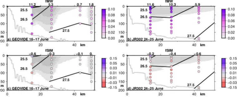
3.1. East Greenland Shelf
Figure 3 presents the SIM and MW fractions for the two eastern sections during Geovide (mid June [16–17 June]; left panels a and c) and JR302 (24–25 June; right panels b and d; see location in Figure 1). The spatial distribution offMWpresents a similar pattern for the two sections, with an increase shoreward and to the sur- face where there is freshening. We notice significantly higher MW fraction values on 24–25 June (maximum 0.11; Figure 1b) compared with the earlier 16–17 June section (maximum 0.08; Figure 1a). Interestingly, dur- ing Geovide there was an additional CTD cast done at 17 km, that is, 1.5 km further from the coast than the plotted inshore station. It presents higher salinity (often by 0.3) and warmer temperature, indicating large horizontal gradients. Thus, there might be even lower salinity/temperature and larger MW fractions closer to the coast than at the station at 15.5 km from the coast. So we suspect that the unsampled area inshore is rich in MW, with values as large as the ones observed at the JR302 station 14 km from shore. ForfSIM
(Figures 3b and 3d), positive values are only observed on both sections very close to the surface and mostly at the inner station. The strongerfSIMare observed in late June during JR302 (surface maximum of 0.03 at the innermost station). On both sections, negativefSIMvalues (−0.01/−0.02), indicating a signal of brines,
are observed near 100‐m depth. Notice that the brine signal is not present at the station ~52 km from the coast close to the shelf break, wherefSIMis close to 0. Furthermore, on Geovide section (left panel), the brine signal is not found already 26 km from the coast. Thus, all the negativefSIMvalues as well as the large MW fractions are within the EGCC based on the current data, whereas the outer stations on the shelf are outside the southwardflow of the EGCC.
The differences between the two sections suggest an offshore shift of the structure between the Geovide and JR302 sections, as well as a diminution of the surface peak velocities. Although there is a difference in bathy- metry between the two sections, it does not seem large enough to explain the shift, which is probably more the result of temporal evolution during the 8 days separating the two surveys, despite both sections being done in ice‐free water.
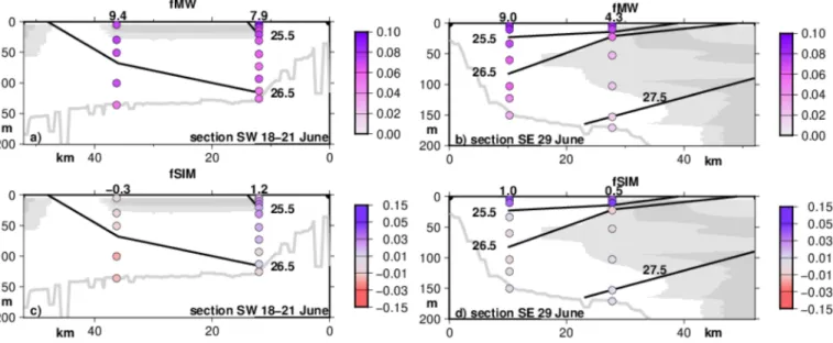
3.2. South of Cape Farewell
Figure 4 presents the freshwater distributions obtained from two sections located close to the southern tip of Cape Farewell, to its southwest and southeast. Similar to what we have discussed for the E sections, section SE (29 June) shows an increase shoreward and to the surface of MW fractions with strong values of 0.07–0.08 at the surface on the two innermost stations. Near‐zero MW fractions (Figure 4b) are calculated at ~67 km from the coast (after the shelf break; not shown). We calculated strong SIM inputs (fractions of 0.04–0.05) over the top 20 m of the two inner shelf stations, whereas subsurface samples show SIM fractions close to 0 (Figure 4d). On the S‐ADCP section taken just before the station (109) closest to shore, currents were weak and decreasing at subsurface towards the shore and with reversed currents at the surface and near bottom.
This section was taken during a short episode of strong southwesterly wind, which probably induced this near‐coastal current reversal. The strong baroclinicity is seen both in the isopycnal slope towards the coast and in the current profiles (not shown).
The left panels (section SW) of Figures 4a and 4c are based on stations located a bit further southwest of Cape Farewell and collected 8–11 days earlier than along section B. During the JR302 station located in front of the fjord estuary (21 June), strong SIM inputs (0.02–0.03) are observed down to 80 m (Figure 4c). MW are not particularly high at subsurface, whereas high MW fractions are only found at the surface with a maximal value of 0.09 (Figure 4a). The other station on the shelf, 36 km from the coast, was sampled a little earlier on 18 June during Geovide. It shows strong MW inputs (fMW= 0.07) down to 100 m and the presence of Figure 3.Spatial distribution along section E (left, Geovide; and right, JR302) offMWfractions (top [a, b] with water column inventories in meters reported on top of each station) andfSIM(bottom [c, d] with top 50‐m inventories in meters reported on top of each station). Thexaxis is the distance (kilometers) to the coast (the coast is to the west). Theyaxis is the depth (meters). The light‐gray line indicates the bottom depth from ETOPO1. The isopycnal contours for 25.5, 26.5, and 27.5 kg/m3are also sketched, as well as the cross‐track currents with gray shading for currents larger than 20 cm/s (darker grays for currents larger than 30 and 50 cm/s; those currents are southward and are not plotted west of the station closest to shore where they were not measured).
brines at subsurface (fSIM =−0.02). This station seems near the offshore edge of a weak coastal surface current, whereas the next station near the shelf break with weak MW and SIM fractions (not plotted) is already within the EGC.
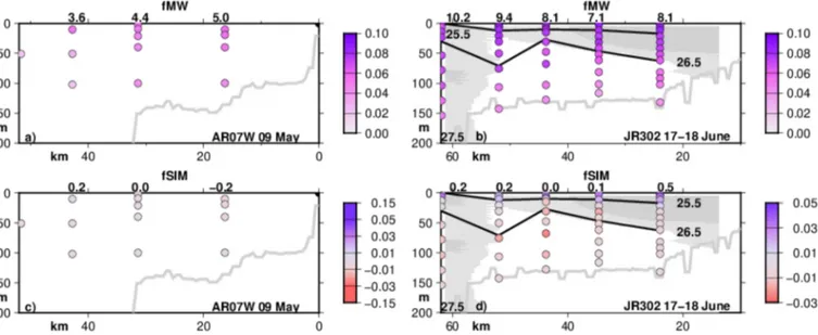
3.3. Southwest Greenland Shelf
Figure 5 presents the freshwater distributions obtained from the two sections located on the west side of Cape Farewell. The section HUD2014007 (AR07W) furthest to the west was sampled on 9 May before the core of the melt season. Distinctively from the previously discussed late spring sections, the MW and SIM distributions (Figures 5a and 5c) are uniform for the two shelf stations with values of 0.04–0.05 for MW and close to 0 for SIM. Potential density also presents little vertical or horizontal gradients on the shelf, with weak northwesterly currents presenting a slight maximum on the middle shelf.
For the JR302 section (17–18 June) located further south (Figures 5b and 5d), the MW contribution is close to that observed during AR07W at depth but increases toward the surface in the top 100 m. Positive SIM frac- tions are observed near the surface (0–25 m; Figure 5d). For MW and SIM, the fresh water extends across the full shelf instead of being only found in the inner part as is observed in the eastern sections discussed earlier.
At subsurface, negative values offSIM(−0.01 to−0.02) are found in the June section over the outer part of the shelf (at 44 and 52 km from the coast). Notice that the brines influence has a similar magnitude to the one observed on section SW (Figure 4c; 36 km from the coast). In both cases, they are also found outside of the branch of the northwestward current closest to the coast.
4. Discussion
The AR07W cruise (9 May) gives a snapshot of the freshwater distribution on the SW Greenland shelf downstream of Cape Farewell in an ice‐free sector before the onset of the 2014 melting season. At this time, the MW distribution appears rather homogeneous over the shelf, with integrated freshwater contents between 5.0 m (close to the coast) and 3.6 m (near shelf break). Moreover, SIM fraction values close to 0 suggest a balance at this time between SIM and sea ice formation (note that this result is sensitive to the choice of endmembers). The profiles are only weakly stratified (0.3 °C and 0.3 psu from top to bottom for the inner shelf station), which indicates that there was vertical mixing, as is typical of southwestern Greenland shelves in early spring.
Figure 4.Same as Figure 3 but for the two most southern sections (coast to the right for section SW and to the left for section SE). Section SW on the left to the southwest of Cape Farewell combines the inshore station of JR302 (21 June) and Geovide (18 June); section SE on the right to the southeast of Cape Farewell is from JR302 (lowered acoustic Doppler current profilers current at station closest to shore replaced by S‐ADCP currents taken just before arriving on station). Outer stations were cropped from the plots and present weakfMW(except just at the surface) andfSIM.
Then, in late spring 2014 from mid to late June, strong MW and SIM inputs are observed near the surface and on the shelf, with between 7‐and 11.5‐m total freshwater content on the southwestern shelf but also close to the coast east of Cape Farewell. The two near repeats of the eastern section E reveal that the freshwater variability can be strong at the synoptic time scale, with fast changes in the freshwater distribution to the EGC/EGCC system (~8 days between the two realizations of the section). A large part of the freshwater con- tent increases in JR302 relative to earlier Geovide E section could be explained by an outward displacement (by 15 km) or an increase in extent of the core of the EGCC, both being compatible with the observed current sections. In addition, during the later JR302 E section, there are also lower surface salinities (by at least 0.5), which could be contributed by an increase in SIM in the top 10 m but also by an increase in MW. However, because of the poor resolution of the large horizontal gradients, and also of the vertical gradients for Geovide, it is not possible to be quantitative. Nonetheless, the changes in MW and SIM (increase near the surface) are coincident with changes in the distribution of drifting sea ice according to ice maps, suggesting the possible arrival ofstoris(multiyear ice) originating from the Arctic, which is known to penetrate in this region in May–July (Schmith & Hansen, 2003). This might have been associated with the strong northeasterlies encountered during the JR302 repeat of the section on 24–25 June. Remnants of“old”sea ice were observed during some of the JR302 sections, indicating that we are also missing the component of the fresh water con- tained in thefloating ice. However, with the very low partial coverage, this component probably remains a very small contribution to the overall fresh water. Wind‐related changes in EGCC current and freshwater transport were also analyzed from a mooring array placed just afterwards (Le Bras et al., 2018) with day to day transport changes almost by a factor of 2. Large high frequency changes of the freshwater transport on the shelf were also commented from mooring data north of Denmark Strait (de Steur et al., 2017).
Most of the June 2014 sections suggest a subsurface signature of brines (near 100‐m depth) at some stations (fSIMof−2%). Along the east side of Cape Farewell, the brine signal at subsurface is close to the coast within the EGCC. It is further from the coast and closer to the shelf break for the sections to the southwest (section SW) and to the west of Cape Farewell. The brines are not found a week later on the two stations of the JR302 section located southeast of Cape Farewell (section SE). This might be either due the very low horizontal resolution of the section or due to synoptic changes in the shelf water masses in less than 10 days.
Synoptic changes in the water masses might have resulted from wind having then veered to the southeast, coincident with the current section showing the almost disappearance of the EGCC on the inner shelf.
Notice also that this brine signal is much lesser than what is described further upstream during summer cruises north of Denmark Strait (de Steur et al., 2015), indicating considerable changes in stratification and vertical mixing between the two latitudes.
Figure 5.Same as Figure 3 but for the western sections W (coast to the right). (a, c) The May AR07W section is to the left, and (b, d) the June JR302 section is to the right. No current velocity is plotted for AR07W.
While the strong MW influence is found in the inner part of the eastern Greenland shelf in the EGCC, the fresh water of MW or SIM origin isflowing towards the continental slope in the WGC current, spreading near the surface over the full shelf, as well as over the continental slope. For the southwest Greenland sec- tions, this is near the shelf break that the largest freshwater inventories are found, with values comparable to the ones on the inner shelf or the East Greenland sections. This difference/change from the eastern side of Cape Farewell to its western side noticed here both in near surface MW and SIM or in subsurface presence of brine‐marked water is coherent with observed separation of the EGCC core from the coast near Cape Farewell. See for example the available 15‐m drogue drifter trajectories (Global Drifter Program; Lumpkin et al., 2013), in particular the ones with largest velocities (Figure 6). This is also observed in earlier summer cruises (Holliday et al., 2007). This continuity of the freshwater content between the EGC and WGC has already been observed in the study of earlier cruises (Cox, 2010) during the years 2005 and 2008. This was also well described during one cruise with higher spatial resolution, which took place during the summer of 2014 (Lin et al., 2018), a few months after the surveys of this paper.
In the set of sections used here, the resolution is often insufficient to discuss whether the EGCC merges with the EGC or not on the southwestern sections. Indeed, the interruption of the subsurface brine presence (negative SIM fractions; Figure 4d) in section SE southeast of Cape Farewell suggests inadequate horizontal resolution, at least for that section. Interestingly, the current sections both from Geovide and JR302 suggest that a surface EGCC is still found near the coast to the southwest and west of Cape Farewell, albeit with a much weaker amplitude than to its east. Although this was not clearly identified during the May 2014 AR07W section, repeats of the AR07W section in other years that ended closer to shore (such as in 2016) also found a stronger surface EGCC close to shore. On the other hand, the presence of an EGCC on the south- western shelf in the 2014 spring surveys was not found in the late summer 2014 survey of Lin et al.
(2018). The large change of structure, stratification, and MW inventories between May and June was surpris- ing, even though the AR07W and JR302 are rather far apart. However, an earlier occurrence of AR07W in June 1995, which also had water isotopic data, presents a structure much closer to the June 2014 JR302 sec- tion than the May 2014 AR07W section. This suggests that there might be a large seasonal change in the water masses on this part of the shelf during this transitional season. The outward shift of the subsurface Figure 6.Drogue drifter trajectories (15 m) of the Global Drifter Program interpolated at a 6‐hr time step (Atlantic Oceanographic and Meteorological Laboratory Global Drifter Program Global Data Assembly Center site). The red color corresponds to velocities larger than 40 cm/s (and blue color for lower velocities). The 100‐, 300‐, and 500‐m isobaths are outlined (black contours). AOML GDP GDAC = Atlantic Oceanographic and Meteorological Laboratory Global Drifter Program GlobalData Assembly Center.
brine signal between the eastern and the western June 2014 JR302 sections is also indicative, that at least below 50 m, the EGCC joins the EGC closer to the shelf break between the two sections.
There is another anomaly that needs to be commented, which is that the JR302 station located in front of the fjord system (near Narsarmijit) on section SW (Figure 4a and 4c) shows an unusual deep influence of SIM in the water column. The strong vertical mixing could be due to fjord processes in the presence of strong winds and tides, as this fjord system also connects with east Greenland and includes many inlets, islands, and sills.
Notice that for this station, MW inputs are not particularly high, compared to the strong SIM values, suggest- ing that at this time and in the fjord system, SIM contribution is important relative to the MW inputs. It is also possible that a local contribution of meltwater in this fjord with a less negativeδ18O isotope value than what we use could be mistaken as excess positive SIM.
The supporting information discusses whether another approach on partitioning fresh water using TA data could be used to complement the study. At this point, and although there is a promising correlation between estimates of the two approaches, the approach using alkalinity seems to be underconstrained. This is possibly due to contributions from unconsidered biological processes and of the interaction between elements in solid and in dissolved forms that modify TA, as particles have been found to be in rather large quantity in the inner shelf station of the Geovide cruise (Tonnard et al., 2018). Indeed, two JR302 stations with alkalinity (but no water isotope) data also provide a very striking deviation from what is expected, that we attribute to massive particle influx, possibly from melting sea ice. This could also be the signature of particularly alkaline spring polar water, as has been observed in early spring further north on the east Greenland shelf (Nondal et al., 2009). Interestingly, this water is not observed at other sections from the JR302 cruise. Thus, for those other sections, it was either trapped closer to the shore than thefirst station, or its presence in this region is highly intermittent. Furthermore, this was not found near southeast Greenland in the Global Ocean Data Analysis Project hydrographic station database (Olsen et al., 2016) nor in any of the eight late spring OVIDE cruises (between 2002 and 2016; the 2014 cruise being the Geovide cruise of this paper; Perez et al. (2018)).
5. Conclusion and Perspectives
This study was aimed at investigating the origin of fresh water on the shelves near Cape Farewell during the late spring 2014. This was done with a simple partitioning between MW sources and SIM or brine formation.
We benefited from a set of three cruises, which illustrate the time variability of freshwater input. We clearly see a strong increase in MW in the shelf upper layer (by nearly a factor 2 or 4.5 m) between the May and late June season spanned by the three cruises that likely results from east Greenland melting. There was also a contribution of SIM near the surface but with large spatial variability as well as temporal variability between the two June cruises. Furthermore, gradients in the freshwater distribution are larger east of Cape Farewell than west of Cape Farewell, which is related to the EGCC being more intense and closer to the coast east of Cape Farewell than west of it. Also, we observed a weaker surface‐intensified EGCC southwest and west of Cape Farewell on the shelf on all sections.
We also found a subsurface brine signal that tracks the EGCC subsurface pathway. During these mid to late June surveys, it is found close to the coast east of Cape Farewell but closer to the shelf break west of Cape Farewell. This brine signal is unlikely to be an artifact of our identification of endmembers. It probably acquires its signature upstream on the east Greenland shelf or further north during the previous winter when winter ice forms over a mixed layer reaching 50‐to 100‐m thickness. On the other hand, part of the variability near the surface both in time and in space could be related to different sources of MW (snow melt vs. glacier melt or different glaciers or in the Arctic). A quantitative investigation would require higher spa- tial resolution during the cruises, in addition to characterizing the current variability and better identifying the different sources. The EGCC, in particular, is a rather narrow structure (core of 10–20‐km width) with a complicated path in this region (Holliday et al., 2007; Lin et al., 2018), which was not sufficiently resolved during these cruises. For example, a strong variability inTandSvertical profiles has been observed between different casts of the Geovide station closest to Greenland along section E, which are only 1–2 km apart. The differences between the two near repeats of the eastern section (Geovide and JR302) seem more large scale and could be either associated with a shift of the EGCC core away from the coast or an increase in its exten- sion, together with a decrease of its surface intensity. We expect that the differences between these two near repeats of section E or with section B a little further south are associated with the different wind conditions encountered and the associated response of the near‐coastal ocean, as suggested by mooring data a little
more than 10 km from the coast along section E (Le Bras et al., 2018). We speculate that this mooring could miss a significant part of the freshwater transport during the later spring to early summer season due to the very fresh water and currents trapped sometimes very close to the coast and the sea surface, which could not be measured by this mooring. Furthermore, although the current was well measured on this mooring, there are more data gaps in the salinity records, and complementary measurements should be sought to comple- ment its valuable records.
The sensitivity of the results to the particular sampling during these cruises could be investigated/examined using eddy‐resolving simulations with well resolved source waters along eastern and southeastern Greenland. We expect large seasonal freshwater variability in this region (Bacon et al., 2014), as also observed from mooring data (Le Bras et al., 2018); and thus, it is not surprising that there are significant differences with other surveys and sections that took place later in summer and early autumn (Cox et al., 2010;
Sutherland et al., 2009). For example, the brine signal that we observed in June 2014 at depth is only found once in these published surveys. In late summer, there might also be less influence of local freshwater sources and drifting sea ice, thus a more direct connection to higher latitudes or at least more integrated and less local.
Further upstream, near Denmark Strait, there has been evidence for large recent interannual variability in the freshwater composition (de Steur et al., 2015). How this signal can be detected downstream, and isolated from the fast variability found, at least during the spring surveys of the present study, needs to be further investigated.
Data Availability Statement
Most of the hydrographic data will be available on the CCHDO website (hydrography and nutrients) in the near future. Geovide hydrographic and current data are available (Lherminier & Sarthou, 2017). The isotopic data were submitted to the free Global Seawater Oxygen‐18 Database. The S‐ADCP data of Geovide are avail- able at Lherminier and Sarthou (2017). The Geovide bottle data are available on SEANOE (https://doi.org/
10.17882/54653). An update is done (summer 2019) to include additional variables includingδ18O. All the δ18O data have been transferred to GISS to be archived in“Global Seawater Oxygen‐18 Database”(https://
data.giss.nasa.gov/o18data/;Schmidt et al., 1999). The JR302 CTD, bottle, and ADCP data are available from BODC (https://www.bodc.ac.uk/resources/inventories/cruise_inventory/report/15037/). The bottle data for AR07W (HUD2014007) are at CCHDO.
References
Bacon, S., Marshall, A., Holliday, N. P., Aksenov, Y., & Dye, S. R. (2014). Seasonal variability of the East Greenland coastal current.Journal of Geophysical Research: Oceans,119, 3967–3987. https://doi.org/10.1002/2013JC009279
Bacon, S., Reverdin, G., Rigor, I. G., & Snaith, H. M. (2002). A freshwater jet on the east Greenland shelf.Journal of Geophysical Research, 107(C7), 3068. https://doi.org/10.1029/2001JC000935
Belkin, I. M. (2004). Propagation of the“Great Salinity Anomaly”of the 1990s around the northern North Atlantic.Geophysical Research Letters,31, L08306. https://doi.org/10.1029/2003GL019334
Belkin, I. M., Levitus, S., Antonov, J., & Malmberg, S. A. (1998).“Great salinity anomalies”in the North Atlantic.Progress in Oceanography, 41(1), 1–68. https://doi.org/10.1016/S0079‐6611(98)00015‐9
Benetti, M., Reverdin, G., Lique, C., Yashayaev, I., Holliday, N. P., Tynan, E., et al. (2017). Composition of freshwater in the spring of 2014 on the southern Labrador shelf and slope.Journal of Geophysical Research: Oceans,122, 1102–1121. https://doi.org/10.1002/2016JC012244 Benetti, M., Reverdin, G., Pierre, C., Khatiwala, S., Tournadre, B., Olafsdottir, S., & Naamar, A. (2016). Variability of sea ice melt and
meteoric water input in the surface Labrador Current off Newfoundland.Journal of Geophysical Research: Oceans,121, 2841–2855.
https://doi.org/10.1002/2015JC011302
Benetti, M., Sveinbjörnsdóttir, A. E., Ólafsdóttir, R., Leng, M. J., Arrowsmith, C., Debondt, K., et al. (2017). Inter‐comparison of salt effect correction forδ18O andδ2H measurements in seawater by CRDS and IRMS using the gas‐H2O equilibration method.Marine Chemistry, 194, 114–123. https://doi.org/10.1016/j.marchem.2017.05.010
Cox, K. A. (2010). Stable isotopes as tracers for freshwaterfluxes into the North Atlantic.University of Southampton, School of Ocean and Earth Science, Doctoral Thesis, 178 pp.
Cox, K. A., Staford, J. D., McVicar, A. J., Rohling, E. J., Heywood, K. J., Bacon, S., et al. (2010). Interannual variability of Arctic Sea ice export into the East Greenland Current.Journal of Geophysical Research,115, C12603. https://doi.org/10.1029/2010JC006227 Curry, R., & Mauritzen, C. (2005). Dilution of the northern North Atlantic Ocean in recent decades.Science,308(5729), 1772–1774. https://
doi.org/10.1126/science.1109477
de Steur, L., Pickart, R. S., Macrander, A., Våge, K., Harden, B., Jonsson, S., et al. (2017). Liquid freshwater transport estimates from the East Greenland Current based on continuous measurements north of Denmark Strait.Journal of Geophysical Research: Oceans,122, 93–109. https://doi.org/10.1002/2016JC012106
de Steur, L., Pickart, R. S., Torres, D. J., & Valdimarsson, H. (2015). Recent changes in the freshwater composition east of Greenland.
Geophysical Research Letters,42, 2326–2332. https://doi.org/10.1002/2014GL062759
Dickson, R., Rudels, B., Dye, S., Karcher, M., Meincke, J., & Yashayaev, I. (2007). Current estimates of freshwaterflux through Arctic and subarctic seas.Progress in Oceanography,73(3‐4), 210–230. https://doi.org/10.1016/j.pocean.2006.12.003
Acknowledgments
The authors would like to thank Mark Stinchcombe, Hannah Donald, and Carolyn Graves for collecting the nutrient data used in this work. The authors are also indebted to the isotope lab and the other institutions that made their data available for the work. J. C.
was funded under The Analytical Chemistry Trust Fund, funded by the Royal Society for Chemistry and the UK Natural Environment Research Council (NE/I019638/1) and GEOMAR. E. T.
was funded by RAGNARROC. M. B.
was funded by the University of Iceland with support by the National Power Company of Iceland Landsvirkjun. The authors would also like to thank Matthew Humphreys, Claudia Fry, and Alex Griffiths for their help in analyz- ing and collecting the samples. The Geovide cruise research was funded by the French National Research Agency (ANR‐13‐BS06‐0014), the French National Center for Scientific Research (CNRS‐LEFE‐CYBER), and Ifremer. A special thank is also due to the R/V
“Pourquoi Pas?”crew and Captain G.
Ferrand, to Géraldine Sarthou for her help, and to Arni Sveinbjörnsdottir for her encouragements. JR302 and authors N. P. H., E. T., and STV were funded by NERC projects UK OSNAP (NE/K010875/1), RAGNARROCC (NE/K002511/1), and the Extended Ellett Line (National Capability), respectively. We gratefully acknowl- edge the Atlantic Zone Off‐Shelf Monitoring Program (AZOMP) of Fisheries and Oceans Canada (DFO;
http://www.bio.gc.ca/science/monitor- ing‐monitorage/azomp‐pmzao/azomp‐ pmzao‐en.php), including its partici- pants and crew of CCGS Hudson.
Dickson, R. R., Meincke, J., Malmberg, S. A., & Lee, A. J. (1988). The“great salinity anomaly”in the northern North Atlantic 1968–1982.
Progress in Oceanography,20(2), 103–151. https://doi.org/10.1016/0079‐6611(88)90049‐3
Dodd, P. A., Heywood, K. J., Meredith, M. P., Naveira‐Garabato, A. C., Marca, A. D., & Falkner, K. K. (2009). Sources and fate of freshwater exported in the East Greenland Current.Geophysical Research Letters,36, L19608. https://doi.org/10.1029/2009GL039663
Fry, C. H., Tyrrell, T., Hain, M. P., Bates, N. R., & Achterberg, E. P. (2015). Analysis of global surface ocean alkalinity to determine con- trolling processes.Marine Chemistry,174, 46–57. https://doi.org/10.1016/j.marchem.2015.05.003
Hansen, B., & Østerhus, S. (2000). North Atlantic‐Nordic Seas exchanges.Progress in Oceanography,45(2), 109–208. https://doi.org/
10.1016/S0079‐6611(99)00052‐X
Holliday, N. P., Bacon, S., Cunningham, S. A., Gary, S. F., Karstensen, J., King, B. A., et al. (2018). Subpolar North Atlantic overturning and gyre‐scale circulation in the summers of 2014 and 2016.Journal of Geophysical Research: Oceans,123, 4538–4559. https://doi.org/
10.1029/2018JC013841
Holliday, N. P., Meyer, A., Bacon, S., Alderson, S. G., & de Cuevas, B. (2007). Retroflection of part of the east Greenland Current at Cape Farewell.Geophysical Research Letters,34, L07609. https://doi.org/10.1029/2006GL029085
Jeansson, E., Jutterström, S., Rudels, B., Anderson, L. G., Olsson, K. A., Jones, E. P., et al. (2008). Sources to the East Greenland Current and its contribution to the Denmark Strait overflow.Progress in Oceanography,78(1), 12–28. https://doi.org/10.1016/j.pocean.2007.08.031 King, B. A., & Holliday, N. P. (2015). RRS James Clark Ross cruise 302, 06 Jun‐21 Jul 2014, The 2015 RAGNARRoC, OSNAP and Extended
Ellett Line cruise report, National Oceanography Centre Southampton: 76.
Latif, M., Böning, C., Willebrand, J., Biastoch, A., Dengg, J., Keenlyside, N., et al. (2006). Is the thermohaline circulation changing?Journal of Climate,19(18), 4631–4637. https://doi.org/10.1175/JCLI3876.1
Lazier, J. R. N. (1973). The renewal of Labrador Sea water,Deep Sea Research and Oceanographic Abstracts, Vol. 20, 341–353. https://doi.
org/10.1016/0011‐7471(73)90058‐2
Le Bras, I. A.‐A., Straneo, F., Holte, J., & Holliday, N. P. (2018). Seasonality of freshwater in the East Greenland Current system from 2014 to 2016.Journal of Geophysical Research: Oceans,123, 8828–8848. https://doi.org/10.1029/2018JC014511
Lherminier P., & Sarthou, G. (2017). The 2014 Greenland‐Portugal GEOVIDE CTDO2 hydrographic and SADCP data (GO‐SHIP A25 and GEOTRACES GA01). SEANOE. https://doi.org/10.17882/52153
Lin, P., Pickart, R. S., Torres, D. J., & Pacini, A. (2018). Evolution of the freshwater coastal current at the southern tip of Greenland.Journal of Physical Oceanography,48, 2128–2140. https://doi.org/10.1175/JPO‐D‐18‐0035.1
Lumpkin, R., Grodsky, S. A., Centurioni, L., Rio, M.‐H., Carton, J. A., & Lee, D. (2013). Removing spurious low‐frequency variability in drifter velocities.Journal of Atmospheric and Oceanic Technology,30, 353–360. https://doi.org/10.1175/JTECH‐D‐12‐00139.1 Luo, H., Castelao, R. M., Rennermalm, A. K., Tedesco, M., Bracco, A., Yager, P. L., & Mote, T. L. (2016). Oceanic transport of surface
meltwater from the southern Greenland ice sheet.Nature Geoscience,9(7), 528–532. https://doi.org/10.1038/NGE2708 Mintrop, L., Perez, F. F., Gonzalez‐Davila, M., & Santana‐Casanio, J. M. (2000). Alkalinity determination by potentiometry:
Intercalibration using three different methods.Ciencias Marinas,26, 23–37. https://doi.org/10.7773/cm.v26i1.573
Nondal, G., Belerby, R. G. J., Olsen, A., Johannessen, T., & Olafsson, J. (2009). Optimal evaluation of the surface ocean CO2 system in the northern North Atlantic using data from voluntary observing ships.Limnology and Oceanography: Methods,7(1), 109–118. https://doi.
org/10.4319/lom.2009.7.109
Olsen, A., Key, R. M., van Heuven, S., Lauvset, S. K., Velo, A., Lin, X., et al. (2016). The Global Ocean Data Analysis Project version 2 (GLODAPv2)‐An internally consistent data product for the world ocean.Earth System Science Data,8(2), 297–323. https://doi.org/
10.5194/essd‐8‐297‐2016
Östlund, H. G., & Hut, G. (1984). Arctic Ocean water mass balance from isotope data.Journal of Geophysical Research,89(C4), 6373–6381.
https://doi.org/10.1029/JC089iC04p06373
Perez, F. F., Fontela, M., Garcia‐IBanez, M. I., Mercier, H., Velo, A., Lherminier, P., et al. (2018). Meridional overturning circulation conveys fast acidification of the deep Atlantic Ocean.Nature,554(7693), 515–518 (22 February 2018. https://doi.org/10.1038/
nature25493
Pickart, R. S., Torres, D. J., & Fratantoni, P. S. (2005). The East Greenland spill jet.Journal of Physical Oceanography,35(6), 1037–1053.
https://doi.org/10.1175/JPO2734.1
Sarthou G., & Lherminier, P. (2014). GEOVIDE cruise, RV Pourquoi pas?, https://doi.org/10.17600/14000200
Schmidt, G.A., G. R. Bigg, & E. J. Rohling. (1999).“Global Seawater Oxygen‐18 Database‐v1.22”https://data.giss.nasa.gov/o18data/
Schmith, T., & Hansen, C. (2003). Fram Strait ice export during the nineteenth and twentieth centuries reconstructed from a multiyear sea ice index from southwestern Greenland.Journal of Climate,16(16), 2782–2791. https://doi.org/10.1175/1520‐0442(2003)016<2782:
FSIEDT>2.0.CO;2
Shepherd, A., Ivins, E. R., Geruo, A., Barletta, V. R., Bentley, M. J., Bettadpur, S., et al. (2012). A reconciled estimate of ice‐sheet mass balance.Science,338(6111), 1183–1189. https://doi.org/10.1126/science.1228102
Skrzypek, G., & Ford, D. (2014). Stable isotope analysis of saline water samples on a cavity ring‐down spectroscopy instrument.
Environmental Science & Technology,48, 2827–34. https://doi.org/10.1021/es4049412
Sofer, Z., & Gat, J. R. (1972). Activities and concentrations of oxygen‐18 in concentrated aqueous salt solutions: Analytical and geophysical implications.Earth and Planetary Science Letters,15(3), 232–238. https://doi.org/10.1016/0012‐821X(72)90168‐9
Stanford, J. D., Rohling, E. J., Bacon, S., & Holliday, N. P. (2011). A review of the deep and surface currents around Eirik Drift, south of Greenland: Comparison of the past with the present.Global and Planetary Change,79, 244–254. https://doi.org/10.1016/j.
gloplacha.2011.02.001
Sutherland, D. A., & Pickart, R. S. (2008). The East Greenland Coastal Current: Structure, variability, and forcing.Progress in Oceanography,78(1), 58–77. https://doi.org/10.1016/j.pocean.2007.09.006
Sutherland, D. A., Pickart, R. S., Peter Jones, E., Azetsu‐Scott, K., Jane Eert, A., & Ólafsson, J. (2009). Freshwater composition of the waters off southeast Greenland and their link to the Arctic Ocean.Journal of Geophysical Research,114, C05020. https://doi.org/10.1029/
2008JC004808
Tesdal, J. E., Abernathey, R. P., Goes, J. I., Gordon, A. L., & Haine, T. W. (2018). Salinity trends within the upper layers of the subpolar North Atlantic.Journal of Climate,31(7), 2675–2698. https://doi.org/10.1175/JCLI‐D‐17‐0532.1
Tonnard, M., H. Planquette, A. R. Bowie, P. van der Merwe, M. Gallinari, F. Desprez de Gésincourt, et al. (2018). Dissolved iron in the North Atlantic Ocean and Labrador Sea along the Geovide section (GEOTRACES section GA01).Biogeosciences Discussions, https://doi.org/
10.5194/bg‐2018‐147
Yashayaev, I., van Aken, H. M., Holliday, N. P., & Bersch, M. (2007). Transformation of the Labrador Sea water in the subpolar North Atlantic.Geophysical Research Letters,34, L22605. https://doi.org/10.1029/2007GL031812