on the Northeast Greenland Shelf

(1)

M

ASTER

T

HESIS

Benthic Soft-bottom Communities and Ecosystem Functions

on the Northeast Greenland Shelf

Yasemin Bodur

1st Examiner:

Prof. Dr. Thomas Brey¹ 2nd Examiner:

Dr. Ulrike Braeckman²

1Alfred Wegener Institute, Helmholtz Centre for Polar and Marine Research, Germany

2Ghent University, Marine Biology Research Group, Belgium

A thesis submitted in fulfillment of the requirements for the degree ofMaster of Science

September 25, 2018

(2)

(3)

“For the game of Western philosophy and science is to trap the universe in the networks of words and numbers, so that there is always the temptation to confuse the rules, or laws, of grammar and mathematics with the actual operations of nature. [...] every thing-event is what it is only in relation to all others. ”

Alan Watts, Tao: The Watercourse Way

(4)

(5)

List of Figures

1.1 Schematic illustration of pelagic-benthic coupling. . . 2

2.1 Bathymetry and geographical names in the study area on the NEG shelf. 6 2.2 Schematic illustration of inferred water mass pathways on the NEG shelf. . . 7

2.3 Locations of sampling sites on the NEG shelf during PS109 onR/V Polarstern in September/October 2017. . . 8

3.1 Variation of CPE with sediment depth. . . 20

3.2 Dotplots of environmental parameters from ex situ and in situ samples. 21 3.3 Bottom water potential temperature and salinity at benthic stations. . . 22

3.4 GAM-smoothed attenuation profiles. . . 22

3.5 Dotplots for oxygen fluxes and bottom water nutrient concentrations. . 24

3.6 Sediment nutrient and DIC profiles. . . 25

3.7 Correlation plot of Spearman-rank correlations. . . 27

3.8 Principal component analysis (PCA) showing similarity among stations based on environmental variables. . . 29

3.9 Species accumulation curves for macrofauna species from ex situ samples. . . 31

3.10 Dotplots for community parameters and single cell abundances. . . 31

3.11 The most important phyla sampled at each site. . . 33

3.12 Diversity indices based on community abundances for each site. . . 34

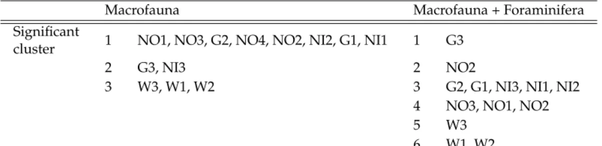
3.13 Dendrogram representation of the results of Bray-Curtis distances- based SIMPROF analysis. . . 36

3.14 nMDS plot on squareroot-transformed polychaeta with the twelve most abundant families. . . 37

3.15 Visualisation of the Correspondance analysis (CA) results on ex situ community density with fitted environmental parameters. . . 38

3.16 CPE and total macrofauna density in 1992 and 2017. . . 42

A.1 Locations of the stations at the glacier front with detailed bathymetry. 75 A.2 Temperature and salinity profiles along a section within the trough system on the NEG shelf. . . 76

A.3 Uncalibrated raw fluoromenter values from the CTD during PS109 in the upper 200 meters. . . 76

A.4 Bottom water temperature and salinity from PS25 and PS109. . . 77

A.5 Sea ice conditions on 14th of September, 2017 during PS109. . . 77

A.6 Bottom water current velocities and temperatures. . . 78

A.7 Attenuation and chlorophyll a concentrations. . . 78

(8)

(9)

List of Tables

2.1 Metadata for the benthic stations on the NEG shelf during PS109. . . . 9 3.1 Correlation coefficients for Spearman rank correlations. . . 28 3.2 Principal Component Analysis results of standardized environmental

variables. . . 29 3.3 Benthic community parameters for all stations at the NEG shelf. . . 32 3.4 Results of Bray-Curtis distances-based SIMPROF analysis. . . 35 3.5 Results of the correspondence analysis (CA) on ex situ community

density. . . 39 3.6 one-way PERMANOVA results of Bray-Curtis distance based commu-

nity abundance matrices. . . 39 3.7 Results of multilevel pairwise comparisons among groups (locations)

on Bray-Curtis distances based community data. . . 40 3.8 Bray-Curtis distance based linear model of macrofauna + foraminifera

densities against environmental drivers. . . 41 3.9 Results of two-way ANOVA and Tukey HSD pairwise comparison test

for differences in macrofauna total density and CPE concentrations among regions and time. . . 41 A.1 Environmental parameters and TOU for each station. . . 79 A.2 Modelled mean porosity per sediment depth from silt fraction. . . 80 A.3 List of macrofauna taxa on the NEG shelf sampled during PS109. . . . 81

(10)

(11)

List of Abbreviations

79NG 79N Glacier; Nioghalvfjerdsbrae ADCP Acoustic Doppler Current Profiler AIW Atlantic Intermediate Water

AW Atlantic Water

CA Correspondence Analysis

CCA Canonical Correspondence Analysis

Chla Chlorophylla

CPE Chloroplastic pigment equivalent (Chlorophyllaand Phaeopigments) CTD Conductivity, Temperature, Depth prolifer

DCA Detrendend Correspondence Analysis DIC dissolved inorganic carbon

DOU diffusive oxygen uptake

EGC East Greenland Current

GAM Generalized Additive Model

KW Knee Water

mAIW glacially modified Atlantic Intermediate Water (TV-) MUC (TV-) Multicorer

NEG Northeast Greenland

NEGIS Northeast Greenland Ice Sheet

NEW Northeast Water

NØIB Norske Øer Ice Barrier

nMDS non-metric multidimensional scaling

OM organic matter

PERMANOVA permutational analysis of variance pers. comm. personal communication

PW Polar Water

SCA single cell abundance

SIMPROF similarity profile routine analysis

TA Total Alkalinity

TOU total oxygen uptake

(12)

(13)

Benthic communities regulate numerous ecosystem processes and rely almost exclusively on the sinking of organic matter from the pelagic. In association with climate change the Arctic sea ice is shrinking, glacial discharge is increasing and Arctic marine ecosystems are expected to become more Atlantic in character. For the last 20 years, these environmental changes were observed for the Northeast Greenland (NEG) shelf and might have altered benthic community structures and their function in this region. In September/October 2017, soft-bottom communities were sampled and oxygen consumption was measured ex situ over time at 13 stations on the NEG shelf. Sediment granulometry and porosity, pigment concentrations and porewater chemistry (DIC, nutrients, sulfate, chloride) were assessed to characterize the habitat.

It was found that macrofauna communities did not separate among regions, while foraminifera communities (>500µm) and polychaeta did distinguish the northern Westwind Trough from the southern Norske Trough and the 79N Glacier. Benthic pigment concentration was the most important predictor for the community structure.

Total abundance and biomass of macrofauna, single cell abundances, porewater DIC and ammonia concentrations were highest in the Westwind Trough compared to all other regions, which suggests the highest benthic productivity in the Westwind Trough. Overall benthic pigment concentrations were up to sevenfold lower compared to the 1990s, accompanied by a fivefold lower total abundance of macrofauna.

The present study confirms previous reports about a strong pelagic-benthic coupling on the NEG shelf which might have weakened since the 1990s, suggesting that this is a result of higher zooplankton grazing. Longer ice-free periods and higher inflow of warm Atlantic Water on the NEG shelf might have led to favourable conditions for zooplankton of Atlantic origin, increasing pelagic mineralization that would finally lead to a reductrion in the amount of organic matter reaching the sea floor.

Keywords:sediment, nutrients, infauna, NEW Polynya

(14)

(15)

1 Introduction

1.1 Climate change and Arctic benthos

As a result of climate change, polar regions are warming more than any other region on earth (Turner and Marshall,2011). In the Arctic, the summer sea ice extent is declining at a rate that the region could be left ice-free in summer by the middle of this century (IPCC,2013). Enhanced glacial melt, especially at Greenland’s glaciers (Rignot and Kanagaratnam,2006;Nick et al.,2013) and the shifting of warming water masses towards the high North (Beszczynska-Möller et al.,2012) are further effects that come along with climate change. This will most likely lead to drastic changes in Arctic ecosystems through all trophic levels.

Marine ecosystems in the Arctic are characterized by extreme seasonal changes in light availability and primary production due to seasonal sea ice dynamics (Leu et al.,2015). Pelagic mineralization patterns determine the amount of Organic Matter (OM) that sinks to the sea floor and ultimately serves as food for benthic communities (Graf,1989;Wassmann and Reigstad,2011). This has an impact on benthic functions and processes (Morata et al.,2015). A strong dependency of benthic ecosystems on pelagic processes in the Arctic (i.e. "pelagic-benthic coupling"; Fig. 1.1) has been documented for various fjord (e.g.McMahon et al.,2006) and shelf systems (Link et al.,2013;McTigue et al.,2015) as well as for the deep Arctic Ocean (Degen et al., 2015).

Several scenarios are discussed for the consequences of shrinking sea ice regarding primary production and with that on the fate of OM reaching the sea floor (Wassmann and Reigstad,2011). A longer period of light availability might fuel more pelagic phytoplankton blooms (Arrigo et al.,2008), but the establishment of a bloom depends on multiple factors such as nutrient availability, vertical mixing and the amount of wind stress (Ardyna et al.,2014). These factors can be further influenced by sea ice loss and might affect primary production in a negative or positive way, depending on the region.

Moreover, primary production is determined by sea ice algae and pelagic phytoplankton in concert, whereby sea ice algae can contribute in a high amount to spring primary production (Horner and Schrader,1982). Sea ice algae are regarded as a food source with higher nutritional value (Falk-Petersen et al.,1998). With a shorter sea ice season during the year, contribution to OM from both sources should shift towards phytoplankton, altering the quality and quantity of food reaching the benthos (Smith et al.,2013;Mäkelä et al.,2017b;Braeckman et al.,2018).

In the vicinity of glaciers, benthic communities are additionally influenced by glacial activity. Glacial meltwater input influences directly the physical dynamics of the water e.g. in terms of water column stratification, salinity and temperature as well as nearshore turbidity which in turn inhibits primary production at the surface due to the lower light availability (Görlich et al.,1987;Dierssen et al.,2002). Organisms at glacier proximities are subject to chronic physical disturbance and experience

(16)

FIGURE1.1:Schematic illustration of pelagic-benthic coupling.Organic matter sinking down from the upper water column, induced by primary production, determines the composition and amount of food (pigments) that is available for benthic communities. This study focused onmacrofaunaand microorganisms(single cell abundances) as components of the benthic community. They take upoxygen during the consumption of food. By their activity,nutrientsget remineralized, which is an important function of the benthos. Environmental parameters, e.g.grain sizeand water properties (temperature &

salinity) can influence the distribution and functioning of benthic comminities (M. Bodur).

low food input (Gutt,2001;Włodarska-Kowalczuk and Pearson,2004;Renaud et al., 2007b). Therefore, rather small and/or motile surface deposit-feeders or predators are mainly observed near glaciers (Włodarska-Kowalczuk et al.,2005;Renaud et al., 2007b;Pasotti et al.,2015) and species diversity is usually low (Włodarska-Kowalczuk et al.,2005;Renaud et al.,2007b;Pasotti et al.,2015).

Depending on wind and water circulation patterns, marine terminating glaciers may be important for marine productivity due to the initiation of nutrient upwelling (Meire et al.,2017;Hopwood et al., 2018), or may enhance stratification in fjords, counteracting primary production (van de Poll et al., 2018). Recently, the mass losses of the Greenland ice sheet quadrupled from 51± 65Gtyr⁻¹ (1992-2000) to 211±37Gtyr⁻¹(2000-2011;Shepherd et al.,2012). Especially the marine tidewater glaciers are subject to rapid retreats (Moon and Joughin,2008), and their transformation into land-terminating glaciers is likely (Meire et al.,2017), which could have effects on the structure and functions of benthic communities (Pasotti et al.,2015).

Another important feature that may alter benthic communities in the Arctic is the flow of warm Atlantic water towards the Arctic Ocean (´Slubowska et al.,2005;

Beszczynska-Möller et al.,2012). If Atlantic water will warm further, Arctic regimes may become more Atlantic in character (Cochrane et al.,2009). The introduction of species from the Atlantic can alter the benthic community composition, and finally the functioning of benthic ecosystems. A shift of Atlantic species further North is

(17)

ongoing across all trophic levels (e.g.Drinkwater,2006;Fleischer et al.,2007;Hegseth and Sundfjord,2008;Gregory et al.,2009;Kortsch et al.,2012;Braeckman et al.,2018).

A "borealization" of Arctic benthic communities is seen in fjord systems around Sval- bard (Kortsch et al.,2012) and in the Northern Bering Sea (Grebmeier et al.,2006).

Predation pressure could change through the introduction of higher trophic animals.

Zooplankton communities that are adapted to longer time of food availability might alter the tightness of the pelagic-benthic coupling through their grazing activities (Olli et al.,2007).

1.2 The importance of benthic communities in marine sys- tems

The amount of OM that is exported vertically varies regionally. On average, only a small fraction of the primary production (< 5%) is settling to the sea floor, serving as food for the benthos (Schlüter et al.,2000). Pelagic processes, both biological (zooplankton grazing, microbial recycling) or physical (e.g. lateral advection) influence this export (Grebmeier and Barry,1991). Microorganisms, single celled protists (especially foraminifera) and metazoans together constitute benthic communities. These are broadly distinguished according to their size (meiofauna, 0.02−₁mm; macrofauna, 0.5−20mmand megafauna> 20mm) and their ecological niche (infauna and epifauna). Benthic communities regulate numerous ecosystem processes such as carbon uptake, nutrient cycling (Link et al.,2013), oxygen respiration, organic matter decomposition, carbon burial and bioturbation (Clough et al.,1997). They deliver an important food source for e.g. marine mammals (Grebmeier et al.,2006). Opposing a common statement that the Arctic benthos is species-poor, it is, globally seen, rather characterized by intermediate diversity (Piepenburg et al.,2011).

In infaunal communities, polychaetes are usually the most abundant taxon (Hartmann-Schröder, 1996). They are regarded as good predictors of variability in Arctic macrobenthic communities (Włodarska-Kowalczuk and Kedra,2007). The same was observed for foraminifera (Włodarska-Kowalczuk and Kedra,2007;Mo- jtahid et al.,2008;Denoyelle et al.,2010). Foraminifera are important components of benthic communities and can account sometimes for 50 % or more of eukary- otic biomass (Gooday et al.,1992). Studies in polar regions that comprise several fractions of benthic communities and relate their distribution patterns to prevailing environmental drivers are rare (e.g.Piepenburg et al.,1997;Włodarska-Kowalczuk et al., 2013; Pasotti et al., 2015). Usually, investigations concentrate on only one fraction because the spanning of all size ranges is extremely elaborate, costly and time-consuming. However, it is necessary to get the full picture of the functioning of benthic communities.

1.3 The NE Greenland Shelf - case example for a changing Arctic

The Northeast Greenland Ice Sheet (NEGIS) is the largest part of the Greenland Ice Sheet. While the glaciers of Southeast and Northwest Greenland are subject to strong mass losses, the northern sector exhibited a small loss for a long time (Rignot and Kanagaratnam,2006). However, starting between 2003 and 2006, glaciers around Northeast Greenland undergo sustained dynamic thinning (Khan et al.,2014). The

(18)

melting is probably triggered by increasing air temperature and the resulting reduced sea-ice concentration (Khan et al.,2014) which normally suppresses calving front retreat (Nick et al.,2012) and/or rising ocean temperatures (Mouginot et al.,2015).

The Northeast Greenland (NEG) shelf is located in the high Arctic between 77°and 81°N. Glacial melt, shrinking sea ice and stronger input of warm Atlantic Water are acting all at once in this region. Moreover, the NEW polynya, a conspicuous feature on the NEG shelf, is declining in size (ISSI,2008). Therefore, it provides an interesting location for studying the effect of a changing Arctic on benthic ecosystems.

The NEG shelf has been studied intensively during the 1990s in terms of oceanography (Budéus and Schneider,1995;Budéus et al.,1997;Schneider,1997;Topp and Johnson,1997), biogeochemistry (Lara et al.,1994;Kattner and Budéus,1997) , biology (Ambrose and Renaud,1995;Brandt,1995;Piepenburg et al.,1997), and the formation of the NEW polynya (Smith et al.,1990;Schneider and Budéus,1994,1995;Schneider, 1997;Schneider and Budéus,1997).

A tight pelagic-benthic coupling was reported for the region (Ambrose and Re- naud,1995;Hobson et al.,1996;Piepenburg et al.,1997;Rowe et al.,1997). Since then, no further biological studies have been carried out. Moreover, perennial fast ice cover had hindered investigations on benthic communities right in front of the 79N Glacier, the largest marine-terminating glacier on the NE Greenland shelf. Accordingly, this study represents a first assessment of benthic communities and their functions on the NEG shelf since the 1990s.

1.4 Hypotheses

Within the framework of this thesis, following hypotheses are tested:

1. With respect to main environmental parameters, the NEG shelf is separated into distinct regions. This spatial pattern did not change between the 1990s and today.

2. The benthic soft-bottom communities and their functioning differs between these delineated regions.

3. Benthic soft-bottom communities and their functions have not changed since the 1990s.

(19)

2 Material & Methods

2.1 Study site

2.1.1 The trough system on the NEG shelf

With an extent of more than 300km from the coastline, the Northeast Greenland continental shelf (NEG) is the broadest shelf along the Greenland margin. Five cross- shelf troughs comprise more than 40% of the NEG (Fig.2.1). The two most prominent ones, namely Westwind Trough in the North and Norske Trough in the South are located between 77°and 81°N and form a "C"-shaped trough system (Arndt et al., 2015;Schaffer et al.,2017), facing the Greenland coast with the Nioghalvjerdsbrae ("79N Glacier", hereafter referred to as 79NG) to the West and the Fram Strait with the southward-flowing East Greenland Current to the East. The north-eastern part of the Norske Trough is also referred to as Belgica Trough (e.g.Brandt,1995;Budéus et al.,1997;Hughes et al.,2011), but in the present study the geographical names after Arndt et al.(2013) andSchaffer(2017) are used. The shelf area includes 3 shallow banks (< 200 m) approximately located in the middle (Belgica Bank, Northwind Shoal and AWI Bank) that are half-encircled by the two troughs (Fig.2.1).

At around 79°30’N, the Norske Øer Ice Barrier (NØIB), one of the largest areas of landfast ice on Earth, is present (Hughes et al.,2011). It is the southern barrier of the Northeast Water (NEW) Polynya which used to open in April or May and close in about September, and to last in a few occasions only until October or Novem- ber (Schneider and Budéus,1994). The Polynya varied in size, located within the area around 80°N in the Westwind Trough and was reported to at times covering 44.000km²of area (Fig.A.5;Wadhams,1981) which is approximately equivalent to the size of Denmark.

In 1992, ice concentrations were reported to be lowest in August with 20-40 % and increased to maximum concentrations in September/October until February with 95-100 %. Variable ice conditions were recorded until the end of March with a simultaneous increase of particle flux, indicating the formation and existence of the NEW Polynya during winter as well (Bauerfeind et al.,1997). Underneath first-year ice sheets, massive growth of assemblages of sub-ice algae was recorded, dominated by the diatomMelosira arctica(Gutt,1995).

Sedimentation in the NEW Polynya was reported to increase from March onwards, with maximum sedimentation rates between August and October and lowest sedimentation during winter (Bauerfeind et al.,1997), in consistence with the prevailing ice cover conditions. Total sedimenting matter was 81mg m²d⁻¹in September 1992, decreasing to 5.45mg m²d⁻¹in December and January (Bauerfeind et al.,1997).

According to the ISSI (2008), the NEW Polynya is declining since these early investigations. In summer 2001, together with the declining sea ice in the Northeast Greenland Current it formed "what one could describe as an almost open continental shelf sea" (ISSI,2008).

Previously, the NEG shelf was not easily accessible for investigations due to the permanent sea ice cover throughout the year. Since recently, the shrinking sea ice

(20)

(Stroeve et al.,2012) makes it possible to visit areas that have not been studied before.

FIGURE2.1:Bathymetry and geographical names in the study area on the NEG shelf.Figure adapted fromArndt et al.(2015).

The Norske Trough alone covers approximately 20% of the NEG continental shelf, with a length of about 350km and a width of 35−90km. Its maximum depth is 560 m at the inner shelf, and its minimum depth is 320mat the shelf edge. The Westwind Trough is about 300 km long and approximately 40 km wide. North to the 79NG and the Djm- phna Sund, its maximum water depth is 300m at the shelf edge (Arndt et al., 2015). With a depth of 160, a sill at the en- trance of the Djmphna Sund is the shallowest part of the Westwind Trough. The seafloor topography within the troughs is rather complex and reveals an undu- lating structure comprising sills, rises and ridges (Arndt et al., 2015). Gener- ally said, the Westwind Trough is characterized by shallower water depths compared to Norske Trough (Arndt et al., 2015;Schaffer et al.,2017;Schaffer,2017).

It is suggested that the complex shape and bathymetry of the troughs upstream the 79NG were formed by glacial ero- sion by ice streams in full-glacial periods

(Arndt et al., 2015; Callard et al.,2018). The sea-floor topography of the Norske Trough is characterized by bedrock hills and iceberg scour marks most probably from deglacial and Holocene (Roberts et al.,2017). Recent icebergs in this area have a rather shallow draft (pers. comm. D. Roberts), which is likely to result in no or few impact of ice-berg scouring on the NEG shelf on benthic communities.

As part of the Northeast Greenland Ice Shelf (NEGIS), the 79NG is the largest marine-terminating glacier on the NEG, leading to a large floating ice tongue that fills the entire interior of the 79N Fjord (Thomsen et al.,1997). It is located to the west of the trough system, embedded by land, with the Zachariae Isstrom to the south and the Djmphna Sund to the north. The glacier tongue is 80kmlong and 20 km wide, and widens in a main calving front of approx. 30kmwidth towards the east. In front of its margin, several islands and seamounts are present and act as pinning points for the floating glacier (Schaffer,2017). Additionally, it drains into the Djmphna Sund with an 8 km wide calving front (Schaffer et al., 2017). The speed of this floating tongue increased by more than 100m yr⁻¹in 2011 relative to winter 2000 - 2001 (Khan et al.,2014). Underneath, an overdeepened trough with a maximum depth of more than 900mbelow sea level is present, where subglacial melting takes place with a mean melt rate as fast as 8m yr⁻¹ (Mayer et al.,2000). Water warmer than 1 °C (Wilson and Straneo,2015) having the potential to cause basal melting is present in this cavity below the 79NG (Mayer et al.,2000;Straneo et al.,2012;Schaffer et al.,2017).

(21)

FIGURE 2.2: Schematic illustration of inferred water mass pathways on the NEG shelf. Figure adapted fromSchaffer(2017).

2.1.2 Warm water circulation pathways

The bathymetry of the trough system provides a thalweg between the shelf break of the Norske Trough in the South and the shelf break of the Westwind Trough in the North (Arndt et al.,2015;Schaffer et al.,2017), allowing warm water of Atlantic origin in depths below 150−200m(subsurface Atlantic Intermediate Water, AIW) to circulate in an anticyclonic way (Bourke et al.,1987) across the shelf. The seaward inlets of both troughs are deep enough to allow the throughflow of AIW (Schaffer et al.,2017). While in the Westwind Trough the warmest waters are observed at depth, in the Norske Trough colder water has been detected below the AIW layer, which is trapped in the trough below sill depths and are indicative of old AIW (Schaffer,2017).

Polar Water (PW) occupies the upper water layer betweeen 80 to 150 m (Budéus and Schneider,1995), circulating likewise anticyclonic as a gyre over the shallow banks (Bourke et al.,1987; Topp and Johnson,1997) . Between the PW and the AIW, an intermediate water body called "knee water" (KW) is present in the Norske Trough, but absent in the Westwind Trough. It is likely advected from the Arctic Basin onto the NEG continental shelf (Budéus and Schneider,1995).

AIW is transported through the Norske Trough toward the 79NG (Fig.2.2, Schaf- fer,2017) and does not enter the glacier cavity trough the Djmphna Sund as proposed byMayer et al.(2000). It creates highest temperature differences at the ice grounding line (approximately 600m) underneath the tongue (Wilson and Straneo,2015) and

(22)

FIGURE 2.3: Locations of sampling sites on the Northeast Greenland shelf during PS109 onR/V Polarstern.Red circles indicate ex situ stations where sampling was performed with a multiple corer (MUC). Blue rectangles indicate sites where next to MUC sampling additional in situ sampling with a Lander was done. Bathymetric data were obtained fromJakobsson et al.(2012) and coastlines from Wessel and Smith(1996). Calving front data from 1990 (green line) and 2016 (blue line) were retrieved fromENVEO(2017).

potentially causing basal melting (Mayer et al.,2000;Schaffer et al.,2017). The out- flowing glacially modified water (mAIW), formed by mixing of glacial meltwater and AIW inside the cavity is about 1 °C cooler and about 0.4 fresher, which makes it less dense (Schaffer,2017). It results in a buoyant meltwater plume which rises along the 79NG base (Straneo et al.,2012;Schaffer,2017), leaving the cavity towards the east via a pinned calving front (Schaffer,2017) and towards the north via Djmphna Sund (Wilson and Straneo,2015). The Djmphna Sund and the Norske Trough both are under influence of mAIW (Schaffer,2017).

Very high bottom velocities of AIW with up to 30cm s⁻¹were revealed at the calving front of the 79NG (Schaffer,2017). Current velocities of AIW in Westwind Trough were generally small, with values of less than 6 cm s⁻¹ below 200 m. In contrast, Norske Trough revealed higher current speeds with maximum of 16.5cm s⁻¹. (Schaffer,2017).Schaffer(2017) found that AIW throughout the whole trough system has warmed in the period between 2000 - 2016 relative to 1979-1999, with a warming of 0.5 °C throughout the Norske Trough.

2.2 Sampling and laboratory analyses

Samples were taken between September and October 2017 during PS109 withRV Polarstern at 13 stations at water depth between 139 and 645m, with one shallow station of 69mwater depth and a station on the Greenland slope of 1200mwater depth. Bottom water temperatures and salinities ranged between -1.07 and 1.76 °C

(23)

TABLE2.1:Metadata for the benthic stations on the Northeast Greenland (NEG) shelf during PS109 onR/VPolarstern between September - October 2017.

St ID Location Station Gear Date Lat [°N] Long [°W] Depth

[m]

W1 Westwind Trough PS109/19-1 CTD 17.09.17 80° 8.9082 7° 56.7852 321 PS109/19-2 TV-MUC 17.09.17 80° 8.839 7° 57.019 313 PS109/19-4 TV-MUC 17.09.17 80° 8.049 7° 55.9038 315 W2 Westwind Trough PS109/36-1 CTD 19.09.17 80° 19.596 9° 58.398 314 PS109/36-2 TV-MUC 19.09.17 80°19.0579 10°01.9038 318 PS109/36-3 TV-MUC 19.09.17 80° 18.779 10° 05.185 310 W3 Westwind Trough PS109/45-1 CTD 20.09.17 80° 8.0928 17° 41.46 204 PS109/45-3 TV-MUC 20.09.17 80° 08.057 10° 1.904 206 PS109/45-4 TV-MUC 20.09.17 80° 08.062 17° 42.630 219 G1 79N Glacier PS109/56 -1 CTD 22.09.17 79° 37.044 19° 17.256 352 PS109/76-1 TV-MUC 24.09.17 79° 37.200 19° 17.488 366 PS109/76-2 TV-MUC 24.09.17 79° 37.213 19° 17.323 367 G2 79N Glacier PS109/82-1 CTD 24.09.17 79° 30.1242 19° 16.5462 333 PS109/62-1 TV-MUC 22.09.17 79° 30.4002 19° 19.3152 301 PS109/84-2 TV-MUC 24.09.17 79° 30.3762 19° 19.0962 309 PS109/69-1 Lander 23.09.17 79° 30.316 19° 19.023 301 G3 79N Glacier PS109/77-1 CTD 24.09.17 79° 33.998 19° 19.409 404 PS109/61-1 TV-MUC 22.09.17 79° 33.393 19° 13.249 162 PS109/85-1 TV-MUC 25.09.17 79° 33.996 19° 19.41 156 PS109/68-1 Lander 23.09.17 79° 33.371 19° 13.186 169 NI1 Norske Trough (inner) PS109/93-1 CTD 26.09.17 79° 11.676 17° 5.574 390 PS109/93-2 TV-MUC 26.09.17 79° 11.349 17° 7.199 386 PS109/93-3 TV-MUC 26.09.17 79° 11.045 17° 08.791 389 NI2 Norske Trough (inner) PS109/101-1 CTD 28.09.17 78° 28.782 18° 33.36 439 PS109/105-1 TV-MUC 28.09.17 78° 28.088 18° 33.371 440 PS109/105-2 TV-MUC 28.09.17 78° 28.865 18° 33.312 441 NI3 Norske Trough (inner) PS109/115-1 CTD 29.09.17 78° 1.872 16° 34.278 509 PS109/115-2 TV-MUC 29.09.17 78° 01.969 16° 32.436 503 PS109/115-3 TV_MUC 29.09.17 78° 01.989 16° 31.017 502 NO1 Norske Trough (outer) PS109/128-1 CTD 03.10.17 77° 54.45 13° 16.362 142 PS109/122-1 TV-MUC 02.10.17 77° 54.688 13° 10.456 140 PS109/129-1 TV-MUC 03.10.17 77° 54.753 13° 10.630 139 NO2 Norske Trough (outer) PS109/125-4 CTD 03.10.17 77° 47.748 13° 38.244 389 PS109/125-2 TV-MUC 03.10.17 77° 47.918 13° 37.667 391 PS109/125-3 TV-MUC 03.10.17 77° 47.747 13° 37.530 392 NO3 Norske Trough (outer) PS109/140-1 CTD 05.10.17 76° 50.574 8° 52.524 355 PS109/139-2 TV-MUC 04.10.17 76° 47.945 8° 39.624 354 PS109/139-3 Lander 04.10.17 76° 48.046 8° 38.232 357 PS109/139-4 TV-MUC 04.10.17 76°48.1068 8°37.5114 357 NO4 Norske Trough (outer) PS109/142 CTD 05.10.17 76° 29.262 7° 8.286 1163

PS109/154-1 TV-MUC 07.10.17 76° 29.214 7° 07.921 1177 PS109/154-2 TV-MUC 07.10.17 76° 29.182 7° 06.561 1200

(24)

and 33.96 - 34.94 psu. 3 stations were located in the Westwind Trough, 7 stations in the Norske Trough, and 3 stations close to the 79NG (Fig. 2.3, Table 2.1). At each station, a camera-equipped multiple corer (TV-MUC, core diameter 0.007m²) was used forex situmeasurements and sediment sampling. Additional samples forin situ measurements were taken with an autonomous benthic lander at 3 of these stations (one at the outer Norske Trough (Station 139) and two at the margin of the 79NG (Stations 68 and 69).

2.2.1 Sediment solid-phase parameters

Upon arrival on deck, 3 of the MUC cores were directly subsampled for different sediment depth intervals (0−1, 1−2, 2−3, 4−5cm) for granulometry, porosity, Chlorophylla(Chla) and phaeopigments (phaeophorbid and phaeophytin).

Porosity samples were stored in 5mlcut-off syringes wrapped in aluminium foil.

In the home lab, the samples were sliced in 0.5cmsediment depth intervals and the wet mass of the sediment samples was measured and then dried at 60 °C in a drying oven. Porosity was calculated by the difference between the wet and dried mass of the samples afterDalsgaard et al.(2000).

Porosityφcharacterizes the relative amount of pore space within a sample volume (Breitzke,2006) and is determined afterWolff(2008) by the equation

φ= ^m^w^/ρ^w

m_w/ρ_w+m_d−(S∗m_w))/ρ²_s (2.1) where

m_w= mass of evaporated water ρ_w= density of the evaporated water m_d= mass of dried sediment, including salt S= salinity of the overlying water

ρ_s= density of the sediment

Unfortunately, porosity was not available for all stations and sediment depths due to analytical difficulties. Therefore, porosity was modelled for the stations lacking data by linear regression with silt fraction (fraction of grain size below 63µm). The used equation for the calculation of the porosity was

porosity=0.0048·silt f raction+0.2745 (2.2) with an adjustedR²of 0.33 and a p-value <0.001. Due to the low fit, porosity was excluded from the analyses but used for the calculation of pigment concentrations expressed inmg m⁻²for comparative purpose with other studies only.

For granulometry, the sediment was sliced in 1cmintervals and stored in 2−5ml scintillation vials or plastic bags. Grain size spectra were assessed by laser diffraction (Malvern Instruments, Malvern, UK).

Chla and phaeopigments were subsampled in three replicates with 10ml cut- off syringes which were gently pushed until 5 cm sediment depth and stored at -80 °C. In the home laboratory, the samples were analysed using high performance liquid chromatography (HPLC) afterWright et al.(2005). Quantities are expressed as microgram pigment per gram of dry sediment[µg g⁻¹]. The chloroplastic pigment equivalent (CPE) was calculated as the sum of Chlaand Phaeopigments. The ratio of Chlato phaeopigments (Chla-Phaeopigments ratio) was used as an indicator for

(25)

the relative freshness of food, while the ratio of Chlato CPE (Chla-CPE ratio) was calculated as an indicator for the amount of fresh food relative to all food available.

Only for comparative purpose with other studies, the amount of benthic Chlaand phaeopigments inµm⁻²was calculated from the modelled porosity using following equation

µg

g(dry sediment)·(1−porosity)·2.55 g

cm³ ·1cm·10000 (2.3) 2.2.2 Sediment porewater parameters

At each station, two MUC cores with pre-drilled holes were mounted additionally on the MUC for porewater extractions. Samples for measuring porewater chemistry (DIC, nutrients, sulfate, sulfide and chloride concentrations) were collected with Rhizon samplers (pore size 0.2µm, Rhizosphere, Wageningen, Netherlands) by inserting them carefully into the predrilled holes on the retrieved MUC cores with depth intervals of 1cmuntil 10cmsediment depth, and 2cmintervals until 20cmsediment depth. A total of 9mlporewater for each depth interval was retrieved in this manner.

To determine dissolved inorganic carbon (DIC) and total alkalinity (TA), 2ml porewater was sampled in glass vials pretreated with HgCl₂and stored at 4 °C. DIC concentrations were measured using a flow injection system equipped with the Spark Optimas auto-sampler (model 820, Ambacht, Netherlands). TA was determined by titration using the Titrino analyzer (Methrom, Germany) and calculated following Dickson(1981).

For the analysis of porewater nutrients, 15mlof porewater was transferred to acid-washed Sarstedt Vials, stored at -20 °C and further subsampled in the home lab before analysis ( 4ml for phosphate, silicate and ammonium, 1mlfor nitrate and nitrite). Analysis of the samples was done with a Continuous Segmented Flow Analyser (QuAAtro39, SEAL Analytical, Norderstedt, Germany).

Approximately 1mlvolume was retrieved from the porewater and stored in pre- weighted Eppendorf tubes with 500µm2% ZnAc at 4 °C for subsequent analysis of sulfate, sulfide and chloride. Sulfate and chloride were analyzed by non-suppressed ion chromatography (761 Compact IC, Metrohm using 838 Advanced Sample Proces- sor Metrohm) with 3.2mMNa₂CO₃and 1mMNaHCO₃as eluent. The detection limit of sulfate in the porewater was 50µM. Sulfide was determined using the photometric methylene blue method afterCline(1969) with a Shimadzu UV120 spectrophotometer (detection limit 2µM). Sulfate was not detected and is therefore not further treated in this work.

2.2.3 Sediment oxygen profiles and oxygen fluxes at the sediment-water interface

For the assessment of ex situ fluxes at the sediment water interface, part of the overlying water from three cores was removed and stored separately, while the height of the remaining water above the sediment was adjusted to 10cmby pushing the sediment gently vertically upwards from beneath without disturbing the surface sediment layer. The cores were transferred into a dark-room with a temperature- controlled water bath where the temperature had been adjusted to thein situvalues in the bottom water at the respective station (information retrieved from ship-board sensors) right before the incubation. The overlying water was homogenised with a magnetic stirrer and the water surface was gently streamed with a soft air stream to aerate the overlying water.

(26)

For the quantification of diffusive oxygen uptake (DOU), two oxygen micropro- files were measured simultaneously in the ideal case within 2 h after sampling (in some cases >24 h) and for each sediment core with 2 oxygen optodes (tip size 50µm) mounted on an autonomous x-y-z microprofiler module. The sensors were two-point calibrated using on-board signals recorded in air saturated surface sea water and anoxic, dithionite-spiked bottom water at in situ temperature.

Total oxygen uptake (TOU) was assessed by measuring oxygen concentration in the overlying water over time for approx. 48 h (at least 36 h). For this, after micro- profiling the cores were closed airtight with no air bubbles in the overlying water.

Magnetic stirrers ensured the homogenisation of the overlying water. At three time points, an oxygen optode measured the oxygen concentration in the overlying water Total sediment oxygen flux was determined as the decrease in oxygen concentration in the water phase. The incubation was terminated at 80 % [O₂] or less.

To quantifyin situfluxes at the sediment-water interface, additional samples were taken with an autonomous benthic lander equipped with three benthic chambers (diameter 0.4m²), a sediment profiler and a Niskin bottle. Upon arrival at the sea floor, the lander chambers were driven into the sediment 4 h after the lander deployment to allow resuspended matter to settle down on beforehand. The lander chambers enclosed about 20x20cmof sediment and 10−₁₅cmof overlying water (depending on the final orientation of the lander). The overlying water was gently stirred to avoid stagnation. A syringe sampler collected nutrient and DIC samples from the overlying water at regular times, while an Aanderaa optode (4330, Aanderaa Instru- ments, Norway, two-point calibrated as described above) continuously measured the oxygen concentration in the overlying water at an interval of 10 min during over a total incubation time of around 48 h. At the same time, electrochemical oxygen microsensors (adapted and customized afterRevsbech(1989) and calibrated with a two-point calibration) measured DOU profiles at 3-5 points. The bottom water oxygen concentration (taken from the Niskin bottle and estimated by Winkler titration) was used as the first calibration point. When the sensor had reached the anoxic zone of the sediment, the sensor signal at this point was taken as the second calibration point. Otherwise, the sensor signal in an anoxic solution of sodium dithionite was used. The maximum penetration depth of the profiler during in situ profiling was 180mm, depth resolution was 100µm.

At the end of the incubation, a blind closed the chambers at the bottom to retrieve the incubated sediment together with the Lander from the seafloor. On board, the height of the overlying water body was measured with a ruler at 6 to 8 positions within each chamber and subsampled for the above-mentioned measurements.

Bothex situandin situDOU fluxes across the sediment-water interface obtained by MUC core incubations and Lander chambers were calculated from running average smoothed oxygen profiles using Fick’s first law

DOU=−[^∆O²

∆z ]_z₌_O_<₂ (2.4)

where

[^∆O_∆z²]_z₌_O_<₂ = oxygen gradient at the sediment-seawater interface, obtained by linear regression from the first alteration in the oxygen concentration profile across a maximum depth of 1mm.

(27)

TOU fluxes were calculated as

TOU= ^δO²·V

δt·A (2.5)

where

δO₂= difference in oxygen concentration V= volume of the overlying water δt= difference in time

A= enclosed surface area

2.2.4 Benthic community parameters Single cell abundances

For single cell abundance estimations, depth intervals of 0−1, 1−2, 2−3, 4− 5cmwere sampled with a 10mlcut-off syringe. 2mlof each slice was transferred into a scintillation vial and fixed with 2 % filtered formaldehyde-seawater solution.

Afterwards, the samples were diluted, filtered through Polycarbonate filters (0.2µm, Whatman Nucleopore Track-Etch Membrane) and stained with a 0.001 % Acridine Orange solution after Hobbie et al. (1977). At least 30 grids were counted for 2 replicate filters per sample each with a Zeiss Axiophot microscope (Germany) and a 100x oil immersion objective lens (Zeiss Plan-Apochromat, Germany). Quantities are expressed incells ml⁻¹.

Macrofauna communities

At the end of thein situ(orex situ) incubations, the MUC cores (or Lander chambers upon arrival on deck) were opened and sampled for the assessment of soft bottom communities by slicing them into 0−5cm, 5−10cmand 10−20cm, sieving over a 500µm mesh and storing in 4 % formaldehyde in Kautex bottles at room temperature.

In this study, only the 0−5cminterval was considered.

In the lab, the samples were stained with Rose Bengal. Macrofauna, including foraminifera, were identified to the lowest possible taxon using a range of different literature sources, and the wet formalin weight of macrofauna was determined after drying shortly on a paper towel with a DeltaRange XP56 or AX205 precision balance (Mettler Toledo, Ohio, USA), depending on the organism size and weight. It should be noted that, because of the extremely small size of the specimen, the evaporation of water led to a steady decrease of weight on the precision balance. Polychaetes were taken out of their tubes before weighting, molluscs were weighted with their shells.

Other encrusting and calcifying organisms such as bryozoans were also weighted with their tests, noting their biomass is most likely overestimated. Colonial animals such as Bryozoa and Hydrozoa were weighted for biomass estimations but excluded from the total number of individuals. When no head was present in the sample but body segments were, polychaete taxa were counted as one specimen. Nematoda were excluded from the biomass and density calculations since they are usually regarded as meiofauna.

Usually, foraminifera are sieved through much smaller sieve fractions (>45µm,

>63µmand>150µm) and dry-picked (e.g.Corliss and Emerson,1990;Murray and Alve,2000). In the present study, only the foraminifera of the fraction>500µmas

(28)

components of the macrofaunal community were considered. Appropriate methods for quantifying living foraminifera have been discussed in several studies (Jorissen et al.,1995;Bernhard,2000;Murray and Alve,2000). The most commonly used staining method with Rose Bengal was criticised especially byBernhard(1992). Proteins adsorb Rose Bengal, which gives the cytoplasm a brilliant rose color (Walton,1952).

Bernhard(2000) state that even cytoplasm of organisms that have been dead for weeks or months can be stained. On the other hand, Corliss and Emerson(1990) assume that stained specimens with Rose Bengal reflect protoplasm-containg tests which were either alive during collection or in the "recent" past. Here, we decided for this most commonly used staining method (2gdye in 1lMethanol) afterLutze and Altenbach(1991) to distinguish living from dead foraminifera.

Accordingly, after the extraction of macrofauna, the samples were stained once again in the above mentioned way and stored between a couple of days and 3 weeks before wet-picking of foraminifera. Only foraminifera from MUC stations were counted. In case the staining inside the test was not clearly visible, the foraminifera were gently broken to see if organic material was present. For larger samples, a subsample was taken by distributing the sediment homogenously in a 200 x 15 mm petri dish and splitting it into four fractions, counting the foraminfera for only one or two fractions and the standing crop numbers calculated for the whole sample.

Worms that were inhabiting foraminifera tests (Nematoda, small Nemertea) were excluded, since they were not part of the macrofauna communities.

Since weighting the foraminifera with their tests would lead to a high overesti- mation of the organic biomass, the ZooScan scanner system (HYDROPTIC, L’Isle Jourdain, France) was used to determine their body mass. Foraminifera were ex- tracted from the original sample, sorted and stored in Ethanol until scanning them with the ZooScan. The dimensions of every particle on the scan were calculated via the image processing software ImageJ. Afterwards the pictures were sorted using the software PlanktonIdentifier (Gasparini and Antajan,2007) and the dimensions for every individual foraminifera was calculated. Their dimensions were then used to calculate their biomass, following methods from (Murray and Alve,2000). Biomass estimations were only done for MUC stations. For every station, the samples of one or two replicates were scanned, and the biomass for the remaining replicates was calculated using the biomass per individual calculated from the scanned samples.

This was possible, since very few differences in size within one species in this size fraction (> 500µm) were observed. Tubular foraminifera (e.g. belonging to the genera Astrorhiza,HyperamminaorRhabdammina) made for a large proportion from the entire foraminifera biomass (personal observation), but were excluded from the abundance and biomass analyses since they are easily fragmented (Licari,2004), and the biomass could not be assessed from one sample for the others because of the pronounced differences in sizes between samples. Results from foraminifera biomass are not further treated in this master thesis.

Densities for macrofauna and macrofauna including foraminifera are expressed inind m⁻², biomasses for macrofauna only ing m⁻². For the representation of total biomass,Priapulus bicaudatusandCtenodiscus crispatuswere removed from W2 (original biomass: 147.6 g) and NO2 (original biomass: 277.9 g), respectively, since otherwise the data was skewed.

5 diversity indices were calculated for all ex situ stations (excluding Lander stations) for macrofauna and macrofauna + foraminifera densities, respectively.

(29)

Shannon-Weaver taxonomic diversityH⁰ H⁰ =−

∑

R i=_l

p_iln p_i (2.6)

is the most widely used diversity index in ecology. Pielou’s indexJ⁰ J⁰ = ^H

0

H_max (2.7)

is a measure for how even the species are distributed at each station. Taxonomic diversity∆

∆ = ^{∑ ∑}ⁱ< _jω_ijx_ix_j

N(N−1 2

(2.8) is expressed as the average taxonomic “distance” between any two organisms, and taxonomic distinctness∆^∗

∆^∗ = ^{∑ ∑}ⁱ<jω_ijX_iX_j

∑ ∑i< j X_iX_j (2.9)

is expressed as the average path length between any two randomly chosen individuals, conditional on them being from different species. While taxonomic distinctness can be seen as a measure of pure taxonomic relatedness, taxonomic diversity mixes taxonomic relatedness with the evenness properties of the abundance distribution.

Species richnessSis defined as the number of species per station.

All data acquired for the project were published on PANGAEA and are accessible through https://doi.pangaea.de/10.1594/PANGAEA.894658 (after asking for permission).

2.2.5 Data obtained from other sources

Physical oceanography data (salinity and temperature) from spring and summer 1993 (expeditions PS25 and PS26) were taken from shipboard CTD measurements (Budéus and Schneider,2010a,b).

Since data for attenuation were not available for the PS109 campaign, attenuation in the water column from summer 2016 (uncalibrated, PS100, (Kanzow et al.,2017)) from the closest stations to the complementary PS109 stations were taken as a proxy for turbidity. The values at the deepest measuring point was compared with the depth at the complementary PS109 station and taken as "bottom water attenuation".

Bottom current velocities during PS109 in autumn 2017 were acquired with a moored Acoustic Doppler Current Profiler (ADCP) to assess possible influence of bottom currents on the biota. Data were provided by Janin Schaffer (pers. comm.).

Polychaeta density data were available from campaigns of the US Coast Guard vessel Polar Sea between July 18 and August 1, 1992 and from R/V Polarstern during PS25 and PS26 between May and August 1993 (Paul Renaud, pers. comm.). Data were previously published inAmbrose and Renaud(1995) andPiepenburg et al.(1997).

CPE concentrations and total macrofauna densities were taken fromAmbrose and Renaud(1995). It should be noted that sampling procedures during these campaigns differed from the sampling procedures in the present study in the in the way that box cores (diameter 0.25m²) with 2 to 7 replicates were used, from which 3 to 5 replicate subcores of 0.008mdiameter and 0.0015mdepth were taken.

(30)

2.3 Statistical analyses

2.3.1 Univariate measures and analyses

For the representation of univariate measures, dotplots were used because of the low sample size per group (3-4 stations as representatives per site) and the high variation within groups. Station NO4 as the only station off the shelf is presented in the dotplots, but excluded from all statistical analyses since it was the only deep station at the slope and under influence of different environmental drivers compared to all other stations. NO4 was correlating strongly with water depth and shaded the influencing patterns on the shelf (not shown).

For all subsequent statistical analyses, environmental variables were used in the following way: depth values were taken from the benthic MUC stations. Values for bottom water temperature and salinity were taken from the deepest point measured by the ship-board CTD. The same was done for current velocity data, where values were taken from the deepest point measured by the moored ADCP. Here it should be noted that CTD and ADCP bottom depths did vary from the depths measured at benthic MUC stations. Especially current velocity data from the ADCP might not represent accurately the conditions on the sea floor, since velocities were often measured much higher above the bottom. For the pigment concentrations, median grain size and silt fraction at each station, the mean value across all sediment depths (0- 1, 1-2, 2-3, 3-4, 4-5 cm) was taken. For single cell abundances, the mean from 0-1 and 4- 5 cm sediment depth was used. Bottom water nutrient concentrations, DIC, alkalinity and sulfate concentrations were taken from the concentrations measured for the sediment profiles from the water above the sediment (bottom water). Measurements of environmental parameters and single cell abundances obtained by landers were takes as additional station data replicates, when available, since the subsampling from ex situ and in situ samples occured in the same way and was therefore not influenced by the differing surface area between MUC and Lander.

On the contrary, oxygen fluxes and community measures (densities and biomass) were down-scaled by the larger sampling area covered by the Lander (MUC stations represent a much larger overestimate than the Lander samples). Species density is very sensitive to the area covered by the sampling method (Gotelli and Colwell, 2011). With their larger surface area in situ data provide a much better resolution for these parameters, but since more ex situ data were available, these were used for all community analyses. Therefore, oxygen fluxes and community measures from in situ stations are presented together with ex situ stations in univariate dotplots (for the differentiation indicated by dots and triangles, respectively), but excluded from all statistical analyses. Diffusive Oxygen Uptake (DOU) fluxes were not included in the mutlivariate analyses (but shown in dotplots) due to the low number of replicates per site.

Species accumulation curves were plotted for ex situ data as the mean from ran- dom permutations of the data and their standard deviations. They represent the accumulation rates of new species with every MUC sample added. Ideally, the curve should rise steeply first and approach an asymptote as more samples are added to the curve. If this is the case, it indicates a good representation for the sampled communities by the sampling effort.

Environmental variables, bottom water nutrients, total oxygen uptake and single cell abundances were tested for correlations across stations. All variables were

(31)

standardized by scaling the values of each variable to zero mean and unit variance and tested for normal distribution with the Shapiro-Wilk Test prior to analysis.

Transformation did not lead to normal distribution for following variables: Salinity, Phaeopigments, CPE, Ammonia and Nitrite. Therefore, a non-parametric Spearman rank correlation test was applied on transformed variables and raw variables in cases where a transformation was not possible. Spearman rank correlation coefficientρ between each pair of environmental variables is represented by a number between -1 (perfect negative correlation) and +1 (perfect positive correlation). The corresponding p-value for each correlation is given.

2.3.2 Multivariate analyses

To delineate the different environmental influences on the regions in an exploratory approach, unconstrained principal component analysis (PCA) was performed on standardised environmental parameters. PCA assumes normal distribution of the variables and a linear relationship among variables (Buttigieg and Ramette,2014).

Therefore, prior to analysis, environmental variables were deselected when their correlation was high based on the Spearman rank correlation and variables that were not following a normal distribution were transformed. PCA uses Euclidian distances between stations based on the environmental parameters to project the arrangement of stations in reduced dimensions. The first component (or first axis) of the PCA accounts for as much of the variability in the data as possible, followed by the second component and so on.

Two similarity profile routine (SIMPROF) analyses were performed on Bray-Curtis distance based raw (untransformed) community density data (macrofauna only and macrofauna + foraminifera, respectively) to test how many station groups based on the community structure are delineated significantly when foraminifera are included and excluded from the total macrofauna community.

A detrendend correspondence analysis (DCA) was used to decide if a linear (principal component analysis, PCA) or unimodal response model (CA) should be applied to identify spatial patterns in species abundance. In a linear response, the variable (i.e. species abundance) displays a linear shape along an environmental gradient, while in the latter case, the species composition data shows a unimodal response along the environmental gradient (Paliy and Shankar,2016). The axis length of the first DCA axis (scaled in units of standard deviation) was >4, which indicated a heterogenous dataset on which unimodal methods should be used (CA and CCA).

Correspondence analysis (CA) was performed on Hellinger-transformed species densities (macrofauna + foraminifera). CA is based on aχ²distance matrix which is not always appropriate for the analysis of community composition data (Legendre and Gallagher,2001). Therefore the Hellinger transformation was applied to the density data prior to analysis. It is particularly suited to species abundance data, since it gives low weights to variables with low counts and many zeros (Buttigieg and Ramette,2014). Analysis on untransformed data showed differences mainly between the stations at the Westwind Trough and all others (not shown); by transformation, the patterns of the other stations were distinguishable as well. Standardized environmental variables were fitted on top of the species abundance ordination to delineate which variables contribute the most to the observed patterns in species abundance.

(32)

Non-metric multidimensional scaling (nMDS) was applied on a Bray-Curtis distance based matrix of squareroot-transformed polychaeta densities to display ranks of pairwise dissimilarities among samples to see if sites can be distinguished based on polychaete families. Environmental drivers might influence the distribution of polychaete families, which usually represent different functional groups. nMDS uses a distance matrix (sample-sample symmetric matrix of distances between stations) to display ranks of pairwise dissimilarities among objects. The lack of fit between object distances in the nMDS ordination space and the calculated dissimilarities among objects is expressed by a "stress" value (Paliy and Shankar,2016). If the stress value is

< 0.2, the ordination can be considered as a valid representation for the community patterns (Clarke,1993).

To test if there is a significant influence of the factor "site" (factor with 4 levels:

Westwind Trough, 79N Glacier, inner Norske Trough, outer Norske Trough) on the communities delineated by the CA, PERMANOVAs were applied on Bray-Curtis distance based community abundance data for macrofauna density, macrofauna + foraminifera density, polychaeta density and macrofauna biomass. PERMANOVAs were performed on raw (untransformed) and Hellinger-transformed data for each analysis, respectively to check if the patterns in the community structure were related to the dominant species (revealed by untransformed data) or the entire community (transformed data). Afterwards, a pairwise multilevel comparison afterArbizu(2018) was performed to check for the significance of the differences among each pair of site.

To understand which set of environmental variables were the most important drivers for community densities, a stepwise sequential test was performed on Bray- Curtis distance based community densities (macrofauna + foraminifera) against environmental drivers.

CPE concentrations and total macrofauna densities from this study were compared to patterns in 1992 with a two-way ANOVA among regions (Westwind, inner Norske Trough, outer Norske Trough) and time (1992, 2017). Glacier stations were excluded since these were not present in 1992 (Ambrose and Renaud,1995). Data was tested previously for normality with the Shapiro-Wilkinson Test and for homogeneity of variances by means of the Levene Test. To discoverpost hocthe variables that accounted for the differences among regions, a pairwise Tukey Honestly Significant Difference (HSD) test was conducted.

All statistical analyses were performed by means of the computing environment R (R Core Team,2018) using the packagesveganOksanen et al.(2018),corrplot(Wei et al.,2017) andclustsig(Christman,2014).

(33)

3 Results

3.1 Environmental characteristics on the NEG shelf

Water depth of the sampled stations ranged between 140 (NO1) and 1177m. NO1 was located on the shallow Belgica Bank, NO4 on the slope outside the mouth of Norske Trough. All other stations varied between 156 and 502mdepth (Fig. 3.2).

In general stations at the glacier and in the Westwind Trough were shallower than Norske Trough stations. Station W3, which is located in Djmphna Sund north to the glacier was the shallowest station in the Westwind Trough. G3 was much shallower than the other two glacier stations (156 m). In 1992, this station was still covered by the glacier (Fig.2.3). In Fig.A.1it is visible that this station was located on a shoal right in front of the glacier margin, peaking out of a 300 to 500 m deep area.

Bottom water salinity and temperature, proxies for distinguishing different water masses, differed strongly between the stations in front of the 79NG where warmest water was present, the stations in the Westwind Trough with cooler and fresher water, and most of the Norske Trough stations, with values in between the Westwind Trough and glacier in terms of temperature, but with the highest salinities (Fig. 3.3). The coolest and freshest station was NO1, which was also the shallowest station. NO4 as the deepest station was the second coldest station. Salinity at W3 in the Djmphna Sund was lower than at the other stations in the Westwind Trough.

Highest current velocities were present at the glacier (especially high at shallow G3), while lowest were present in the inner and outer Norske Trough. W3 in the Djmphna Sund had especially high current velocities compared to W1 and W2. Within the outer Norske Trough stations, NO4 as the deep slope station had highest current velocities compared to the other stations.

Attenuation in the bottom water was lowest at the glacier stations. A low attenuation indicates high turbidity. G3 had a much higher attenuation than the other two stations, similar to the values in the Westwind Trough and in the Norske Trough. The attenuation in the Westwind through lies between the values at the glacier and in the Norske Trough. These turbidity patterns were also observable trough the entire water column (Fig.3.4). Especially close to the glacier, the attenuation drops drastically at depth and reveals much higher turbidity. Turbidity was highest in both surface and bottom water at all stations.

Median grain size was lowest at all glacier stations and highest in the outer Norske Trough (Fig. 3.2), with very high variability. The highest grain size was observed at the shallow station NO1. In the Westwind Trough, much lower grain sizes were present in the Djmphna Sund at Station W3 compared to W1 and W2. The stations in the inner Norske Trough had generally lower grain sizes. This pattern was also reflected in the silt content (% fraction of the grain size smaller than 63µm), with highest silt content at the glacier and in the inner Norske Trough and lowest values in the outer Norske Trough. In general, the silt content was extremely high with values of around 95% at the glacier stations and of about 80% at the other stations. With 56.19%, NO1 had the lowest silt content, followed by NO4 with 73.1%.

on the Northeast Greenland Shelf

M

T

Benthic Soft-bottom Communities and Ecosystem Functions

on the Northeast Greenland Shelf

Contents

List of Figures

List of Tables

List of Abbreviations

1 Introduction

1.1 Climate change and Arctic benthos

1.2 The importance of benthic communities in marine sys- tems

1.3 The NE Greenland Shelf - case example for a changing Arctic

1.4 Hypotheses

2 Material & Methods

2.1 Study site

2.2 Sampling and laboratory analyses

∑

2.3 Statistical analyses

3 Results

3.1 Environmental characteristics on the NEG shelf