ATLAS-CONF-2017-023 03April2017
ATLAS CONF Note
ATLAS-CONF-2017-023
21st March 2017
Angular analysis of B0d → K∗µ+µ− decays in p p collisions at √
s = 8 TeV with the ATLAS detector
The ATLAS Collaboration
An angular analysis of the decayB0d→K∗µ+µ−is presented using proton-proton collisions at
√s = 8 TeV from LHC data analysed with the ATLAS detector. The study is based on 20.3 fb−1 of integrated luminosity collected during 2012. Measurements of the K∗ longitudinal polarisation fraction and a set of angular parameters obtained for this decay are presented. The results are compatible with theoretical predictions.
© 2017 CERN for the benefit of the ATLAS Collaboration.
Reproduction of this article or parts of it is allowed as specified in the CC-BY-4.0 license.
1 Introduction
Flavor changing neutral currents (FCNC) have played a significant role in the construction of the Standard Model of particle physics (SM). These processes are forbidden at tree level. They proceed at next to leading order, via loops, and hence are rare. An important set of FCNC processes involve the transition of abquark to ansµ+µ−final state mediated by electroweak box and loop diagrams. The latter topology is sometimes referred to as a penguin contribution. If heavy new particles exist they may contribute to FCNC decay amplitudes, affecting the measurement of observables related to the decay under study. Hence FCNC processes allow to search for contributions from sources of physics beyond the SM (hereafter referred to as new physics). This analysis focuses on the decayB0d → K∗(892)µ+µ−, whereK∗(892) → K+π−. Hereafter the K∗(892) is referred to as K∗, and charge conjugation is implied throughout unless stated otherwise. In addition to angular observables such as the forward-backward asymmetry1(AFB), there is considerable interest in measurements of the charge asymmetry, differential branching fraction, isospin asymmetry, and ratio of rates of decay to di-muon and di-electron final states, all as a function of the invariant mass squared of the di-lepton system (q2). All of these observable sets can be sensitive to different types of new physics introduced as FCNCs at tree or loop level. TheBABAR, Belle, CDF, CMS, and LHCb Collaborations have published the results of studies of the angular distributions forB0d →K∗µ+µ−[1–7].
The LHCb Collaboration has recently reported a potential hint, at the level of 3.4 standard deviations, for a deviation from SM calculations [3,4] in this decay mode when using a parameterisation of the angular distribution designed to minimise uncertainties from hadronic form factors. Measurements using this approach have recently been reported by the Belle Collaboration [7] which are consistent with the LHCb experiment’s results and with the SM calculations. This paper presents results following the methodology outlined in Ref. [3] and the convention adopted by the LHCb Collaboration for the definition of angles found in Ref. [8].
This article presents the results of an angular analysis of the decay B0d → K∗µ+µ− with the ATLAS detector, using 20.3 fb−1ofppcollision data at a centre of mass energy
√s=8 TeV delivered by the Large Hadron Collider (LHC) [9] during 2012. In order to compare with other experiments and phenomenology studies, results are presented in six different bins ofq2in the range 0.04 to 6.0 GeV2, where three of these bins overlap. Backgrounds, including a radiative tail fromBd0 →K∗J/ψevents, increase forq2above 6.0 GeV2. For this reason data above this value are not included.
The operator product expansion used to describe the decay B0d → K∗µ+µ− encodes short distance contributions in terms of Wilson coefficients and long distance contributions in terms of operators [10].
Global fits for Wilson coefficients have been performed using measurements ofBd0 →K∗µ+µ−and other rare processes in the context of understanding the SM and searching for discrepancies that might lead to a deeper understanding of new physics. Those studies aim to identify any consistent patterns of deviation from SM expectations for several decays that might indicate structure of the underlying new physics Lagrangian, see Refs [11, 12]. The parameters presented in this article can be used as inputs to these global fits.
1The normalised difference between the number of muons going in the forward and in the backward direction with respect to the opposite B direction in the di-muon rest frame.
2 Analysis method
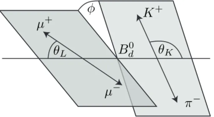
Three angular variables are used to describe the decay: the angle between theK+and the direction opposite to theB0d in theK∗ centre of mass frame (θK); the angle between the µ+ and the direction opposite to theB0din the di-muon centre of mass frame (θL); and the angle between the two decay planes formed by theKπand the di-muon systems in theB0d rest frame (φ). For B0dmesons the definitions are given with respect to the negatively charged particles. Figure1illustrates the angles used.
φ
Bd0 µ+
µ−
K+
π−
θL θK
Figure 1: An illustration of theB0
d →K∗µ+µ−decay showing the anglesθK,θLandφdefined in the text. Angles are computed in the rest frame of theK∗, di-muon system andB0
dmeson, respectively.
The angular differential decay rate for B0d → K∗µ+µ− is a function of q2, cosθK, cosθL and φ, and can be written in several different ways [13]. The form to express the differential decay amplitude as a function of the angular parameters uses coefficients that may be represented by the helicity or transversity amplitudes [14] and is written as2
1 dΓ/dq2
d4Γ
d cosθLd cosθKdφdq2 = 9 32π
"
3(1−FL)
4 sin2θK +FLcos2θK+ 1−FL
4 sin2θKcos 2θL
−FLcos2θKcos 2θL +S3sin2θKsin2θLcos 2φ +S4sin 2θKsin 2θLcosφ+S5sin 2θKsinθLcosφ +S6sin2θKcosθL+S7sin 2θKsinθLsinφ
+S8sin 2θKsin 2θLsinφ+S9sin2θKsin2θLsin 2φ
#
. (1)
HereFL is the fraction of longitudinally polarisedK∗’s and theSiare angular coefficients. These angular parameters are functions of the real and imaginary parts of the transversity amplitudes of B0d decays to K∗µ+µ−. The forward-backward asymmetry is given by AFB = 3S6/4. The Si parameters depend on hadronic form factors which have significant uncertainties at leading order. It is possible to reduce the theoretical uncertainty on the parameters extracted from data by transforming the Si using ratios constructed to cancel form factor uncertainties at leading order. These ratios are given by Refs [14,15]
2 This equation neglects possibleKπS-wave contributions. The effect of anS-wave contribution is considered following the method used by LHCb in [3].
as
P1 = 2S3
1−FL (2)
P2 = 2 3
AFB
1−FL (3)
P3 = − S9
1−FL (4)
Pi0=4,5,6,8 = Sj=4,5,7,8
pFL(1−FL). (5)
All of the parameters introduced, FL, Si andPi(0), vary with q2 and the data are analysed in q2 bins to obtain an average value for a given parameter in that bin. Measurements of these quantities can be used as inputs to global fits used to determine the values of Wilson coefficients and search for new physics.
3 The ATLAS detector, data, and Monte Carlo samples
The LHC collides bunches of protons in the vacuum of the beam pipe at the interaction point of the ATLAS experiment. The ATLAS detector, as described in Ref. [16], consists of an inner detector (ID), a calorimeter system and a muon spectrometer (MS). The ID consists of silicon pixel and strip detectors, with a straw tube tracker providing additional information for tracks passing through the central region of the detector3. The ID has a coverage of|η| <2.5, and is immersed in a 2T axial magnetic field generated using a superconducting solenoid. A calorimeter system, consisting of liquid argon and scintillating-tile sampling calorimeter sub-systems, surrounds the ID. The outermost part of the detector is the MS system, which employs several different detector technologies in order to provide muon identification and a muon trigger. A toroidal magnet system is embedded in the MS. The ID, calorimeter and MS systems have full azimuthal coverage.
The data analysed here were recorded in 2012 during the latter part of Run 1 of the LHC. The collision energy of the pp system was
√s = 8 TeV. After applying beam, detector and data-quality criteria, the data sample analysed comprises of an integrated luminosity of 20.3 fb−1. A number of Monte Carlo (MC) simulated event samples, generated using Pythia 8 [17] and EvtGen [18], with final state radiation simulated using PHOTOS [19] are used. Simulated events are passed through the Geant 4 [20,21] based ATLAS MC simulation programme and fed through the same reconstruction chain as data. These are studied in order to finalise event selection and explore potential backgrounds. The MC simulation includes modeling of multiple interactions perppbunch crossing in the LHC. The samples of MC generated events used are described further in Section5.
3ATLAS uses a right-handed coordinate system with its origin at the nominal interaction point (IP) in the centre of the detector and thez-axis along the beam pipe. The x-axis points from the IP to the centre of the LHC ring, and the y-axis points upward. Cylindrical coordinates(r,Φ)are used in the transverse plane,Φbeing the azimuthal angle around thez-axis. The pseudorapidity is defined in terms of the polar angleθasη=−ln tan(θ/2).
4 Event selection
Events satisfy a trigger that requires one, two, or more muons. Several trigger signatures constructed from the MS inputs are combined based on availability during the data taking period, prescale factor and efficiency for signal identification. Data are combined from 15 trigger chains where 21%, 89% or 5% of selected events pass at least one trigger with one, two, or at least three muons identified online in the MS, respectively. Of the events passing the trigger, 86% are required to have at least two muons identified at trigger level and the dominant single contribution comes from the requirement of one muon with a transverse momentumpT > 4 GeV and the other muon withpT > 6 GeV. This combination of triggers ensures that the analysis remains sensitive to events down to the kinematic threshold ofq2=4m2µ, where mµ is the muon mass. The effective average trigger efficiency for selected signal events corresponds to about 29%.
Muon tracks are formed offline by combining information from both the ID and MS [22]. Tracks are required to satisfy|η| < 2.5. Candidate muon (kaon and pion) tracks are required to satisfy pT > 3.5 (0.5) GeV. Pairs of oppositely charged muons are required to originate from a common vertex with a
χ2 <10.
CandidateK∗mesons are formed using pairs of oppositely charged kaon and pion candidates reconstructed from hits in the ID. Candidates are required to satisfypT(K∗) > 3.0 GeV. As the ATLAS detector does not have a dedicated charged particle identification system, candidates are reconstructed to satisfy both possibleKπmass hypotheses and the selection relies on the kinematics of the reconstructedK∗meson to determine which of the two tracks corresponds to the kaon. The invariantKπmass is required to lie in a window of twice the natural width around the nominal mass of 896 MeV, i.e. in the range[846,946]MeV.
The charge of the kaon candidate is used to assign the flavor of the reconstructedBcandidate.
B candidates are reconstructed from aK∗candidate and a pair of oppositely charged muons. The four- track vertex is fitted and required to satisfy χ2 < 2 to suppress background. A significant amount of combinatorial, B0d, B+, B0s andΛb background contamination remains at this stage. Combinatorial background is suppressed by requiring aB0dcandidate lifetime significanceτ/στ > 12.5, where the decay time uncertainty στ is calculated from the covariance matrices associated with the four-track vertex fit and with the primary vertex fit. Background from partially reconstructed decays exists below theB0dmass and feeds up into the signal region. This contribution is suppressed by requiring an asymmetric mass cut around the nominalBd0 mass, 5150 < mKπµµ < 5700 MeV. The high mass sideband is retained as the parameter values for the combinatoric background shapes are extracted from the fit to data described in Section5. To further suppress background it is required that the angle, Θ, defined between the vector from the primary vertex to the Bd0 candidate decay vertex and the Bd0 candidate momentum, satisfies cosΘ > 0.999. Resolution effects on cosθK, cosθL andφare found to have a negligible effect on the ATLASBs0→J/ψφanalysis [23] It is assumed to also be the case forB0d→K∗µ+µ−.
On average 12%, 2-10%, and 17% of events in the data, exclusive background, and signal MC have more than one candidate reconstructed, respectively. A two-step selection process is used for events containing more than one candidate. The majority, about 96%, of multiple candidates arise from degenerate four track combinations where the kaon and pion assignments are ambiguous. TheBd0candidate reconstructed with smallest value of |mKπ −mK∗|/σ(mKπ) is retained for analysis, where mKπ is the K∗ candidate mass,σ(mKπ)is the error on this quantity, andmK∗ is the world average value of theK∗ mass. For the remaining 4% of events, the candidate with the smallest value of theBvertexχ2is retained for subsequent analysis. This procedure results in an incorrect flavor tag (mistag) for some signal events. The mistag
probability of aBd0 (B0d) meson is denoted asω(ω) and is determined from MC simulated events to be 0.1088±0.0005(0.1086±0.0005). The mistag probability varies slightly withq2such that the difference ω−ωremains consistent with zero. Hence the average mistag ratehωiin a givenq2bin is used to account for this effect. If a candidate is mistagged then the values ofθK andφchange sign. Sign changes in these angles affect the overall sign of the terms multiplied by the coefficientsS4, S5 andS9 (similarly for the correspondingP(0)parameters) in Equation (1). The corollary is that mistagged events result in a dilution factor of(1−2hωi)for the affected coefficients.
The region q2 ∈ [0.98,1.1] GeV2 is vetoed to remove any potential contamination from the φ(1020) resonance. The remaining data with q2 ∈ [0.04,6.0] GeV2 are analysed in order to extract the signal parameters of interest. TwoK∗cccontrol sample regions are defined forBdecays toK∗J/ψandK∗ψ(2S), respectively asq2 ∈ [8,11]and[12,15]GeV2. The control samples are used to extract nuisance parameters of the signal probability density function (p.d.f.) from data as discussed in Section5.3.
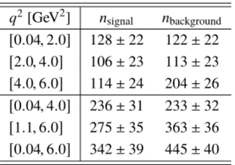
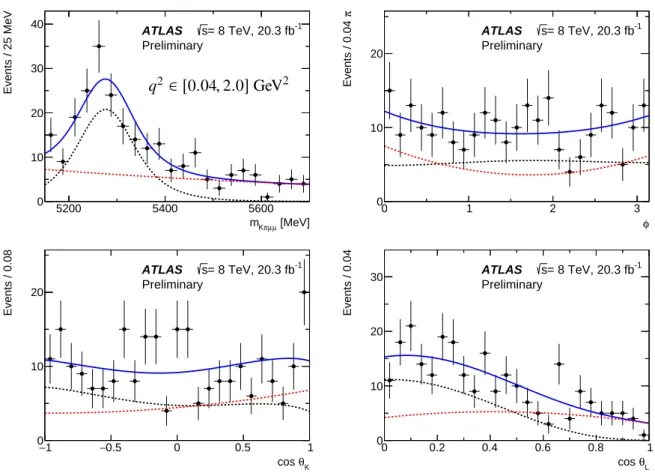
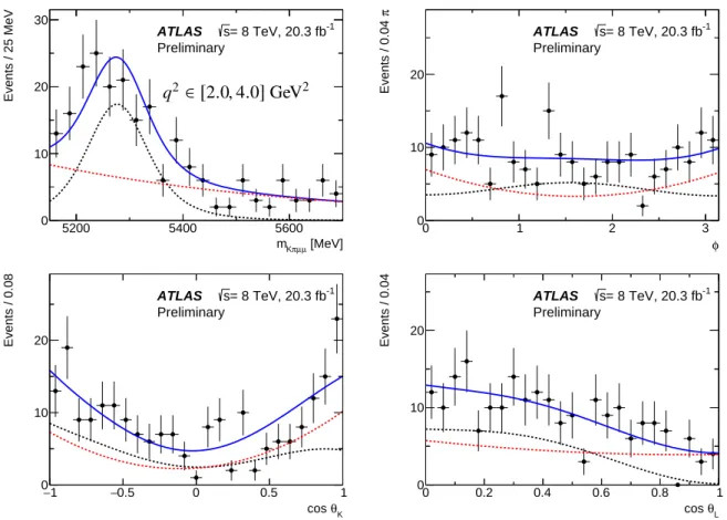
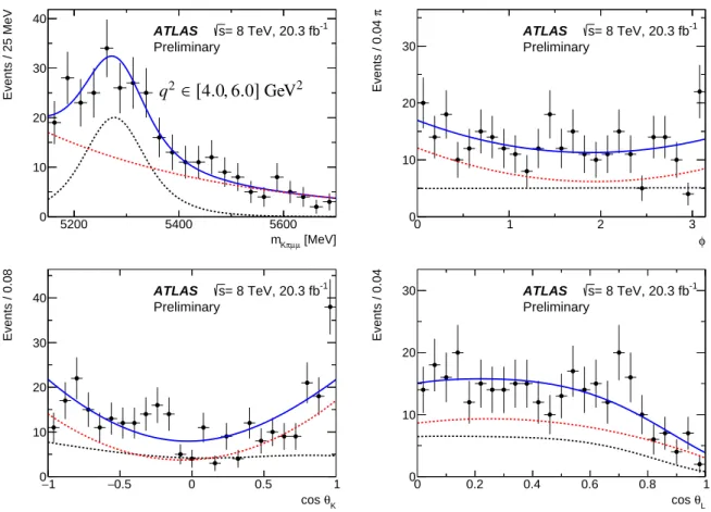
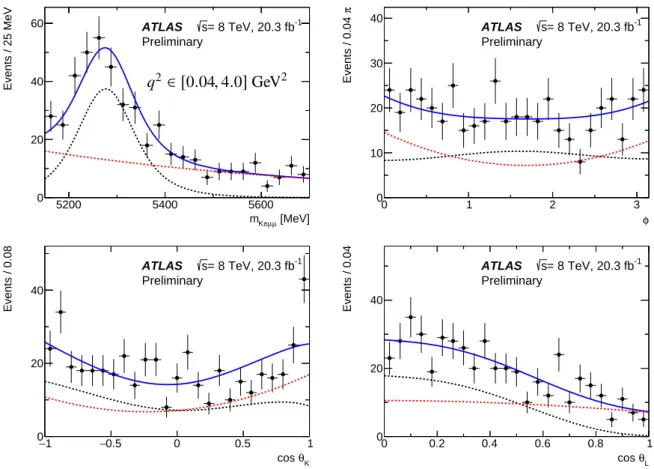
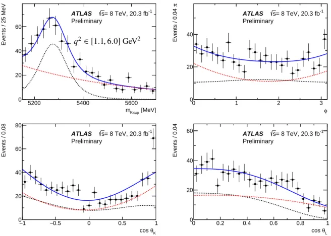
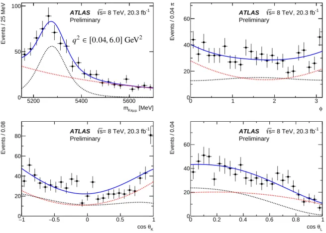
Forq2<6 GeV2the selected data sample consists of 787 events and is composed of signalB0d→K∗µ+µ− decay events as well as background that is dominated by a combinatorial component that does not peak inmKπµµ and does not exhibit resonant structure inq2. Other background contributions are considered when computing systematic uncertainties. Above 6 GeV2several backgrounds pass the selection imposed, including events coming from the low mass tail ofB →K∗J/ψ. ScalarKπcontributions are neglected in the nominal fit and considered only when addressing systematic uncertainties. The data are analysed in theq2bins[0.04,2.0],[2.0,4.0],[4.0,6.0],[0.04,4.0],[1.1,6.0],[0.04,6.0]GeV2, where the bin width is chosen to provide a sample of signal events sufficient to perform an angular analysis. The width is much larger than the resolution obtained from MC simulated signal events and than observed in data for Bd0 decays to K∗J/ψ and K∗ψ(2S) decays. The overlapping regions are analysed in order to facilitate comparison with other experiments and theory.
5 Maximum likelihood fit
Extended unbinned maximum likelihood fits of the angular distributions of the signal decay are performed on the data for eachq2 bin. The discriminating variables used in the fit aremKπµµ, the cosines of the helicity angles (cosθK and cosθL), andφ. The likelihoodL for a givenq2bin is
L = e−N n!
n
Ö
i=1
Õ
j
njPi j(mKπµµ,cosθK,cosθL, φ;bp,bθ), (6)
wheren is the total number of events, the sum runs over signal and background components, nj is the fitted yield for the jth component, N is the sum over nj, and Pi j is the p.d.f. evaluated for eventi and component j. For the nominal fit j = 2, as only one background component is considered. Thebp are parameters of interest (FL, Si) andbθ are nuisance parameters. The remainder of this section discusses the signal model (Section5.1), treatment of background (Section5.2), use ofK∗ccdecay regions in data (Section5.3), fitting procedure and validation (Section5.4).
5.1 Signal model
The signal mass distribution is modeled by a Gaussian distribution where the widthσof the Gaussian is scaled by the per-event uncertainty on theKπµµmass,σ(mKπµµ), i.e. the width is given byσ0σ(mKπµµ),
whereσ0is a unitless scale factor. The mean value of the B0d candidate mass (m0) andσ0of the signal Gaussian p.d.f. are determined from fits to the control sample regions of data as described in Section5.3.
Extraction of information using the angular distribution in Equation (1) places constraints on the minimum signal yield and the signal purity in order to avoid pathological fit behaviour. A significant fraction of fits to ensembles of simulated pseudo-experiments do not converge using the full distribution. This can be mitigated using trigonometric transformations to simplify the fit as terms in Equation (1) drop out when applying these ‘folding schemes’. Each transformation simplifies Equation (1) such that only three parameters are extracted from each of the four fits: FL, S3 and one of the other S parameters. The values and uncertainties of FL and S3 obtained from the four fits are consistent with each other and the results reported are those found to have the smallest systematic uncertainty. Following Ref. [3], the transformations listed below are used in order to extract the angular parameters reported here:
FL,S3,S4,P0
4:
φ→ −φ forφ < 0 φ→π−φ forθL > π θL →π−θL forθL > 2π 2,
(7)
FL,S3,S5,P0
5:
(φ→ −φ forφ < 0 θL →π−θL forθL > π
2, (8)
FL,S3,S7,P0
6:
φ→π−φ forφ > π φ→ −π−φ forφ < −2π
θL →π−θL forθL > π2 2,
(9)
FL,S3,S8,P0
8:
φ→π−φ forφ > π φ→ −π−φ forφ < −2π
θL →π−θL forθL > π2
θK →π−θK forθL > 2π 2.
(10)
On applying transformation (7), (8), (9), and (10), the angular variable ranges become cosθL ∈ [0,1],cosθK ∈ [−1,1]andφ∈ [0, π],
cosθL ∈ [0,1],cosθK ∈ [−1,1]andφ∈ [0, π], cosθL ∈ [0,1],cosθK ∈ [−1,1]andφ∈ [−π/2, π/2], cosθL ∈ [0,1],cosθK ∈ [−1,1]andφ∈ [−π/2, π/2],
(11) respectively. A consequence of using the folding schemes is thatS6 (AFB) and S9 can not be extracted from the data. The angular parameters of interest for these schemes denoted by bp in Equation (6) are (FL,S3,Si)wherei=4,5,6,8. These translate into(FL,P1,P0j), wherej=4,5,7,8, using Equation (5).
Three MC samples are used to study signal reconstruction, acceptance, mistag and the fit performance.
These assume either that the decays are flat in phase space, or follow the SM expectation taken from Ref. [24], where in the latter case separate samples are generated for B0d and B0d decays. The phase
space MC sample hasFL = 1/3 and the angular distributions are generated flat in cosθK, cosθL and φto study the effect of potential mistag and reconstruction differences between particle and antiparticle decays. The acceptance function is defined as the deviation from the generated distribution of cosθK, cosθL,φas a result of triggering, reconstruction and selection of events. This is described by 6th (2nd) order polynomial distributions for cosθK and cosθL (φ) and is assumed to factorise for each angular distribution, i.e. it is assumed thatε(cosθK,cosθL, φ)=ε(cosθK)ε(cosθL)ε(φ)is valid and a systematic uncertainty is assessed in order to account for this assumption. The acceptance function multiplies the angular distribution in the fit, i.e. neglecting the mass dependence the signal p.d.f. is
Pi j =ε(cosθK)ε(cosθL)ε(φ)g(cosθK,cosθL, φ), (12) where g(cosθK,cosθL, φ) is an angular differential decay rate resulting from one of the four folding schemes applied to Equation (1). The MC sample generated according to phase space is used to determine the nominal acceptance functions and the other samples are used for systematic uncertainty determination.
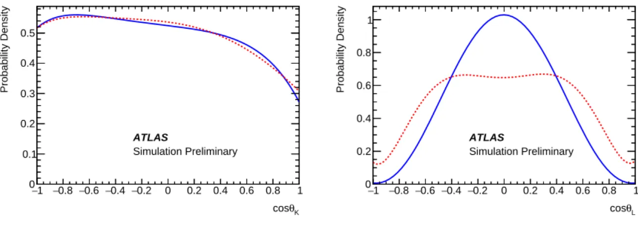
The acceptance function is evaluated using the nominal sample and for each of the transformed variables defined in Equations (7-10). These functions describe the bias in the angular event distributions resulting from the reconstruction and selection. Among the angular variables the cosθL distribution is the most affected by the acceptance. This is a result of the trigger thresholds and ability to reconstruct low momentum muon pairs that correspond to low values of q2. As q2 increases the acceptance effects become less severe. The cosθK distribution is also affected by the ability to reconstruct theKπsystem, however that effect shows no significant variation withq2. There is no significant acceptance effect for φ. Figure2shows the acceptance functions used for cosθK and cosθL for two differentq2ranges for the nominal angular distribution given in Equation (1).
θK
cos
−1 −0.8 −0.6 −0.4 −0.2 0 0.2 0.4 0.6 0.8 1
Probability Density
0 0.1 0.2 0.3 0.4 0.5
ATLAS
Simulation Preliminary
θL
cos
−1 −0.8 −0.6 −0.4 −0.2 0 0.2 0.4 0.6 0.8 1
Probability Density
0 0.2 0.4 0.6 0.8 1
ATLAS
Simulation Preliminary
Figure 2: The acceptance functions for (left) cosθKand (right) cosθLfor (solid)q2 ∈ [0.04,2.0]GeV2and (dashed) q2∈ [4.0,6.0]GeV2corresponding to the angular decay rate of Equation (1).
5.2 Background modes
The fit to data includes a combinatorial background component that does not peak in themKπµµ distri- bution. It is assumed that the background p.d.f. factorises into a product of one dimensional terms. The mass distribution of this component is described by an exponential function and second order Chebychev polynomials are used to model the cosθK, cosθLandφdistributions. The nuisance parameters describing these shapes are obtained from fits to the data independently for eachq2bin.
A total of seven inclusive and eleven exclusiveB0d,B0s,B+andΛbbackground samples are studied in order to identify contributions of interest to be included in the fit model, or to be considered when computing systematic uncertainties. The inclusive samples considered arebb→ µ+µ−X andcc → µ+µ−X decays and the relevant exclusive modes found to be of interest are discussed below. Bc decays are suppressed by excluding the q2 range containing the J/ψ and ψ(2S), and by charm meson vetoes discussed in Section7. The exclusive background decays considered for the signal mode areΛb → Λ(1520)µ+µ−, Λb → pK−µ+µ−, B+ → K(∗)+µ+µ−andB0s → φµ+µ−. These background contributions are accounted for as systematic uncertainties evaluated as described in Section7.
Two distinct background contributions not considered above are observed in the cosθK and cosθL distributions. They are not accounted for in the nominal fit to data, and are treated as systematic effects.
The peak in cosθK is found to be around 1.0 and appears to have two types of contribution. One of these arises from mis-reconstructedB+decays, such asB+→K+µµandB+→π+µµ. These decays can be reconstructed as signal if another track is combined with the hadron to form aK∗candidate in such a way that the event passes the reconstruction and selection. Events with a three track invariant mass, formed from one of the hadrons from theK∗candidate and the two muon candidates, that fall within a 50 MeV mass window relative to the nominalB+mass are removed from data when studying systematic uncertainties. This veto reduces the amount of data accumulated in cosθK around 1.0 and has a small effect on the signal efficiency. The second contribution comes from combinations of two charged tracks that pass the selection and are reconstructed as a K∗ candidate. These fakeK∗candidates accumulate around cosθKof 1.0 and are observed in theKπsidebands away from theK∗meson. They are distinct from the resonant structure of expected S, P and D-waveKπdecays resulting from aB0d → Kπµµtransition.
The origin of this source of background is not fully understood. The observed excess may arise from a statistical fluctuation, an unknown background process, or a combination of both. All events are retained for the nominal fit this region (cosθK > 0.9) is removed when evaluating systematic uncertainties.
The background that peaks in cosθL is studied using Monte Carlo simulated events for the decays D0 → Kπ, D+ → Kππ, Ds+ → K Kπ, and D∗s+ → K Kπ. Events with an intermediate charm meson, D0,D±(s)andD∗s+are found to pass the selection and are reconstructed in such a way that they accumulate around 0.7 in|cosθL|. These are removed from the data sample when studying systematic uncertainties by applying a veto window about the reconstructed charm meson mass. The optimal veto window is found to be 30 MeV wide using MC simulated events. A few percent of signal events are lost using these vetoes and a narrow hole in the cosθL acceptance distribution is created near|cosθL|of 0.7.
5.3 K∗c ccontrol sample fits
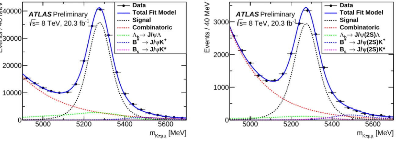
The mass distribution obtained in MC simulated samples forK∗ccdecays and the signal, in different bins ofq2, are found to be consistent with each other. Fits to the data are used to extract values ofm0andσ0 for B0d → K∗J/ψ andB0d → K∗ψ(2S)events that are used for the signal p.d.f. An extended unbinned maximum likelihood fit is performed to the twoK∗cc control sample regions allowing for 0, 1, 2 and 3 exclusive background components. The exclusive backgrounds included areΛb → Λcc, B+ → K+cc and Bs → K∗cc, respectively. The K∗cc p.d.f. has the same form as the signal model, combinatorial background is described by an exponential distribution, and double and triple Gaussian p.d.f.s determined from MC simulated events are used to describe the exclusive background contributions. The resulting distributions for the three exclusive background fits can be found in Figure3. The peak position and scale factor of the signal p.d.f. are not sensitive to the exclusive background model used. From these fits the statistical and systematic uncertainties on the values ofm0andσ0are extracted for theB0d component in
order to be used when theB0d →K∗µ+µ−fits are performed. From theJ/ψcontrol data it is determined that the signal Kπµµmass p.d.f. model nuisance parameters are m0 = (5276.6±0.3±0.4) MeV and σ0 = 1.210±0.004±0.002, where the uncertainties are statistical and systematic, respectively. The ψ(2S)sample yields compatible results albeit with larger uncertainties. These results are similar to those obtained from the MC simulated samples, and the numbers derived from theK∗J/ψdata are used for the signal region fits.
[MeV]
µ µ π
mK
5000 5200 5400 5600
Events / 40 MeV
0 10000 20000 30000
40000 ATLAS
= 8 TeV, 20.3 fb-1
s
Preliminary
Data Total Fit Model Signal Combinatoric
Λ ψ
→ J/
Λb
K+
ψ
→ J/
B+
ψK*
→ J/
Bs
[MeV]
µ µ π
mK
5000 5200 5400 5600
Events / 40 MeV
0 1000 2000 3000
ATLAS
= 8 TeV, 20.3 fb-1
s
Preliminary
Data Total Fit Model Signal Combinatoric
Λ ψ(2S)
→ J/
Λb
(2S)K+
ψ
→ J/
B+
(2S)K*
ψ
→ J/
Bs
Figure 3: Control sample fits to theKπµµinvariant mass distributions for the (left)K∗J/ψ and (right)K∗ψ(2S) regions. The data are shown as points and the total fit model as the solid lines. The dashed lines represent (black) signal, (red) combinatorial background, (green)Λb background, (blue) B+ background and (magenta)B0s background.
5.4 Fitting procedure and validation
A two-step fit process is performed for the different signal regions inq2. The first step is a fit to the Kπµ+µ−invariant mass distribution, using the event-by-event uncertainty on the reconstructed mass as a conditional variable. For this fit the parametersm0 andσ0 are fixed to the values obtained from fits to data control samples as described in Section5.3. A second step adds the (transformed) cosθK, cosθLand φvariables to the likelihood in order to extractFL and theSiparameters along with nuisance parameters related to the combinatorial background shapes. The nuisance parameters (m0,σ0, signal and background yields, and the exponential shape parameter for the background mass p.d.f.) are fixed to the nominal results obtained from the first step.
The fit procedure is validated using ensembles of simulated pseudo-experiments generated with theFL andS parameters corresponding to those obtained from the data. The purpose of these experiments is to measure the intrinsic fit bias resulting from the likelihood estimator used to extract signal parameters.
These ensembles are also used to validate that the uncertainty extracted from the fit is consistent with expectations. Ensembles of simulated pseudo-experiments are performed where signal MC is injected into samples of background events generated from the likelihood. The signal yield determined from the first step in the fit process is found to be unbiased. The angular parameters extracted from the nominal fits have biases ranging between 0.01 and 0.04, depending on the fit variation andq2bin. A similar procedure is used to estimate the effect of neglectingS-wave contamination in the data sample. Neglecting theS-wave component in the fit model results in a bias of between between 0.00 and 0.02 on the angular parameters.