Jens Karstens , Jonathan M. Bull , Ben J. Callow , Anna Lichtschlag , Mark Schmidt1 , Judith Elger1 , Bettina Schramm1 , and Matthias Haeckel1
1GEOMAR Helmholtz Centre for Ocean Research Kiel, Kiel, Germany,2Stockholm University and Bolin Centre for Climate Research, Stockholm, Sweden,3Ocean and Earth Science, University of Southampton, National Oceanography Centre, Southampton, UK,4National Oceanography Centre, University of Southampton Waterfront Campus,
Southampton, UK
Abstract
Marine sediments host large amounts of methane (CH4), which is a potent greenhouse gas.Quantitative estimates for methane release from marine sediments are scarce, and a poorly constrained temporal variability leads to large uncertainties in methane emission scenarios. Here, we use 2‐D and 3‐D seismic reflection, multibeam bathymetric, geochemical, and sedimentological data to (I) map and describe pockmarks in the Witch Ground Basin (central North Sea), (II) characterize associated sedimentological andfluid migration structures, and (III) analyze the related methane release. More than 1,500 pockmarks of two distinct morphological classes spread over an area of 225 km2. The two classes form independently from another and are corresponding to at least two different sources offluids. Class 1 pockmarks are large in size (>6 m deep, >250 m long, and >75 m wide), show active venting, and are located above verticalfluid conduits that hydraulically connect the seafloor with deep methane sources. Class 2 pockmarks, which comprise 99.5% of all pockmarks, are smaller (0.9–3.1 m deep, 26–140 m long, and 14–57 m wide) and are limited to the soft,fine‐grained sediments of the Witch Ground Formation and possibly sourced by compaction‐related dewatering. Buried pockmarks within the Witch Ground Formation document distinct phases of pockmark formation, likely triggered by external forces related to environmental changes after deglaciation. Thus, greenhouse gas emissions from pockmarkfields cannot be based on pockmark numbers and present‐dayfluxes but require an analysis of the pockmark forming processes through geological time.
Plain Language Summary
Marine sediments host large amounts of methane (CH4), which is a potent greenhouse gas. The amount of methane released into the atmosphere is, however, largely unknown making it difficult to implement this methane source in climate models. Here we use geophysical, geochemical, and sedimentological data to map the distribution offluid escape structures in the central North Sea. More than 1,500 pockmarks, which are circular to semicircular depressions of the seafloor, indicatefluidflow from the subsurface. There are two distinct morphological classes of pockmarks corresponding to at least two differentfluid sources. Class 1 pockmarks are large, show active venting, and are located above verticalfluid conduits in the subsurface, which feedfluids from deeper strata. Class 2 pockmarks, which comprise 99.5% of all pockmarks, are smaller and limited to the soft sediments directly below the seafloor. Older pockmarks in the subsurface document distinct phases of pockmark formation, likely triggered by external forces after the retreat of ice in the North Sea. The amount of methane released from natural geological sources based on pockmark numbers may be wrong as these do not take into account the origin and composition of releasedfluids.1. Introduction
Earth's climate is highly sensitive to the release of potent greenhouse gases such as methane (CH4) into to atmosphere. Methane has been released during climatic changes including the steepest known natural tem- perature increase on Earth at the Paleocene‐Eocene Thermal Maximum around 55.5 Ma ago (Dickens, 2011;
Svensen et al., 2004) but also during and after the Younger Dryas‐Preboreal abrupt warming event at the beginning of the Holocene (about 11,600 cal. years BP; Petrenko et al., 2017). However, current and future methane emissions remain poorly constrained and bottom up as well as top down approaches for the quan- tification of methane emissions have large uncertainties (Dean et al., 2018; Petrenko et al., 2017). The global methane emission from natural geological sources shows a wide range in estimates (33–75 Tg CH4per year;
©2019. American Geophysical Union.
All Rights Reserved.
Key Points:
• Marine geophysical data document
>1,500 pockmarks of two morphological classes in the Witch Ground Basin, central North Sea
• Class 1 pockmarks are continuously active and supplied through seismic pipe structures by deeply sourced methane
• Class 2 pockmarks form at specific stratigraphic horizons suggesting intermittent venting triggered by pressure and temperature changes
Correspondence to:
C. Böttner, cboettner@geomar.de
Citation:
Böttner, C., Berndt, C., Reinardy, B. T.
I., Geersen, J., Karstens, J., Bull, J. M., et al. (2019). Pockmarks in the Witch Ground Basin, central North Sea.
Geochemistry, Geophysics, Geosystems, 20, 1698–1719. https://doi.org/10.1029/
2018GC008068
Received 7 NOV 2018 Accepted 11 MAR 2019
Accepted article online 14 MAR 2019 Published online 1 APR 2019
Ciais et al., 2013; Etiope et al., 2008), which highlights the large uncertainties involved in attributing and quantifying methane emissions.
Marine sediments host large amounts of methane in the form of free gas, hydrates, or dissolved in porewater.
There is evidence for direct contribution of methane from shallow marine sediments to the atmospheric methane budget and hence to climate change (Etiope et al., 2008; Judd et al., 2002). Methane formed in mar- ine sediments may either be biogenic (derived from microbial degradation of organic matter) or thermogenic (generated in deep hydrocarbon reservoirs by thermal cracking of kerogens; Whiticar, 2000). The carbon and hydrogen isotope signatures and the relative proportions of methane and more mature hydrocarbons (e.g., ethane, propane, butane) can help distinguish between the two sources (Whiticar, 2000). Methane from both onshore and offshore microseep and macroseep contributes to the atmospheric methane budget and can be supplied by geothermal, volcanic, or sedimentary sources (Dean et al., 2018; Etiope et al., 2008; Saunois et al., 2016). In the marine environment, methane may accumulate in the subsurface, when gas pressure exceeds the ambient hydrostatic pressure and the methane forms gas bubbles, which may be released by diffusion or episodic ebullition (Boudreau et al., 2005; Krämer et al., 2017; Maeck et al., 2013). However, the global sig- nificance of marine methane sources and their impact on the global methane budget remains poorly con- strained (Ciais et al., 2013; Etiope et al., 2008; Petrenko et al., 2017).
One manifestation of focusedfluid migration at the seafloor are circular to semicircular depressions known as pockmarks, which may form in response to venting offluids from the seafloor Hovland & Judd, 1988;
King & McLean, 1970). Pockmarks may be meters to hundreds of meters in diameter, meters to tens of meters in depth and affect the local environment, morphodynamics, biochemistry, and ecology (Berndt, 2005; Dando et al., 1991; Judd & Hovland, 2007; Niemann et al., 2005; Wegener et al., 2008). Increasing high‐resolution bathymetric data coverage reveals the wide abundance of pockmarks at the seafloor in var- ious structural and geologic settings (e.g., Brothers et al., 2012; Gafeira et al., 2018; Hovland et al., 2002).
Understanding the processes that control the formation and activity of pockmarks is crucial to estimate the contribution of methane from natural geological sources to the atmospheric methane budget and its impact on climate change.
Pockmarks often form on top of focusedfluid conduits, which manifest in seismic data as seismic chimneys or pipes and are characterized by circular‐shaped amplitude anomalies with dimmed reflections and bright spots at different depth levels (Andresen, 2012; Cartwright et al., 2007; Karstens & Berndt, 2015; Løseth et al., 2009). The terms seismic chimneys or pipes and pockmarks are attributed to the localized release of over- pressure in the subsurface through hydraulic connection of deeper strata with the seafloor (Cole et al., 2000; Hustoft et al., 2009). Pockmarks that formed above pipe and chimney structures are observed globally, for example, at the Vestnesa Ridge NW off Svalbard (Hustoft et al., 2009; Plaza‐Faverola et al., 2017), in the Nyegga pockmark field on the continental Norwegian margin (Karstens et al., 2018), offshore Nigeria (Løseth et al., 2011), in the Western Nile Deep Sea Fan (Moss et al., 2012), and in the Lower Congo Basin (Gay et al., 2007).
The aim of this study is to analyze pockmark‐forming processes in the Witch Ground Basin, central North Sea (Figure 1). Wefirst map the abundant pockmarks and characterize them based on their morphology and subsurface preconditions. Second, we determine the source offluids that contribute to pockmark forma- tion in the Witch Ground Basin and investigate the interrelation offluidflow and depositional processes dur- ing their formation. This includes determining if there are different sources offluids, if they are located at different depths, and if they provide different types offluids. Subsequently we constrain the timing and the recurrence rate of pockmark formation in the Witch Ground Basin.
2. Regional Setting
2.1. Pockmarks in the Central North Sea
The North Sea is affected by focusedflow of hydrocarbons from deep thermogenic sources, strongly mixed with microbially formed shallow methane (Chand et al., 2017; Karstens & Berndt, 2015). Three decades of extensive surveying and seafloor mapping in the Witch Ground Basin has revealed abundant“normal” pockmarks and multiple“unusually large”pockmarks. These pockmarks indicate significantflow offluids from shallow marine sediments (Gafeira et al., 2018; Hovland & Sommerville, 1985; Judd et al., 1994;
Pfannkuche, 2005). The term normal pockmark describes pockmarks that are more than 5 m in diameter and found in isolation where free gas pockets in the subsurface degas cyclically (Hovland et al., 2010).
The so‐called unusually large pockmarks are complexes of pockmarks that are >100 m in diameter and
>10 m deep. They are located in UK block 15/25 and include the Scanner, Scotia, Challenger, and Alkor pockmark complexes, of which Scanner and Scotia comprise two large adjacent pockmarks (Gafeira &
Long, 2015; Judd et al., 1994). Ongoing seepage is interpreted from repeated water column imaging (multi- ple cruises from 1983–2005; Dando et al., 1991; Judd et al., 1994; Judd & Hovland, 2007; Gafeira & Long, 2015) and visual evidence of emerging bubbles (Remotely operated vehicles, 1985, 2004; submarine Jago, 1990; Gafeira & Long, 2015). Methane derived‐authigenic carbonates (MDACs; Dando et al., 1991;
Hovland & Irwin, 1989), bacterial mats (Dando et al., 1991; Pfannkuche, 2005), and seep‐associated fauna (Austen et al., 1993; Dando et al., 1991) indicate long‐lasting seepage from these unusually large pockmarks.
The normal pockmarks formed in the soft,fine‐grained sediments of the Witch Ground Formation and have been identified across the Witch Ground Basin (Gafeira et al., 2018; Judd et al., 1994; Long, 1992; Sejrup et al., 1994; Stoker & Long, 1984). Their morphometry deviates strongly from the large pockmarks, as they are mostly less than 3 m deep and 20–40 m wide. The density ranges from less than 5 pockmarks per square kilometer at the outer parts of the Witch Ground Basin, to almost 30 pockmarks per square kilometer at the center, where water depth exceeds 150 m (Gafeira et al., 2018). There is seismic evidence that these normal pockmarks occur in tiers at distinct stratigraphic layers and not only at the surface (Figure 4a; Stoker & Long, 1984). Previous studies indicate that the density of pockmarks per tier increases with decreasing burial depth (Long, 1992). The lack of evidence for seepage from repeated water column imaging suggests intermittent activity of these normal pockmarks assuming they are formed by seepage (Gafeira & Long, 2015; Judd et al., 1994).
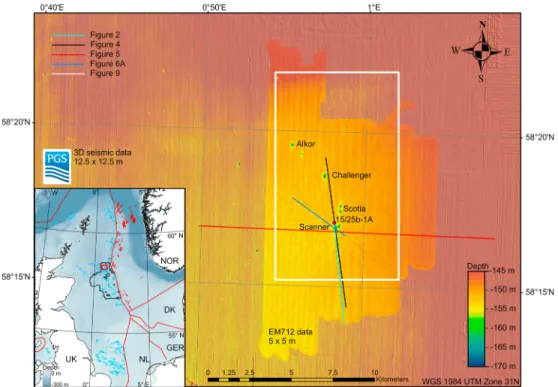
Figure 1.Bathymetric grid of the Witch Ground Basin, central North Sea. The shown bathymetry is a compilation of 3‐D reflection seismic data (converted with 1,500 m/s constant velocity, 12.5 × 12.5 m lateral resolution) and EM712 (5 × 5 m lateral resolution). Locations for additionalfigures are indicated, turquoise line = Figure 2, black line = Figure 4c, red line = Figure 5b, blue line = Figure 6a, white line = Figures 9a–9c. The inset shows the location of the study area (red box) within the North Sea (EMODnet bathymetric map projected in UTM zone 31, WGS84). The black line outlines the PGS“CNS MegaSurveyPlus.”Colored polygons show Norwegian (red, Norwegian petroleum directorate open data) and UK (blue, oil and gas authority open data) hydrocarbonfields.
2.2. Stratigraphy of the Witch Ground Basin
The Witch Ground Basin is located above the Witch Ground Graben, which is a major structural feature that developed between Triassic and Early Cretaceous times (Andrews et al., 1990). During the Late Jurassic and Early Cretaceous, the basin was a major sediment depo‐center (Andrews et al., 1990). Clays with interbeds of sandstone and limestone dominate the Paleogene and Neogene sequences (Figure 2). The Witch Ground Basin was again a deposition center during the Quaternary (~600 m of sediment). The shallow sediments and especially the Early Pleistocene sediments of the Aberdeen Ground Formation show evidence for sub- glacial, glaciomarine, and marine conditions (Buckley, 2012, 2016; Rea et al., 2018; Reinardy et al., 2017;
Rose et al., 2016; Sejrup et al., 1987; Stoker & Bent, 1987). On seismic reflection sections, the Aberdeen Ground Formation is characterized by laterally continuous, high amplitude reflections (Ottesen et al., 2014). The top of the Aberdeen Ground Formation is defined by a regional glacial unconformity and dissec- tion by a large number of tunnel valleys. The age of this unconformity is poorly constrained but it is thought to correspond to the advance of grounded ice into the North Sea Basin during the Mid Pleistocene Transition (~1.2–0.5 Ma; further referred to as R4; Reinardy et al., 2017). The tunnel valleys that dissect the unconfor- mity are part of the overlying Ling Bank Formation. This unit comprises a multitude of glacial tunnel valleys with different phases of erosion and deposition with poorly constrained ages. Comparison with tunnel val- leys of onshore mainland Europe where the valley infill and associated facies have been dated to the Holsteinian interglacial corresponding toMarineIsotopeStage (MIS) 11 gives a minimum age for formation of the stratigraphically lowest set of tunnel valleys in the North Sea during the Elsterian glaciation (MIS 12;
Stewart & Lonergan, 2011). The upper Mid to Late Pleistocene sedimentary succession consists of the Coal Pit, Swatchway, and Witch Ground Formations (Figure 2). The Coal Pit Formation comprises glacial till with Figure 2.(a) Stratigraphic and lithological summary of well 15/25b‐1A, located 400 m northwest of the western Scanner pockmark (modified after Judd et al., 1994). (b)6‐km‐long representative seismic profile from conventional 3‐D seismic data from north‐northwest to south‐southeast. The seismic profile shows major stratigraphic units lower Aberdeen Ground Formation (S1.1), R4 reflector, upper Aberdeen Ground Formation (S1.2), Ling Bank Formation (S2), Coal Pit Formation (S3), last glacial maximum deposits (LGM, S4) and the Witch Ground Formation (S5). The image shows distance along profile on thexaxis and two‐way traveltime (TWT) on theyaxis. 1.4 s TWT correspond to a minimum depth of 1,050 m (at 1,500 m/s seismic velocity). The location of the profile is given in Figure 1.
hard, dark gray to brownish‐gray, muddy, pebbly sands or sandy muds deposited between MIS 3 and 6 (Andrews et al., 1990; Graham et al., 2010; Stoker et al., 2011). The Swatchway Formation comprises silty sandy clays with rare pebbles; possibly proximal glaciomarine sediments deposited during MIS2–3. The uppermostfinely laminated, glaciomarine sediments of the Witch Ground Formation were deposited during MIS 1–2 (Stoker et al., 2011). The upper part of the Witch Ground Formation comprises Holocene age sedi- ments, which were reworked during the past 8 ka, when sedimentation decreased or ceased to virtually no sediment input into the Witch Ground Basin (Erlenkeuser, 1979; Johnson & Elkins, 1979).
3. Methods
3.1. Seismic Reflection Data
We used an extensive 3‐D industry seismic data set (“CNS MegaSurveyPlus”provided by PGS) that covers
>22,000 km2of the central to northern North Sea down to 1.5 s two‐way traveltime (TWT, Figure 1). The 3‐D pre‐stack time‐migrated seismic amplitude data (full fold stack) extends approximately 200 km from north to south and 140 km from east to west. The vertical resolution is approximately 20 m with an inline and crossline spacing of 12.5 m. Data sets like this have proven to be useful to identifyfluidflow systems, including their geometry, permeability barriers, andfluid accumulations, as they manifest in seismic data as amplitude anomalies (Karstens & Berndt, 2015).
We have used seismic attributes to enhance seismic interpretation including the Kingdom Suite Symmetry attribute, which is a post‐stack, post migration structural feature detection tool (e.g., fracture detection) based on a 3‐D log‐Gaborfilter array (Yu et al., 2015). This attribute is highly sensitive to seismic amplitude variations and therefore correlates with curvatures and discontinuities associated with geological structures, for example, faults, fractures, and discontinuous events (Böttner et al., 2018). In addition, we use the root‐ mean‐square (RMS) amplitude calculated over a time window of ±50 ms around the picked horizon (see horizon in Figure 2b, dashed blue line). RMS amplitude is a post‐stack attribute that highlights areas with direct hydrocarbon indicators such as bright spots by calculating the root of squared amplitudes divided by the number of samples per specified time window.
In addition, we acquired high‐resolution 2‐D seismic reflection data during research cruise MSM63 in April/May 2017 onboard RV Maria S. Merian (Figure 1, red/black lines). The aim of the seismic survey was to increase seismic resolution, map thefluidflow systems, and image the presumed subsurface fracture networks. The seismic profiles were acquired with a two‐105/105‐in3‐GI‐Gun‐array shot at 210 bar every 5 s and a 150 m‐long streamer with 96 channels and 1.5625 m channel spacing. The resulting shot point distance is approximately 8.75–12.5 m at 3.5–5 kn ship speed. The frequency range of the two‐GI‐Gun‐array is 15–
500 Hz. The processing included geometry and delay corrections, static corrections, binning to 1.5625 m and band‐passfiltering with corner frequencies of 25, 45, 420, and 500 Hz. Furthermore, a normal‐move‐
out‐correction (with a constant velocity of 1488 m/s calculated from CTD measurements) was applied and the data were stacked and then migrated using a 2‐D Stolt algorithm (1,500 m/s constant velocity model).
The vertical resolution of the processed data is approximately 6–7 m near the seafloor.
3.2. Seismostratigraphic Framework
Fluidflow in this area strongly depends on the local and regional stratigraphy and subsequent sediment properties. We have compiled a stratigraphic framework with seismic reflection data, industry well 15/25b‐1A (Figure 2a), British Geological Survey boreholes BH77/2, BH86/26, BH04/01 (Figure 1), and information from literature (Graham et al., 2010; Holmes, 1977; Judd et al., 1994; Long et al., 1986; Sejrup et al., 2014; Reinardy et al., 2017). We are able to tie most seismostratigraphic units within our stratigraphic framework to previously published lithostratigraphic units (Figure 2). Formation names and their ages uti- lize the North Sea Quaternary lithostratigraphic framework (Stoker et al., 2011). The seismostratigraphic unit S1.1 corresponds to the lower Aberdeen Ground Formation (MIS 100–21); S1.2 to the upper Aberdeen Ground Formation (MIS 21–13); S2 inside the tunnel valleys to the Ling Bank Formation (MIS 12–10), which is unconformably overlain by regional glacigenic sediments deposited during Mid Pleistocene (MIS 6; Reinardy et al., 2017); S3 to the Coal Pit Formation (MIS 6–3); S4 to the upper Swatchway or lower Witch Ground Formation (MIS 3–2); and S5 to the Witch Ground Formation (MIS 2–1). However, previous interpretations and stratigraphic units likely include sediments of different
provenance due to lower resolution data. Possible reworking and disturbance byfluvial, glacial, and marine processes further complicate the interpretation of lithostratigraphic units in this part of the Witch Ground Basin (Sejrup et al., 2014).
3.3. Hydroacoustic Data
The shallow seismic stratigraphy was imaged by subbottom profiler (SBP) data acquired during cruise MSM63 (Figure 1, blue/black line) using Parasound P70 with 4 kHz as the secondary low frequency to obtain seismic images of the upper 100 m below the seafloor with very high vertical resolution (<15 cm). We applied a frequencyfilter (low cut 2 kHz, high cut 6 kHz, 2 iterations) and calculated the envelope within the seismic interpretation software IHS Kingdom. In addition, further SBP data were acquired during cruise JC152 (onboard RV James Cook in August 2017) using a Chirp. The Chirp SBP produces a sweep, which lasts 0.035 s; the normalized zero‐phase Klauder wavelet from the autocorrelation of the sweep shows a temporal length of 0.00075 s, allowing further processing. The bandwidth ranges from 2.8 to 6 kHz, with a central fre- quency of 4.4 kHz. The combination of both systems and the subsequent integrated data set enables a detailed analysis of the shallow sedimentary succession up to 50 m below the seafloor. Both systems are further referred to as echosounder.
Bathymetric data were acquired with the EM712 system mounted to the hull of RV Maria S. Merian (Figure 1). The survey was designed to provide high‐resolution bathymetry with 5 × 5 m resolution. We pro- cessed the data using MB Systems software (Caress & Chayes, 2017) and included statistical evaluation of soundings that increased the signal‐to‐noise ratio. The sound velocity profile for multibeam processing was measured at the beginning and at the end of the cruise.
3.4. Semiautomated Picking of Pockmarks
To delineate pockmarks within the MSM63 bathymetric data we used a workflow that combines multiple ArcGIS geoprocessing tools (also compare Gafeira et al., 2012, Gafeira et al., 2018). In afirst step, all depres- sions shallower than 18 m werefilled with the“fill”tool. Subsequently the original grid was subtracted from thefilled grid and all areas that have changed vertically by 0.5 m or more were classified. The“raster to poly- gon”tool was then used to draw polygons around the classified areas. Afterward, the areas were calculated for all polygons and those comprising <500 m2were deleted. This removed a vast quantity of polygons from the outer regions of single swath transects where the noise level within the multibeam data increased. After this step, the polygon data set was manually inspected and all polygons that did not encircle pockmarks were manually removed. This manual editing step was necessary due to the presence of some large (>500 m2) noisy regions within the multibeam data. Subsequently all empty areas within individual polygons were removed with the“Eliminate Polygon Part”tool. This removed the bathymetric noise within single pock- marks. The outlines of the polygons were then smoothed with the“smooth polygon”tool using a polynomial approximation with exponential kernel algorithm and a 100 m smoothing tolerance. Finally, the depth, the orientation and length of the longest and shortest axis, the perimeter, and the distance to the closest neigh- bor pockmarks were calculated for each pockmark defined by a polygon.
3.5. Sediment Sampling
Shallow sediment samples were taken at the southwestern edge of the western Scanner pockmark during R/V Poseidon cruise POS518 (Leg2) using a 6 m‐long gravity corer (Linke & Haeckel, 2018). At the core loca- tion, the shallow sedimentary succession thins out, thus allowing the sampling of the underlying strati- graphic layers. The cores were split in 1 m segments of archive and working halves.
The working halves were sampled for physical sediment properties, element composition of solid phase, and chemical composition of porewater. Porewater was extracted from sediment in 30 cm intervals using Rhizons (0.2μm, Rhizosphere Research Products, e.g., Seeberg‐Elverfeldt et al., 2005). Sulfate and chloride concentrations of sampled porewater were determined by Ion Chromatography equipped with a conductiv- ity sensor (Eco IC, Metrohm; Metrosep A Supp5–100/4.0). Analytical precision is ~1% (1σ) measured by repeated analysis of IAPSO (International Association for the Physical Sciences of the Oceans). Total organic carbon content (Corg), C/N‐ratio, and inorganic carbon content (CaCO3) were determined by combustion of sediment samples in a EURO Element Analyzer (C/N/S configuration), prior and after removal of inorganic carbon with 1 M HCl. The analytical data are given in percent of the total weight of dried sediment with an accuracy of 3%. Calculated C/N‐ratios are given in atom‐ratios. Dissolved methane concentrations were
determined by headspace sampling according to Sommer et al. (2009). Three cubic centimeters of sediment are transferred into a 22 ml head space vial and closed with a crimped rubber septum after adding 6 ml of saturated sodium chloride solution. Equilibrated headspace gases were analyzed by injecting 100μl of head- space gas into a Shimadzu gas chromatograph (GC‐2014) equipped with a packed Haysep‐Q (80/100, 8 ft) column and aflame ionization detector. Analytical data are given with 2% (1σ) accuracy. Sediment porosity was determined by weight difference due to loss of water from ~5 cm3wet sediment samples during freeze‐ drying.
The archive halves were used to measure the relative abundance of the elements Ca, Fe, S, Rb, Zr, and Cl at the British Ocean Sediment Core Research Facility (Southampton, UK) using the ITRAX core‐scanning X‐rayfluorescence system (Cox Analytical; Croudace et al., 2006). This was done in 1‐mm intervals using a molybdenum X‐ray tube at 30 s measurements time, 30 kV, and 40 mA. Element abundances are presented as total counts normalized to counts per second and a running average of 1 cm was applied to the results.
Physical properties (resistivity, magnetic susceptibility, and density) of the sediments were measured on the archive halves using the GEOTEK multisensor core logger at 1 cm intervals.
4. Results
4.1. Seafloor Morphology
High‐resolution bathymetric data reveal abundant depressions of the seafloor in various shapes and sizes in the Witch Ground Basin. These abundant depressions occur in water depths between 120 and 180 m over an area 225 km2and we interpret them as pockmarks (Figure 3). Where pockmarks are absent, the seafloor is characterized by linear and curvilinear depressions, which we interpret as iceberg plow marks (Figure 3a).
We identified 1679 individual pockmarks within our bathymetric grid. The derived morphological para- meters are summarized in Table 1.
The pockmarks are usually elongated in one direction with a long axis orientation in NNE to SSW direction (Figure 3b). The predominant long axis orientations do not align with the orientation of the sail line (20° off- set) and are therefore no acquisition artifacts. Based on their depths, widths, and lengths, we separate the pockmarks into two classes: Class 1 pockmarks (n= 9) include the Scanner, Scotia, Challenger, and Alkor pockmark complexes, which are >6 m deep, >75 m wide, and >250 m long (Figure 3a); Class 2 pockmarks represent the vast majority of pockmarks with depths between 0.9 and 3.1 m, width between 14 and 57 m and length between 26 and 140 m (n= 1670, Table 1).
4.2. Seismic Stratigraphy
A 3‐D seismic profile shows the major seismostratigraphic units and is centered above the western part of the Scanner Pockmark (Figure 4c). Following the local seismostratigraphic framework, unit S1.1 shows laterally highly coherent andfinely laminated seismic reflections, with an upper boundary defined by a distinct unconformity (R4), which is characterized by a zone of chaotic incoherent reflections (Figures 2b, 4c, and 5b). Unit S1.2 shows high lateral continuity of seismic reflections cut by numerous glacial tunnel valleys indicating different phases of erosion and deposition. The overlying unit S2 is discordant (erosional surface) and of chaotic to transparent seismic facies (Figures 4b and 5b). S2 varies in thickness between 0.015 and 0.050 s TWT corresponding to 10–40 m, and shows high amplitude patches (bright spots) with polarity rever- sals at stratigraphic highs in between adjacent tunnel valleys (Figures 4b and 5b), indicating the presence of free gas in pore space (Løseth et al., 2009). In the 3‐D seismic data, unit S3 is characterized by a chaotic to transparent seismic facies at the bottom and laterally continuous, low reflective seismic reflections at the top (Figure 4c). Based on the echosounder and 2‐D seismic data we subdivide this unit into two subunits (S3.1 and S3.2, see Figures 4a and 4b). S3.2 shows a transparent to chaotic seismic facies at the bottom and a transition to laminated seismic reflections at the top (Figures 4a and 4b and 5). Thisfine lamination of seismic reflections is also visible below 0.25 s TWT within the echosounder data (Figure 4a).
Figure 5 shows in further detail that unit S4 is discordant to S3.2 and characterized by a transparent to chao- tic seismic facies and internal alternating dipping reflections separated by a distinct boundary (Figure 5a).
Based on the echosounder data and the smeared boundary with high amplitude reflections (Figure 5a), we separate unit S4 into subunits S4.1 and S4.2. S4.1 varies in thickness (up to 0.033 s TWT corresponding to 25 m at 1,500 m/s) and thins out eastward toward the Scanner pockmark (Figure 5a). Unit S5 shows
well‐stratified and laterally continuous seismic reflections, which overly the corrugated surfaces of S4.1 and S4.2 (Figure 5). Based on the echosounder and 2‐D seismic data, we subdivide S5 into two subunits (S5.1 and S5.2, Figures 4a and 4b), which will be described in detail below.
4.3. Shallow Sedimentary Succession and Water Column Imaging
The high‐resolution echosounder data image the very shallow sedimentary succession, including units S4 and S5 (Figure 6a). S4.1 is characterized by a chaotic to transparent facies with a highly corrugated surface and internal reflections that show alternating dipping directions. S4.1 is mostly present below 0.23 s TWT and surficially exposed at the center of the western Scanner pockmark (see also inset Figure 4a).
Table 1
Statistical Analyses of Geomorphological Parameters Derived From 1,679 Individual Pockmarks in our Survey Area
Parameter Min. Max. Mean Std.
Percentage in range
Area [m2] 503 660,991 7,039 48,998 99% in 503–56,038 m2
Length [m] 13 1,106 83 57 93% in 26–140 m
Width [m] 6 464 36 22 92% in 14–57 m
Max. depth [m] 0.55 17.77 2.0 1.1 87% in 0.9–3.1 m
Perimeter [m] 32 2439 196 128 94% in 68–324 m
Neighboring distance [m] 0 583 102 60 69% in 42–162 m
Water depth [m] 144 155 151 2 61% in 149–153 m
Note. Minimum, maximum, mean, standard deviation, and percentage within range of area, length (aaxis), width (b axis), maximum depth (from threshold), perimeter, neighboring distance, and water depth at center point of respective pockmark.
Figure 3.(a) Detailed bathymetric map with a compilation of high‐resolution multibeam bathymetry (5 × 5 m lateral and up to 10 cm vertical resolution) and depth converted 3‐D seismic seafloor horizon in greyscale slope shader (12.5 × 12.5 lateral and ~20 m vertical resolution, converted with constant seismic velocity 1,500 m/s). The semiautomatically picked pockmarks are outlined by black polygons. White arrows highlight class 1 pockmarks outside of the high‐resolution bathymetry. (b) Zoom of Scanner, Scotia, and Challenger pockmarks and numerous class 2 pockmarks. Semiautomatedly picked pockmarks are outlined by black polygons. (c) Rose‐diagram of pockmark orientation (orientation ofaaxis).
S5.1 lies between 0.212 and 0.230 s TWT and consists of laterally continuous, very well laminated strata and high amplitude response (corresponding to dark colors in the echosounder profile). S5.1 also holds v‐shaped amplitude anomalies at specific stratigraphic horizons terminating at two major stratigraphic boundaries (red boxes I and II in Figure 6a). On top, S5.2 (0.208–0.215 s TWT) shows lower amplitudes, but a well laminated and lateral coherent stratigraphy. This unit reveals as well v‐shaped amplitude anomalies marked with red boxes III and IV. The v‐shaped amplitude anomalies show very high amplitudes (black arrows in Figure 6a) at their center. They all terminate at the same stratigraphic horizon. Both S5.1 and S5.2 show local vertical amplitude discontinuities, possibly indicating fractures in the subsurface (Figure 6a). The topmost part of unit S5.2 between the seafloor at 0.205–0.207 s TWT is characterized by a high amplitude Figure 4.Combination of (a) echosounder data, (b) 2‐D seismic reflection data, and (c) 3‐D seismic reflection data extending from northwest to southeast across the Scanner pockmark showing interpreted horizons, interpreted seismic units S1 to S5 and unconformity R4. The dashed box in (c) shows location of (b), dashed box in (b) shows location of (a) and dashed box in (a) shows location of zoomed section in the right corner. Horizons are as follows: red line = R4; dashed blue line = top S1.2; pink line = top S2; dashed slate blue line = top S3.2; bright blue line = top S4.1; blue line = top S5.1;
yellow line = seafloor (SF). Vertical red bar in (c) shows the location of industry well 15/25b‐1A. The location of the profile is given in Figure 1. TWT = two‐way traveltime.
chaotic seismic facies. Here, the class 2 pockmarks crop out at the seafloor and the unit comprises another set of v‐shaped amplitude anomalies, which coincide with the pockmarks at the seafloor. This indicates that the v‐shaped amplitude anomalies in the subsurface most probably correspond to previous phases of pockmark formation (further referred to as paleo‐pockmarks, red boxes I–IV). If single seep sites would have been active over a long time, this activity would lead to stacked pockmarks (Andresen & Huuse, 2011). However, paleo‐pockmarks in the subsurface do not coincide with class 2 pockmarks at the seafloor. The echosounder data allow to determine the thickness of the sediment in unit S5.2, in which the vast majority of pockmarks and paleo‐pockmarks are located (Figures 6a and 7a and 7d).
We observed no venting from class 2 pockmarks during MSM63 (April/May 2017). However, our backscatter images show high values for class 2 pockmarks around their center and their rim, of which the latter is most likely related to slope effects (Figure 6d). Active venting was limited to the class 1 pockmarks Scanner, Scotia, Challenger, and Alkor confirmed by water column imaging (Berndt et al., 2017). The western Scanner pockmark showed two adjacentflares (Figure 6b) that emerged from the center of the pockmark and extend ~100 m into the water column (water depth 180 m). Similarflare behavior has been observed at blowout site 22/4b further south, where released methane bubbles emerge in a spiral vortex (Schneider von Deimling et al., 2015). A high backscatter anomaly inside the western Scanner pockmark (Figure 6d) indicates a change in lithology probably related to previously identified authigenic carbonates. In areas where the Witch Ground Formation (S5) is absent and glacial deposits of unit S4.1 are surficial, class 1 pock- marks show a decrease in depth (from >10 to 6–10 m), width (>300 to ~100 m), and length (>600 to ~300 m) in areas where the Witch Ground Formation is absent (S5).
Figure 5.(a) ~20‐km‐long echosounder profile (perpendicular to the profiles shown in Figure 4) extending from west to east across the Scanner pockmark. Horizons are base S4.1 (dashed slate blue line), top S4.1 (turquoise line), top S4.2 (green line), top S5.1 (blue reflection), and seafloor (yellow line). The inset shows a part of the echosounder profile for a detailed image of the lower/upper Witch Ground Formation (S5.1, respectively, S5.2; yellow arrow indicates the seafloor, blue arrow top S5.2, and green arrow top 4.2) and to highlight class 2 pockmark formation at distinct stratigraphic horizons (I–IV). (b) Corresponding ~18‐km‐long 2‐D reflection seismic profile across the Scanner pockmark. Horizons are showing S1.1, R4 reflector (red line), top S1.2 (dashed blue line), base MIS 6 till/S2 (dashed purple line), top S2 (pink line), top S3.2 (dashed slate blue line), top S4.1 (turquoise line), top S4.2 (green line), and seafloor (yellow line). The location of the profile is given in Figure 1. TWT = two‐way traveltime.
The pockmark density correlates with the sediment thickness of the uppermost sedimentary succession.
Class 2 pockmarks predominantly occur in areas where seismic unit S5.2 is generally 2–8 m thick in the sur- rounding of the pockmarks, while a few pockmarks occur on gentle slopes where seismic unit S5.2 is between 1 and 2 m (Figures 7b and 7d). We calculated the surrounding sediment thickness by adding the maximum pockmark depth derived from bathymetric data to the echosounder horizon thickness converted with 1,500 m/s (Figure 7a, blue lines P70/black lines SBP). The density of the pockmarks at the seafloor increases with increasing sediment thickness and water depth (1 pockmark per square kilometer at 140 m to 25 per square kilometer at 155 m water depth, see Figure 7c).
4.4. Sediment Sampling
Gravity core POS518/2‐GC4 shows three lithological units, which we can seismostratigraphically tie to the transition from S5.2 to S5.1 in our echosounder data (Figure 8): Unit 1 (3.4–6 m) comprises very well sorted clay to silty clay with wavy laminations of organic rich material (Figure 8). The matrix contains algal remains and shell fragments. The boundary between units 2 and 1 is gradational. Unit 2 (2.9–3.4 m) consists of well‐sorted, faintly laminated silty clay with fragments of shale and shells (Figure 8). There is a sharp, pos- sibly erosional boundary between units 3 and 2 that corresponds to an increase in density (>2 g/cm3), resis- tivity (0.6Ωm), and magnetic susceptibility (50 × 10−5). Here,Pwave velocity slightly decreases with a subtle increase in CH4(Figure 8). Furthermore, porewater analyses and ITRAX XRF shows a step increase in SO4
and solid phase Fe with a step decrease in Cl. The Zr/Rb, Ca/Ti, and Ca/Fe ratios indicate shifts in sediment properties or provenance, also show step decreases between unit 2 and 3. Unit 3 (0–2.9 m) is well‐sorted Figure 6.(a) ~4 km‐long echosounder profile from northwest to southeast showing the shallow sedimentary succession in high‐resolution. Horizons include the seafloor (yellow), base S5.2 (blue line), top S4.1 (turquoise line), and base S4.1/top S3.2 (dashed slate blue line). The red boxes highlight specific stratigraphic horizons where pockmarks/paleo‐pockmarks occur in at least four phases (I–IV). Black arrows highlight examples of high‐amplitude patches (b) 920‐m‐long EM712 water column imaging range stack perpendicular to (a) across the western part of the Scanner pockmark showing twoflares emerging from the center into the water column (high backscatter = red). Location of the profile given in (c). (c) Bathymetric map showing the location of the Scanner and Scotia pockmark complexes (Class 1 pockmarks) and the location of gravity core POS518/2‐GC4 (yellow dot) and industry well 15/25b‐1A (red dot). (d) Zoom in bathymetric map within indicated extents (red box) showing backscatter derived from EM712 multibeam data. High backscatter is shown in white and low backscatter in black colors. TWT = two‐way traveltime.
clayey silt to veryfine sandy silt with wavy laminations or mottling but otherwise massive. The matrix contains algal remains with shell fragments and even whole shells are present. The lithic grains are subrounded and a dropstone was observed toward the base of the unit. The organic carbon content (Corg) is increases from 0.55 wt.% in unit 1 to about 1.5 wt.% in unit 3 (Figure 8). CaCO3 shows low values (12 wt.%) in unit 1 with a sharp increase within unit 2 to high values (25 wt.%) in unit 3. SO4gradually increases over the whole core length (6 m) from ~10 mmol/L in unit 1 to seawater concentration of
~30 mmol/L in unit 3. CH4decreases above 4 m depth from ~10μmol/L in unit 1 to 0–1μmol/L in unit 3.
Headspace gas analyses of all core segments show that the gas composition is almost purely methane (>99%).
4.5. Subsurface Fluid Migration
In the Scanner pockmark area, the seismostratigraphic layering is disturbed by zones of dimmed reflections and the presence of bright spots at different depth levels (280, 350, 500, 570 ms TWT, Figure 4c). This indi- cates the presence of interstitialfluids that cause a complex wavefield propagation by significant changes in acoustic impedance (Domenico, 1977; White, 1975). These amplitude anomalies with bright spots and zones of dimmed amplitudes reach to at least the R4 reflector (Figure 4c). Here, we used the seismic symmetry attribute from 3‐D seismic amplitude data to identify the spatial extent of these amplitude anomalies and the subsurface expression (Figure 9c). The time slice of this attribute at 0.4 s TWT shows circular Figure 7.(a) Bathymetric map of the survey area showing echosounder profile coverage (Parasound = blue lines, SBP chirp = black lines). (b) 3‐D bar plot showing the density of pockmarks, depth versus sediment thickness around the corresponding pockmarks (S5.2 Isopach). (c) Density and semiautomated picked outlines (black polygons) of surface pockmarks derived from high‐resolution bathymetric data. (d) Semiautomated picked outlines of surface pockmarks (black polygons) and sediment thickness of unit S5.2 (S5.2 Isopach) derived from echosounder profiles. For echosounder profile coverage see (a).
amplitude anomalies with constant diameters in depths ranging from 200 to 600 m beneath the unusually large pockmarks Scanner, Scotia, Challenger, and Alkor (Figure 9c). Beneath the Scotia and Alkor pockmark complexes, there are two adjacent amplitude anomalies visible with a spacing of 50–100 m (Figures 9c, 9d, and 9f).
The 3‐D seismic data show bright spots associated with unit S2 at ~0.3 s TWT in areas, where the tunnel val- ley erosion formed structural highs (Figures 9a and 9b). Previous surveys have interpreted these bright spots as free gas bearing layers within the uppermost sedimentary succession that cover the area in between two adjacent tunnel valleys (Judd et al., 1994). The pipe structures link the R4 reflector with the bright spots at the erosional unconformity by zones of dimmed seismic amplitudes. The 2‐D seismic data reveal that unit S2 is highly fractured where bright spots are visible (~0.3 s TWT; 5, 6.5, and 8.5 km distance along profile, Figure 4b).
5. Discussion
5.1. Fluid Sources for Pockmarks in the Witch Ground Basin
The morphometric analysis of the Witch Ground Basin bathymetry revealed 1,679 individual pockmarks, which can be divided into class 1 and class 2 pockmarks. Pockmark formation and morphometry is highly dependent on the hosting sediments as well as theflux,flux variation, and type of advectedfluids (Abegg
& Anderson, 1997; Andrews et al., 2010; Boudreau et al., 2001, 2005; Mogollón et al., 2012; Orsi et al., Figure 8.Gravity core POS518/2‐GC4, subsequent sedimentary units from sedimentological description. The location of the core is given in Figure 6a. The graphs show corresponding data retrieved from multisensor core logger data (black and red lines), sediment and porewater analyses (PW, golden lines and gray dots), and ITRAX XRF data (bright and dark blue lines). ITRAX XRF data show abundances of elements averaged over 1 cm normalized in counts per second (cps).
Sedimentological record shows three units. Lithofacies code is given as Sd = sand with dropstones, Fl = silts and clays (laminated), Fm = silts and clays (massive), Fp = silts and clays (lenses/motling).
1996). Predominant strike directions (NNE, SSE) derived from elongated elliptical shapes of the pockmarks may be attributed to local bottom currents shaping the seafloor (Gafeira et al., 2012). As the two types of pockmarks occur in the same sediments, the clear morphological separation between class 1 and 2 (see above) suggests that different fluids possibly sourced from different depth form the two types of pockmarks or that escape of the samefluids was controlled by different processes.
5.2. Source Depth
The 2‐D and 3‐D seismic data show bright spots within S2, which corresponds to glacigenic sediments depos- ited during Mid Pleistocene (190–130 ka till from MIS 6; Reinardy et al., 2017). This till unit shows lateral changes in thickness and truncation of reflections to unit S3 indicating an erosional surface (Figure 5b).
The free gas likely accumulates in the pore space of the glacigenic sediments of S2 rather than in the marine clays of the Aberdeen Ground Formation as previously suggested (Figure 4c, S1.2; Andrews et al., 1990; Judd et al., 1994). While the glacial till S2 represents the shallow‐most reservoir for the accumulation of free gas within the glacial till, unit 3.2 may act as a seal. S3.2 shows highly continuous reflections corresponding to glaciomarine sediments, which tend to have higher clay contents compared to subglacial sediments and can thus potentially act as a seal.
Horizon slices of RMS amplitudes show patches of bright spots within S2, where stratigraphic highs are pre- sent between adjacent tunnel valleys (Figures 4b and 4c and 9a and 9b). Previous mapping of these high Figure 9.3‐D seismic horizon top S1.2/bottom S2. The horizon is given in (a) two‐way traveltime, (b) root‐mean‐square (RMS) amplitude horizon slice over a time window of ±50 ms across the unconformity between units S1.2 and S2 to map thefluids, and (c) symmetry attribute time slice. The slices show the gas accumulation within S2 across stratigraphic highs in between tunnel valleys in comparison to the previous analyses by Judd et al. (1994; see map inset in (a) and (b)). Below are shown close‐ups of the symmetry attribute for the (d) Alkor, (e) Challenger, (f) Scotia, (g) Scanner pockmark complexes (Class 1 pockmarks).
White dashed lines outline the pipe structures in the subsurface. The locations of (a), (b), and c are given in Figure 1.
amplitude patterns (Judd et al., 1994) matches spatially our analysis. The high amplitude patterns are asso- ciated with gas in the shallow subsurface. It is likely that the small differences between the two mapping results are due to less complete seismic coverage of previous surveys (Judd et al., 1994) rather than temporal changes in gas distribution.
Below the gas‐related bright spots in S2, we interpret the circular‐shaped amplitude anomalies with zones of dimmed reflections and bright spots at different depth levels as seismic pipes (Figures 4c and 9c). Seismic pipes are strictly columnar anomalies with stacks of increased or dimmed amplitudes and are the seismic manifestation of verticalfluid conduits (Cartwright et al., 2007; Karstens & Berndt, 2015; Løseth et al., 2009). However, free gas in unit S2 can cause complex propagation of seismic waves and hence induces seis- mic artifacts, which may be misinterpreted as seismic pipes. While gas accumulations largely follow the morphology of the stratigraphic highs in between the adjacent tunnel valleys, seismic pipes are not related to any obvious subsurface structures or morphologic patterns. In addition, the circular‐shaped amplitude anomalies occupy only a small fraction of the area where free gas accumulates, indicating that the overlying gas induces only minor seismic artifacts (Figures 4 and 9). The interpretation of circular‐shaped amplitude anomalies as seismic pipes is also supported by the spatial correlation between seismic pipes in the subsur- face and class 1 pockmarks at the seafloor (Figures 3a and 9c–9g), which indicates their role asfluid migra- tion pathways. We consider the interpretation of the seismic pipe structures robust down to the R4 reflector (Figure 4c). Below this reflector, the multiple reflection of the shallow gas bright spots within unit S2 increases interpretation ambiguity.
Unit S2 (intermediate reservoir for thefluids from deeper strata) may be hydraulically connected with the class 1 pockmarks either by a complex fracture network (likely below seismic data resolution), or byflow through unconsolidated sediments. Decompaction weakening may lead to fracture closure after gas bubble release, which would explain the weak seismic response of thefluid conduit beneath the Scanner pockmark complex (Figures 4, 5, and 6a; Räss et al., 2018).
Class 2 pockmark are significantly shallower and have shorter long axes than class 1 pockmarks (Figure 3a).
Furthermore, our seismic and hydroacoustic data show no evidence for lateral gas migration from class 1 toward class 2 pockmarks identifying them as secondaryfluidflow structures, nor for vertical gas migration from deeper strata (Figures 6 and 7). The apparent differences in morphology and the lack of hydraulic con- nection suggest the presence of at least two independent sources offluids in the area.
5.3. Class 1 Pockmarks—Timing and Controls of Fluid Venting
Class 1 pockmarks show vigorous venting (Figure 6b), indicating verticalfluid migration from deep strata through the pipe structures. Further, high amplitude reflections in echosounder and high backscatter anomalies in multibeam data indicate the precipitation of carbonates at the seafloor (Figures 6a and 6d).
This is consistent with video observations during a previous survey showing MDACs in the central parts of the class 1 pockmarks (Clayton & Dando, 1996; Dando et al., 1991; Gafeira & Long, 2015). Previous geo- chemical analyses reported carbon isotope ratios (δ13C) of−79‰in gas bubbles emanating from the western Scanner pockmark (Clayton & Dando, 1996) and−53‰to−36‰for the carbonate cements and the inter- stitial gas (Dando et al., 1991; Hovland & Irwin, 1989). Both indicate a biogenic gas origin possibly derived from microbial degradation of organic matter (Judd et al., 1994).
Our geochemical results match the biogenic character of the released methane at class 1 pockmarks (Figure 8). Biogenic methane is likely sourced from bright spots at Mid Pleistocene depth (R4) migrating through the pipe (Figure 4c). This horizon is primarily associated with biogenic methane (99.9% methane, δ13CH4–69‰; Rose et al., 2016). It may act as a trap focusing and mixing migrating microbial methane from the Quaternary succession with thermogenic methane from deeper sources. Thermogenic fluids may migrate through the overburden from deeper layers (Figure 2b), for example, Kimmeridge clay (Judd et al., 1994), along faults (Chand et al., 2017), pipes, or chimneys (Karstens & Berndt, 2015; Räss et al., 2018). This is, however, not corroborated by our geochemical results and the seismic data do not resolve the depth extent of the pipe structures underneath the class 1 pockmarks to the reservoir rocks (e.g., Montrose and Piper sands), but this may be due to imperfect imaging. We conclude that class 1 pockmarks are primarily sourced by biogenic methane from the upper 375 m of the Quaternary succession (corresponding to 500 ms TWT at constant velocity of 1,500 m/s).
The timing of class 1 pockmark formation can be derived from the local stratigraphy. Class 1 pockmarks cut deep into the Witch Ground Formation (S5), truncating the stratigraphic layering of it and expose LGM deposits (S4.1) at their centers (Figures 6a and 6d). The Witch Ground Formation consists of two individual well‐stratified stratigraphic units (S5.1 and S5.2; Figure 6a). S5.1 was deposited after 26,595 ± 387 cal. years BP when grounded ice retreated from the study area (Sejrup et al., 2014). The age of S5.2 is poorly con- strained, but it was deposited during some period after 13,165 ± 55 cal. years BP (Sejrup et al., 2014).
Furthermore, we observe a gentle shoaling of the Witch Ground Formation toward the class 1 pockmarks while S4.1 slightly dips down (Figure 6a), which may indicate sediment doming prior to pockmark forma- tion (Barry et al., 2012; Koch et al., 2015). We therefore conclude that class 1 pockmarks formation initiated between 13,165 ± 55 and 26,595 ± 387 cal. years BP.
The formation of the class 1 pockmarks is related to seismic pipe structures in the subsurface. The formation of two very closely spaced pockmarks at the Scanner, Scotia, and Alkor pockmark complexes are possibly due to two very closely spaced pipes (“twin pockmarks,”Figures 9c, 9d, and 9f). Seismic pipes or chimneys (and ultimately pockmarks) form when (i) pore pressure exceeds the combined least principal stress and ten- sile strength of the sediment and induces hydrofracturing or (ii) the pore pressure overcomes the capillary entry pressure and capillary failure occurs (Clayton & Hay, 1994; Hubbert & Willis, 1957). Bright spots at the R4 horizon indicate mobilefluids. We suggest that this R4 horizon, which comprises glacigenic sedi- ments, therefore represents a reservoir. The upper Aberdeen Ground Formation (unit S1.2) with high clay content represents a low permeable seal/cap rock, which inhibits pore pressure release via diffusiveflow.
However, the buoyancy of the gas column itself may not be sufficient to breach through the overburden (Karstens & Berndt, 2015). To facilitate focusedfluidflow through the overlying sediments the system may further need external forcing.
The documented seismic pipes postdate the deposition of the upper Aberdeen Ground Formation (S1.2, MIS 13–21: 474–866 ka). This suggests that they may relate to glacial isostatic and/or glacitectonic mechanisms (e.g., deformation by overriding ice). In glacial environments, overpressure can be generated by rapid sedi- mentation pulses (Hustoft et al., 2009) or cyclic loading and unloading by ice during the last glacial cycle (Karstens & Berndt, 2015). Gas hydrate dissociation similar to the Troll area further north also represents a possible scenario for gas release (Mazzini et al., 2017). However, the presence of subglacial gas hydrates during the LGM in the Witch Ground Basin remains speculative.
Evidence for class 1 pockmark activity is multifold. First, methane seepage is visible in water column images and second, the presence of MDACs indicate long‐lasting seepage (Figures 6a and 6d). The gas supply is continuous through the colocated pipes. The pockmark activity andflow rates may have been relatively strong at the start with a gradual reduction due to decreasing overpressure in the subsurface. Similar to other seepage sites, currentflow rates may also be dependent on tidal pressure changes (Römer et al., 2016).
Class 1 pockmark morphology is likely dependent on the properties of the host sediment (Andrews et al., 2010; Boudreau et al., 2001; Boudreau et al., 2005; Mogollón et al., 2012). We interpret the change in morphometry as a result of the different properties of the outcropping sediments, that is, unit S4.1 comprises overconsolidated subglacial till with hard, muddy, pebbly sands, or sandy muds instead of soft, fine‐grained glaciomarine sediments of the Witch Ground Formation (unit S5; Andrews et al., 1990; Long et al., 1986).
Class 1 pockmarks may easily form within the soft,fine‐grained sediments of the Witch Ground Formation within the Witch Ground Basin. Elsewhere in the North Sea (e.g., Viking Graben), similar structural and geological conditions may also induce verticalfluid‐flow and methane seepage at the seafloor. However, coarser grained sediments, which are present over large areas of the central North Sea (Graham et al., 2010; Reinardy et al., 2017; Sejrup et al., 2014; Stoker et al., 2011), may hinder the formation of pockmarks.
Budget calculations of natural geological sources based on pockmark numbers may therefore systematically underestimate the methaneflux.
5.4. Class 2 Pockmarks—Timing and Controls of Fluid Venting
The timing of class 2 pockmark formation is constrained by the age of the Witch Ground Formation (S5).
The Witch Ground Formation was deposited after 26,595 ± 387 cal. years BP. Initially during a transition from glaciomarine to marine environment, the sedimentation rates were very high, that is, up to 50–
100 cm/1,000 years (unit S5, Figures 6a and 8; Erlenkeuser, 1979; Johnson & Elkins, 1979; Sejrup et al., 2014). Exposed iceberg plow marks at the seafloor indicate very limited input of sediment into the Witch Ground Basin later on during the Holocene (Figure 3a). Thus, we can constrain the time of formation of the class 2 pockmarks to between 26,595 ± 387 cal. years BP and the Holocene (8 ka). Class 2 pockmark for- mation was likely episodic as buried paleo‐pockmarks occur at specific stratigraphic horizons within unit S5.
If each of these horizons corresponds to their formation time, there have been at least four different phases of pockmark activity (Figure 6a). The density of pockmarks per tier is decreasing with increasing burial depth (Figures 5a and 6a, Long, 1992), which suggests that the late stages of pockmark formation had greater source strength and overpressure than the earlier ones. This is similar to what was proposed for the southern North Sea (Krämer et al., 2017).
Class 2 pockmark formation is likely dependent on the host sediments. They predominantly occur in areas where S5.2 exceeds 2 m thickness and there is a significant correlation of pockmark depth with sediment thickness (Figure 7). Neither the abundant iceberg plow marks nor the underlying tunnel valleys seem to play a role for pockmark distribution (Figures 3 and 7). In this context, the distance between neighboring pockmarks (Table 1) and the similar appearance of class 2 pockmarks (Figure 3 and Table 1) suggest homo- geneous preconditions in the subsurface as well as an exclusion zone around each pockmark related to a drainage cell where no other pockmark may form (Maia et al., 2016).
Thefluid source of class 2 pockmarks is more difficult to constrain. Similar pockmark occurrences in the North Sea have been associated with methane venting due to post‐glacial gas hydrate dissociation (e.g., Troll; Mazzini et al., 2017). However, there are no observations of active gas venting or direct proof of MDACs associating class 2 pockmark formation in the Witch Ground Basin with focused methane release.
Furthermore, our results show low methane concentrations, low organic carbon content, and porewater sul- fate concentrations that decrease gently with depth indicating no upward migration of methane from below (Figure 8). At the same time, there are no direct indications for focused expulsion of porewater or biogenic activity, which may represent alternative formation processes (Judd & Hovland, 2007). Hence, we are not able to determine thefluids involved in the formation of class 2 pockmarks directly and need to constrain them based on the involved formation processes.
Mechanisms of pockmark formation in the Witch Ground Basin include (1) venting of interstitial biogenic or thermogenic gas (Hovland et al., 2010; Judd & Hovland, 2007; Kilian et al., 2017), (2) porewater escape dur- ing compaction (Harrington, 1985). Seepage of thermogenic hydrocarbons has often been proposed for the North Sea. However, we do neither see a hydraulic connection toward deeper strata nor any indication for gas venting into the water column or free gas in the shallow sedimentary successions (S5, Figure 6). The low methane concentrations and the downward decreasing sulfate concentrations indicate no upward trans- port of methane.
Biogenic methane from decomposition of organic material represents another possible source. Microbial methanogenesis may lead to accumulation of free gas due to the soft, cohesive, low permeable sediments of the Witch Ground Basin instead of migrating out of the sediments (Boudreau et al., 2001; Boudreau et al., 2005). Such a scenario has been proposed for organic‐rich sediments in the Arkona Basin, Baltic Sea, (Abegg & Anderson, 1997; Mogollón et al., 2012; Orsi et al., 1996), and Belfast Bay, Maine, USA (Brothers et al., 2012). There, pockmark formation is dependent on the sediment thickness,flux of organic matter, and sedimentation rates. The accumulation of free gas depends on the rate of degradation of organic matter and sediment properties, primarily permeability, and occurs where the sediment thickness exceeds 3 m (Boudreau et al., 2001; Boudreau et al., 2005; Mogollón et al., 2012). However, echosounder data for the Witch Ground Basin do not reveal any amplitude blanking indicating free gas within S5.
Furthermore, the organic carbon content is not particularly high (~1%) and the methane concentrations too low to generate free gas in the subsurface. In combination, our results indicate that in situ microbial methanogenesis and accumulation of free gas is unlikely the cause for pockmark formation.
Unrecognized sources such as gas hydrates or permafrost may provide other possible sources offluids that may have formed the class 2 pockmarks. However, the presence of subglacial gas hydrates during the LGM remains speculative. The sedimentary succession of the Witch Ground Formation shows high lateral coherence indicating no disturbance due to the dissociation of gas hydrates. Permafrost in the Witch Ground Basin during deposition of the Witch Ground Formation (S5) was not possible as our results show that this
unit was deposited in glaciomarine to marine environments (indicated by C/N, Ca/Ti, Zr/Rb, Ca/Fe, and Fe/S ratios and dropstones in unit 1, Figure 8, Long et al., 1986).
While pockmarks in the central North Sea are primarily associated with seepage of hydrocarbons, our afore- mentioned results show no conclusive evidence that class 2 pockmark formation was gas‐driven. Therefore, we also consider purely sedimentological mechanisms (Paull et al., 2002). Such a mechanism may be compaction‐related dewatering of fast accumulated sediments (disequilibrium compaction, Harrington, 1985). The accumulation rates during the deposition of the Witch Ground Formation are sufficiently high (0.5–1 m/ka) to retainfluids at shallow depth (Mann & Mackenzie, 1990). In this case, the porewater would have been trapped within the soft cohesive sediments of the Witch Ground Formation (clays & silt) and pore pressure would have risen over time releasingfluids. Once vertical pathways are established, they laterally drain the surrounding sediments (Harrington, 1985).
This process broadly agrees with our observations. There is no acoustic turbidity within the Witch Ground Formation that would indicate free gas (Figures 4a, 5a, and 6a). Instead, a transition from glaciomarine to marine sediments is documented by the sediment core (Figure 8). The transition from glaciomarine to mar- ine deposition represents a permeability inversion as less permeable distal marine sediments overlie proxi- mal glaciomarine sediments. Because the glaciomarine sediments will continue to compact and dewater after the marine sediments have been emplaced the expelled porewater cannot escape easily, which causes overpressure and focusing offluid migration. Fractures in the Witch Ground Formation may be the result of this compaction process (Figures 5a and 6a). Similar compaction‐related dewatering and fractures at shallow depth below the seafloor are observed in the Hatton Basin in the northeast Atlantic Ocean (Berndt et al., 2012). The increase in pockmark density per tier with decreasing burial depth indicates an upward increase in source strength (Figure 5a). The random distribution instead of aggradation or stacking of pockmarks through time supports the diffusive source character (Figure 5a). Both observations match the process of compaction‐related dewatering. Sediment compaction as genetic origin for the formation of class 2 pock- marks is further supported by a lower chlorinity at depth in the interstitial water (Figure 8). This is indicative for the upward migration of less saline water and would be expected because of the glaciomarine provenance of the lower Witch Ground Formation. Based on the considerations above we propose that class 2 pockmark formation in the Witch Ground Basin is at least partly related to compaction. However, it seems unlikely that this mechanism was dominating the formation of deep pockmarks (>0.5 m) in areas where only 2 m of soft cohesive sediments exist unless there was additional forcing. We also note that the sediment properties are not well constrained.
All evoked models rely on external forcing to release the overpressure in the subsurface and cause pockmark formation, because the tiers of pockmarks and paleo‐pockmarks in the subsurface indicate the intermittent nature of seepage events in the Witch Ground Basin. These external forces need to be basin‐wide and must have induced sufficient overpressure by a change of subsurface temperature or pressure conditions. In the Witch Ground Basin, temperature conditions may have changed due to warm water inflow from the North Atlantic (e.g., Becker et al., 2018). Pressure conditions may have changed due to rapid sedimentation (Hustoft et al., 2009; Reinardy et al., 2017), disequilibrium compaction (Flemings et al., 2008; Talukder, 2012), tidal currents (Chen & Slater, 2016), large storms (Krämer et al., 2017), or earthquakes (Field &
Jennings, 1987; Hasiotis et al., 1996), which may have ultimately led to episodicfluid escape from the shal- low marine sediments in the Witch Ground Basin.
6. Conclusions
We document >1,500 pockmarks over an area of 225 km2within the Witch Ground Basin, northern North Sea. Based on their morphologies we distinguish between two classes of pockmarks. Class 1 pockmarks are
>6 m deep, >75 m wide, and >250 m long. Class 2 pockmarks, which represent 99.5% of the overall data set, are much smaller and more uniformly distributed within the study area. Their maximum depth ranges between 0.9 and 3.1 m and their maximum widths and length are 14–57 and 26–140 m, respectively.
From the structural and morphological analyses, we draw the following conclusions:
• There is no evidence of hydraulic connection between class 1 and class 2 pockmarks. Class 2 pockmarks solely occur in the soft,fine‐grained sediments of the Witch Ground Formation, while class 1 pockmarks