2. Seismic and Gravity Data

1. Introduction

The Emperor seamounts form part of the hotspot generated Hawaiian-Emperor seamount chain in the Pacific Ocean. The fixed hotspot hypothesis (Morgan, 1971) suggests the chain formed at a deep mantle hotspot presently located off the southeast flank of Hawai’i, in the vicinity of Loih’i seamount. Differences in orientation between the Hawaiian Ridge and the Emperor seamounts have been attributed to changes in the direction of absolute motion of the Pacific plate from more northerly during 50–83 Ma to more west- erly during 0–50 Ma (Morgan, 1971). Paleomagnetic data from Deep Sea Drilling Project (DSDP) drill and sample sites, however, suggest that while the Hawaiian Ridge, which includes the Hawaiian Islands, formed close to the present day latitude of Loih’i, paleolatitudes progressively increase from ∼2° at Koko, through

∼8° at Suiko, to ∼19° at Detroit indicating that the Hawaiian hotspot may have migrated south during em- placement of the Emperor seamounts rather than stayed fixed (Tarduno et al., 2003). Subsequent studies have suggested that the Hawaiian-Emperor seamount chain formed by some combination of changed Pa- cific plate motions and hotspot wander (Maher et al., 2015; O’Connor et al., 2015; Steinberger et al., 2004;

Sharp et al., 2006).

The Hawaiian-Emperor seamount chain comprises a mix of volcanic islands, atolls and guyots, banks and ridges. The largest of the guyots are found in the Emperor Seamounts and represent ancient volcanic is- lands that were wave-trimmed and have subsequently subsided below sea-level (Dietz, 1954; Hess, 1946;

Smoot, 1982). Flat tops, which reflect former sea-level, were recognized, for example, by Smoot (1982) at depths of 914–1,430 m along the chain between Ojin and Suiko guyots.

Rock dredge and DSDP data show the Emperor seamounts progressively increase in age, from ∼48 Ma at Kammu near the Hawaiian-Emperor ‘bend’ to ∼82 Ma at Detroit near the intersection of the chain with the Kuril and western Aleutian trenches (Dalrymple et al., 1980; O’Connor et al., 2013, Figure 1a). Tectonic reconstructions (Muller et al., 2008) show the Emperor seamounts are located on, or in close proximity to,

Abstract

However, only a few seismic experiments to determine crustal and upper mantle structure have been carried out on the Hawaiian Ridge, and no deep imaging has ever been carried out along the Emperor seamounts. Here, we present the results of an active source seismic experiment using 29 Ocean-Bottom Seismometers (OBS) carried out along a strike profile of the seamounts in the region of Jimmu and Suiko guyots. Joint reflection and refraction tomographic inversion of the OBS data show the upper crust is highly heterogeneous with P wave velocities <4–5 km s⁻¹, which are attributed to extrusive lavas and clastics. In contrast, the lower crust is remarkably homogeneous with velocities of 6.5–7.2 km s⁻¹, which we attribute to oceanic crust and mafic intrusions. Moho is identified by a strong PmP arrival at offsets of 20–80 km, yielding depths of 13–16 km. The underlying mantle is generally homogeneous with velocities in the range 7.9–8.0 km s⁻¹. The crust and mantle velocity structure has been verified by gravity modeling.

While top of oceanic crust prior to volcano loading is not recognized as a seismic or gravity discontinuity, flexural modeling reveals a ∼5.0–5.5 km thick preexisting oceanic crust that is overlain by a ∼8 km thick volcanic edifice. Unlike at the Hawaiian Ridge, we find no evidence of magmatic underplating.

© 2021. The Authors.

This is an open access article under the terms of the Creative Commons Attribution License, which permits use, distribution and reproduction in any medium, provided the original work is properly cited.

A. B. Watts¹ , I. Grevemeyer² , D. J. Shillington³, R. A. Dunn⁴ , B. Boston⁵ , and L. Gómez de la Peña²

1Department of Earth Sciences, University of Oxford, Oxford, UK, ²GEOMAR Helmholtz Centre for Ocean Research, Kiel, Germany, ³School of Earth and Sustainability, Northern Arizona University, Flagstaff, AZ, USA, ⁴Department of Earth Sciences, School of Ocean and Earth Science and Technology, University of Hawaii, Honolulu, HI, USA, ⁵Lamont Doherty Earth Observatory of Columbia University, University of Columbia, Palisades, NY, USA

Key Points:

• Seismic and gravity data have revealed the crust and mantle structure of a 400 km-long segment of the Emperor Seamount chain

• The crust is 12.1 ± 1.5 km thick and comprises >8 km thick volcanic edifices that overlie a ∼5 km thick preexisting oceanic crust

• The mantle is homogeneous with P wave velocities of 7.9–8.0 km ^s−1 and there is no evidence of magmatic underplating beneath the edifices

Supporting Information:

• Supporting Information S1

Correspondence to:

A. B. Watts,

tony.watts@earth.ox.ac.uk

Citation:

Watts, A. B., Grevemeyer, I., Shillington, D. J., Dunn, R. A., Boston, B., & Gómez de la Peña, L. (2021). Seismic structure, gravity anomalies and flexure along the Emperor Seamount chain. Journal of Geophysical Research: Solid Earth, 126, e2020JB021109. https://doi.

org/10.1029/2020JB021109 Received 3 OCT 2020 Accepted 2 FEB 2021

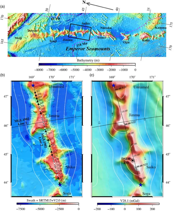
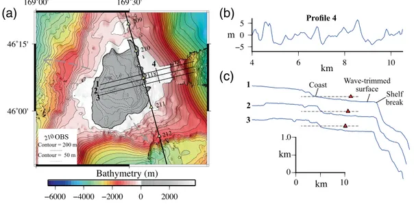
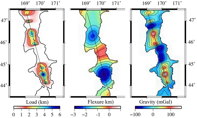
Figure 1. Location maps showing the Emperor seamount chain and MGL1902 Lines 1 and 2 along which OBS, MultiChannel Seismic (MCS) reflection and free-air gravity anomaly data have been acquired. Blue filled stars locate the start/end co-ordinates of the profiles in Figures 3–8, 11 (a) Emperor seamount chain. Bathymetry based on a 100 × 100 m SRTM15 + V2.0 grid (Tozer et al., 2019). Dashed magenta lines show the boundary of Cretaceous Normal Superchron (CNS) oceanic crust. (b) OBS 201–228 and OBS 118 locations and MGL1902 Line 2 ship track (black solid line). White filled triangles are WHOI instruments. Black filled triangles are GEOMAR LOBSTER instruments. Gray filled triangles are GEOMAR ultradeep LOBSTER instruments. Map shows bathymetry based on a 100 × 100 m merged swath and SRTM15 + V2.0 bathymetry grid (Tozer et al., 2019). White lines (contour interval: 1 km) show the flexure based on a simple model of surface volcano loading with a load and infill density of 2,882 kg m⁻³ and an effective elastic thickness of the lithosphere, Te, of 14 km. (c) Free-air gravity anomaly based on a 1 × 1 min satellite-derived V28.1 grid (Sandwell et al., 2019). Black solid line shows MGL1902 Lines 1 and 2.

Tick marks are shown every 6 h along the track. Month/day annotations every 24 h. Flexure is negative down and is annotated every 2 km. OBS, ocean bottom seismometer.

Cretaceous Normal Superchron (CNS) oceanic crust, ∼83–118 Ma in age, suggesting they were emplaced on much younger oceanic crust and lithosphere than the Hawaiian Ridge where the underlying oceanic crust is of similar in age (∼83–93 Ma). Such a tectonic setting is in accord with paleogeographic reconstructions (Wright et al., 2016), which place the Emperor seamounts close to a transform fault that offset the Izanagi/

Pacific and Kula/Pacific spreading ridges, and flexure studies (Watts, 1978; Watts & Ribe, 1984), which show that the Emperor seamounts are associated with relatively low values of the elastic thickness of the lithosphere, Te, in the range 10–20 km.

Previous deep seismic studies have generally confirmed the crustal structure inferred from gravity and flex- ure modeling of hotspot generated ocean islands and seamounts and have provided constraints on the mechanisms of emplacement of submarine volcanoes in an intraplate setting. At Oʻahu and Molokaʻi on the Hawaiian Ridge, the flexed oceanic crust appears to be underplated by magmatic material that is inter- mediate in P wave velocity (and hence density) between lower crust and upper mantle (Watts et al., 1985).

At Hawaiʻi there is evidence of a décollement surface which defines the contact between the base of the volcanic edifice and the top of flexed oceanic crust (Morgan et al., 2003). The Canary and Cape Verde islands do not appear to be underplated (Pim et al., 2008; Watts et al., 1997), but the Marquesas and the Ninetyeast Ridge do (Caress et al., 1995; Grevemeyer et al., 2001a). The Louisville Seamount chain, the northern end of which is similar in age to the Emperor seamounts, is unusual in revealing a high P wave velocity (>7.2–

7.6 km s⁻¹) intrusive body in the lower flexed crust that underlies the edifice (Contreras-Reyes et al., 2010).

All seamounts and ocean islands appear susceptible to large-scale slope failures that generate slump and slide blocks, debris flows and long run-out turbidity currents (Moore et al., 1989; Oehler et al., 2004; Watts

& Masson, 1995).

We recently had the opportunity during cruise MGL1902 of R/V Marcus G. Langseth to acquire a 400-km- long seismic refraction and gravity, swath bathymetry and magnetic anomaly profile along the crest of the Emperor Seamounts, thereby ‘sampling’ the structure of some ∼18% of the length of this hotspot generated seamount chain. We use these newly acquired data to examine the volume and distribution of magmatism that has been added to the oceanic crust along a segment of the Emperor seamounts, the response of the Pacific oceanic plate to volcano loading and its implications for underplating, guyot subsidence and litho- spheric strength.

2. Seismic and Gravity Data

2.1. Ocean Bottom Seismometer Data

Seismic refraction data were acquired using the full 36-element 104.5–108.1 L volume array of Langseth and 29 Ocean Bottom Seismometers (OBSs) deployed along a strike line connecting Suiko and Jimmu guyots (Figure 1b). The array was towed at a depth of 12 m, the shot interval was 400 m and the speed along the strike line was ∼4 knots, except near the northern end of the profile where it was increased to 4.5 knots in order to avoid bad weather. Shots were recorded on short-period seismometers from GEOMAR and Woods Hole Oceanographic Institution (WHOI). Three types of OBS were employed with different water depth ratings: (1) WHOI short periods (5,500 m); (2) GEOMAR LOBSTERS (6,000 m); and (3) GEOMAR ultradeep LOBSTERS (8,000 m). All instruments were deployed by ‘free fall’ using the shipboard Global Positioning System (GPS) for drop point positioning. Instrument locations were further constrained using water path arrival times from airgun shots acquired while the ship was navigated with GPS, and the resulting OBS drift was determined to have been in the range 50–400 m. OBS data were recorded continuously at a sample rate of 5 ms and each OBS successfully recorded the shots.

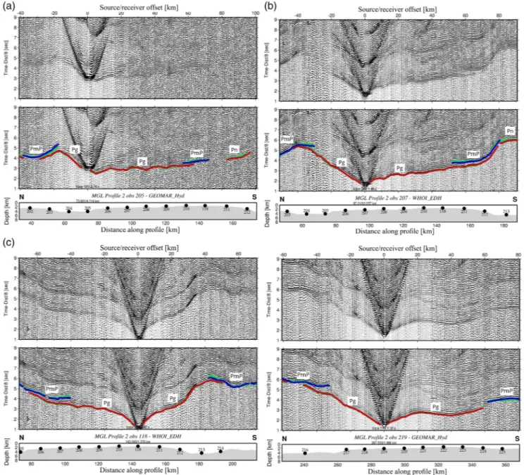
Examples of the original GEOMAR and WHOI OBS wide-angle data are shown in Figure 2. Record sec- tions are affected by strong depth variations of the undulating bathymetry along the crest of the Emperor seamounts, which rises from ∼5.0 km on the south flank of Suiko to ∼1.2 km on its summit. The sections typically show offsets of 80–100 km and recordings are dominated by first breaks with apparent velocities of 6–7 km s⁻¹ at offsets of 15–60 km, suggesting that the seamounts are cored by intrusive rocks, which are overlain by material with apparent velocities of <4–5  km/s, probably reflecting extruded basalts, volcanoclastic and mass wasting deposits. We interpret all branches with velocities of <7 km/s as crustal

arrivals or Pg. At offsets of 20–80 km we observe a prominent secondary arrival, which is interpreted to represent a wide-angle Moho reflection or PmP. At some stations (e.g., Figure 2a, northern branch) PmP oc- curs at 20–40 km, while at others it emerges at >40–60 km (e.g., Figures 2b and 2d). The different offsets of PmP energy clearly supports strong thickness variations of crust along the chain. While the observed appar- ent velocity and character of record sections resembles oceanic crust (Grevemeyer et al., 2018; Christeson et al., 2019) the offsets observed for the PmP along the seamount chain clearly supports a crustal thickness exceeding that of normal oceanic crust.

Figure 2. Examples of original GEOMAR and WHOI OBS wide-angle seismic reflection and refraction data record sections with observed and predicted travel times based on the velocity model in Figure 4. Green solid lines show all observed picks. Red solid lines show calculated first arrival Pg and Pn refractions. Blue solid lines show calculated PmP reflector. Filled black circles locate the OBSs on the seafloor. (a) GEOMAR LOBSTER OBS 205 on the north flank of Jimmu. (b) WHOI OBS 207 on the north flank of Jimmu. (c) WHOI OBS 118 at the intersection of Lines 1 and 2 on the summit of Jimmu. (d) GEOMAR LOBSTER 219 on the north flank of Suiko. Eight additional OBS data record sections are presented in Supporting Information (Figures S1–S8). Pg, crustal arrivals; PmP, Moho reflection; Pn, uppermost mantle; WHOI OBS, Woods Hole Oceanographic Institution ocean bottom seismometer.

2.2. Multichannel Seismic Data

MultiChannel Seismic (MCS) reflection data using the full element array and the 1,188 channel, 14.875-km- long, streamer of Langseth were acquired along a line parallel to and offset by ∼400 m from the OBS line.

The streamer was towed at a depth of 12 m, the shot interval was 62.5 m, the record length 26 s, and the speed along the strike line was ∼4.2 knots. Examples of the original data acquired are shown in Support- ing Information (Figures S9–S13). Two-Way Travel Time (TWTT) record sections reveal an absent or thin (0–0.1 s TWTT, ∼0–0.3 km thickness) pelagic drape on the crest and flank of the guyots. Thicker accumu- lations (up to 0.8 s TWTT, ∼1.2 km thickness) with similar acoustic characteristics are observed in the ba- thymetric depressions that separate Jimmu and Suiko guyots and Jimmu guyot and an unnamed seamount to the north. There is evidence of further sedimentary accumulations along the strike line, for example in the bathymetric depressions, which are characterized by discontinuous reflectors and chaotic bodies. We interpret the discontinuous reflectors as volcanoclastic sediments (with the higher amplitude reflectors representing intercalated flows), and the chaotic bodies as the products of mass wasting on the guyot flanks.

In general, the internal reflectivity of the guyots is weak, although reflectors that represent the top of the extrusives have been identified on both Suiko and Jimmu guyots. The deepest reflectors (7.0–8.5 s TWTT,

∼8.5–11.0 km depth) are found beneath the bathymetric depressions and most likely represent that top of preexisting oceanic crust.

2.3. Free-Air Gravity Anomaly Data

Gravity data along the OBS and MCS strike lines were acquired with a recently refurbished Bell Aerospace BGM-3 gravimeter. The raw pulse rate count were corrected for bias and converted to mGal using values of 852513.49 mGal and 5.096606269 mGal/count respectively. Prior to correcting for latitude and the Eöt- vös effect the data were filtered with a 120 s Gaussian filter in order to eliminate accelerations due to ship motion.

Examples of the BGM-3 gravity data acquired on the summit of Jimmu guyot are shown in Figure 3. The figure shows that the Gaussian filtered data still contains a significant level of ‘noise’, which we removed with a 1.0 km median filter following correction for latitude and Eötvös. The median filtered shipboard BGM-3 data show a strong correlation with the swath bathymetry and better resolves the small-scale fea- tures of Earth’s gravity field than currently available global satellite-derived fields such as DTU10 (Anders- en et al., 2010) and V28.1 (Sandwell et al., 2019). Watts et al. (2020) obtained a similar result in their study of shipboard BGM-3 and satellite-derived gravity data over Jimmu, and other seamounts in the northwest Pacific. We therefore use shipboard rather than satellite-derived gravity anomaly data in this paper.

Figure 3a shows that free-air gravity anomalies over the summit of Jimmu guyot are ∼215 mGal and gen- erally in the range 210–220 mGal, despite a general increase in depth of ∼700 m from south to north along the profile. Similar high amplitude anomalies occur over Suiko where they exceed 300 mGal. The flanks of both guyots are associated with small-scale gravity anomalies (wavelengths <∼25 km), which correlate closely with bathymetry. For example, free-air gravity anomaly ‘highs’ A and B (Figure 3a) over the north flank of Jimmu show amplitudes of ∼5 mGal and correlate with changes in bathymetry of ∼650 m (Fig- ure 3c). Swath bathymetry data (Figure 3b) suggest that these features, which are not resolved in the global satellite-derived fields, are volcanic cones with summit craters that appear to have undergone little mass wasting.

3. Seismic and Gravity Modeling

3.1. Seismic Tomographic Inversion

Travel time data were hand-picked for a joint refraction and reflection tomography analysis. A low ambi- ent noise level and the good quality of waveforms made selection of first breaks relatively straightforward (Figure 4). Upper crustal arrivals could be picked to ∼10 ms, or better, using a similar method to Zelt and Forsyth (1994). However, for larger offsets the signal-to-noise ratio of crustal arrivals (Pg) decreases; middle to lower crustal first breaks generally have picking uncertainties of 40–60 ms. The largest uncertainties of ± 90 ms were assigned to energy turning in the uppermost mantle (Pn) and secondary wide-angle reflections

from the crust-to-mantle boundary or seismic Moho (PmP). For the inversion procedure, we used a lay- er-stripping approach and thus inverted first for the shallow structure using near offsets before the addition of larger offsets and wide-angle reflections. For this top-down approach, picked travel times were assigned to upper, middle and lower crust based on apparent velocity and offset. The Pn arrivals are generally well defined, emerging from the wide-angle Moho reflection (e.g. Figures 2a and 2b).

We invert for the two-dimensional P wave velocity (Vp) structure and the geometry of the seismic reflec- tion Moho along MGL1902 Line 2 using the joint refraction and reflection travel-time tomography code TOMO2D (Korenaga et al., 2000). Initially, two different 1-D starting models were used for the seismic structure below the seafloor. The first was based on normal oceanic crust found in the Pacific Basin (Greve- meyer et al., 2018), while the second approximated the structure of volcanic edifices of seamounts (Contre- ras-Reyes et al., 2010; Weigel & Grevemeyer, 1999). The main differences are that the second model has a much thicker upper crust, which is ∼1.5–2 km thick for oceanic crust and up to 5 km thick for seamounts.

The second model performed much better than the first model and so a Monte Carlo approach was adopted for all inversions. To reduce the number of free parameters, we used regularization and defined a vertical and horizontal correlation length. Vertical correlation length increased from 0.2 km at the top to 1 km at the bottom of the velocity grid; horizontal correlation length increased from top to bottom from 5 km to 10 km.

The base of the model was assumed at 30 km depth.

As indicated above, we chose a layer-stripping strategy (Contreras-Reyes et al., 2010). In the first step, we inverted for the shallow structure of the edifice, which might be highly heterogeneous, reflecting the dep- osition of either low velocity volcanoclastic deposits with intercalated flows or high velocity basaltic ex- trusive and intrusive rocks (Contreras-Reyes et al., 2010; Weigel & Grevemeyer, 1999). After 15 iterations, Figure 3. Examples of the BGM-3 gravity data acquired during the MGL1902 cruise over the crest of Jimmu guyot.

(a) Gravity data. Gray filled circles show pulse rate count 1 s data, corrected for bias and converted to mGal, Gaussian filtered with a 120 s filter prior to correcting for Eötvös and Latitude. Red solid line show a postcorrection median 1 km filter. Dashed color lines show the DTU10 (Andersen et al., 2010) and V28.1 (Sandwell et al., 2019) 1 × 1 min satellite-derived gravity anomaly fields. (b) Swath bathymetry based on a merge of data acquired on MGL1902 Line 2 and the global combined SRTM15 + V2.0 shipboard and satellite-derived bathymetry derived by (Tozer et al., 2019). (c) Comparison of the swath bathymetry 10 s center beam data (solid blue line) to the global SRTM15 + V2.0 bathymetry (dashed blue line).

(a)

(b)

(c)

we obtained a travel time Root Mean Square (RMS) misfit of ∼0.07 s and a chi-square (χ²) of <3, revealing a large degree of heterogeneity in the shallow structure and perhaps some three-dimensional travel time effects that have been condensed into a two-dimensional model. For the inversion of all crustal Pg arrivals we used 10 more iterations and obtained a RMS of ∼0.080 s and a χ² of <2 (Table 1). However, oceanic crust Figure 4. Results from the Monte Carlo inversion along MGL1902 Line 2 of the Emperor Seamount chain (Figure 1).

(a) Average model obtained from 100 inversion runs. P wave velocity contoured at 0.5 km s⁻¹ interval. Green line marks the upper limit of Moho and red line the lower limit. Average Moho is indicated by black solid line; (b) Cell hit counts of the Moho as obtained from the 100 models runs. Red areas are well-resolved segments, indicating that models stack at a similar depth. (c) RMS in velocity uncertainty from the 100 model realizations. (d) Derivative Weight Sum (DWS) of the average crustal tomographic model, which provides a proxy for the distribution of the refracted and reflected energy traced through the model.

(a)

(b)

(c)

(d)

and seamounts generally show a low gradient lower crust (Grevemeyer et al., 2018) and therefore provide little resolution at the base of the crust.

Therefore, the velocity structure at the base of crust is largely constrained by jointly inverting crustal arrivals (Pg) and Moho reflections (PmP). Af- ter eight more iterations, the inversion yielded a RMS of ∼0.085 s (Fig- ure A1) and a χ² of ∼1.1 (Table 1).

Uncertainty of the crustal velocity model and Moho depth (Figure 4) were assessed by means of a Monte Carlo analysis (Korenaga et al., 2000).

We followed the same layer-stripping strategy used to obtain an average model and estimate the uncertainty of each grid cell. We tested a random 100 cases, each of which was derived from a one-dimensional crustal Vp- depth profile and a flat reflector as the initial model. We applied a random perturbation of ±10% and ±6% for upper and lower crustal velocities, respectively. Most domains of the model show a reasonably small RMS uncertainty of <0.1 km s⁻¹ (Figure 4c), with maximum values of 0.2 to

<0.3 km s⁻¹ (Figure 4c) reached where the high gradient upper crustal velocity grades into a more moderate gradient at mid-crustal level. Furthermore, in some areas of poor coverage larger uncertainties are observed at the base of crust, reaching values of 0.1–0.2 km s⁻¹. The seismic Moho shows clear variations and its uncertainty varies from just ±0.5 km at 50 km to 85 km and 170 km to 260 km (Figure 4), reaching its max- imum uncertainty of ±2 km beneath Suiko guyot and 1.5 km beneath Jimmu guyot.

The resulting tomographic model shows some unusual features. Most prominent are very large heteroge- neities in the uppermost 2–4 km of the model, where velocity varies from ∼3 km s⁻¹ in some small basins to >6.5 km s⁻¹ in the main guyot edifices. We believe these heterogeneities to be real, and it is reasonable to suggest that the low velocity anomalies represent volcanoclastic or mass wasting deposits while high ve- locity anomalies mark intrusions. Another unusual result is the homogeneity of the velocity model 5–6 km above the Moho, showing velocities of >6.5–7.2 km s⁻¹, which may reflect, in part, the preexisting oceanic crust. However, the velocity model does not show any clear discontinuity between the heterogeneous upper crust and the more homogeneous lower crust, but reveals a rather gradual transition at mid-crustal levels.

Beneath the tall guyot edifices, roughly at >4 km below seafloor, the 6 km s⁻¹ and 6.5 km s⁻¹ iso-velocity contours may mark the transition from a high gradient upper crust to a lower gradient lower crust and hence may characterize the transition from relatively low porosity extrusive and clastic basaltic deposits above to relatively low porosity basalt or gabbros. Therefore, high velocity and, hence, dense material is forming an integral part of the edifices.

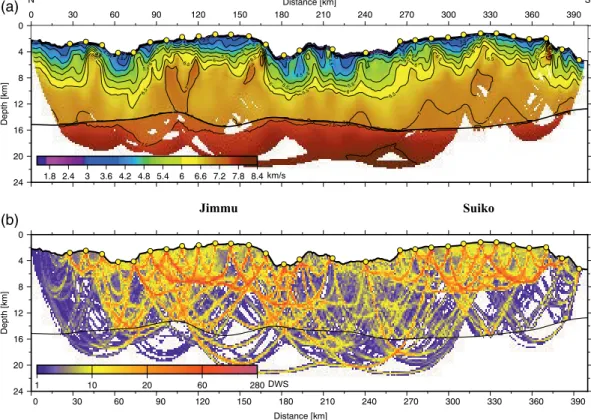
The upper mantle velocity structure (Figure 5), beneath the main guyot edifices, was derived using a grid search of mantle velocity ranging from 7.4 to 8.2 km s⁻¹ and damping the average crustal model and hence keeping the crustal structure essentially unchanged while inverting for mantle structure. In general, the mantle is reasonably homogeneous with a mantle velocity below Moho of 7.9–8.0 km s⁻¹ increasing with depth. However, below the northern flank of Jimmu, there is a region of mantle with relatively low velocity of 7.5–7.6 km s⁻¹. This localized region of low velocity is a robust feature of all model runs during the grid search. Uncertainty of mantle velocity is < 0.1 km s⁻¹, of the order of 0.05 km s⁻¹.

3.2. Gravity Modeling

The seismically constrained crust and mantle structure has been verified by forward gravity modeling. We used the P wave velocity structure in Figure 4 to subdivide the crustal structure into seven subseafloor in- terfaces. The average P wave velocity of each interface-bounded layer was then calculated and the average density of the layer estimated using the empirical equations of Nafe and Drake (1963) and Christensen and Mooney (1995) for P wave velocity in the range 1.6–6.0 km s⁻¹ and 6.0–8.2 km s⁻¹ respectively, as summa- rized in Brocher (2005). We selected Christensen and Mooney (1995) because it is based on a large number of observations of seismic refraction/wide-angle reflection profiles from crystalline rocks including basalt, diabase, gabbro and dunite, which are the rock types that we would expect at seamounts, and because its density and velocity relationship have been used with some success to verify theoretical predictions based on mineral physics (Hacker et al., 2003). The final steps were to calculate the density contrast across each Phase No. of Observations RMS^a (s) Chi-square^a χ²

Pg¹ 2,548 0.061–0.072 1.76–2.40

Pg 5,187 0.067–0.110 1.33–3.18

Pg + PmP 7,633 0.080–0.088 1.10–1.35

Pg, PmP + Pn 8,872 0.086–0.100 1.17–1.52 Pg¹, Arrivals that turn in the upper crust; Pg, crustal arrivals; PmP, Moho reflection; Pn, uppermost mantle.

aMinimum and maximum values of the 100 random models after inversion.

Table 1

Summary Table With Misties Between Arrival Picks at all OBSs Along MGL1902 Line 2 and Model Predictions

interface, to use a line-integral method based on a semi-infinite horizontal sheet of mass with a sloping edge (Talwani et al., 1959) to calculate the gravity effect of each interface, and sum the effects for all the interfac- es, and compare the sum to the observed free-air gravity anomaly (Figure 6).

Figure 6 shows a close agreement between the observed free-air gravity anomalies and the calculated gravity anomalies based on the seismically constrained crustal structure. We point out that no attempt was made in the calculations to modify, in any way, the seismically constrained structure so as to improve the fit between observed and calculated gravity anomalies. The figure shows that the calculated anomaly explains well both the amplitude and wavelength of the observed anomaly over the summits of Jimmu and Suiko guyots. The RMS difference between observed and calculated gravity anomalies is 19.5 mGal, and the main discrepan- cies appear confined to 80–120 km over the north flank of Jimmu, 180–260 km in the deep-water region between the Suiko and Jimmu and 330–400 km over the south flank of Suiko.

A potential problem with the calculation in Figure 6 is the assumption of two-rather than three-dimension- ality. Dimensionality becomes significant if the strike length of a causative body is small in comparison to its width. The strike length and width of Jimmu and Suiko along MGL1902 Line 2 are approximately equal (∼60–80 km) and so dimensionality may be a factor in the gravity calculations. Bathymetry data were ac- quired over a swath of the seafloor but the seismic data are limited to a single line. The only interface with a known extent in three-dimensions is therefore the seafloor.

Figure 7 shows the gravity effect of the individual layers that were used to calculate the free-air gravi- ty anomaly in Figure 6. The gravity effect of the seafloor was computed assuming the two-dimensional line-integral method of Talwani et al. (1959) (dashed blue line, Figure 7b) and the three-dimensional Fast Fourier Transform (FFT) method of Parker (1972) (solid blue line, Figure 7b). The RMS difference be- tween the gravity effects is 9.1 mGal, with the largest discrepancies over the deep-water between Jimmu and an unnamed seamount to the north and between the summits of Jimmu and Suiko, regions where swath Figure 5. Two-dimensional seismic Vp tomographic model along-strike of the Emperor seamount chain, crossing Jimmu and Suiko guyots. Solid black line shows the average Moho. (a) Average model obtained from 100 inversion runs. P wave velocity contoured at 0.5 km s⁻¹ interval. (b) DWS and hence ray coverage of the average crustal and mantle tomographic model. DWS, Derivative weight sum; Vp, P wave velocity.

(a)

(b)

bathymetry data suggest significant changes in bathymetric contours either side of the seismic line. While three-dimensional effects could therefore contribute up to half of the RMS difference between observed and calculated gravity in Figure 6a, we believe the close agreement between them is representative and confirms the validity of the seismically derived crustal structure, as presented in Figure 4.

In addition to the gravity effect of the seafloor, Figure 7b also shows the contributions to the calculated anomaly of the gravity effect of the seven individual, seismically constrained, subseafloor interfaces. The figure shows that interface 5, which is defined by the 6 km s⁻¹ iso-velocity contour, is the largest contributor to the calculated gravity effect of the subseafloor seismic structure with an amplitude over Jimmu and Suiko almost as large as that of the seafloor. Other significant contributions are from the 7 km s⁻¹ iso-velocity Figure 6. Comparison of the observed and calculated gravity anomaly based on the crustal P wave velocity model in Figure 4a. (a) Observed BGM-3 free-air gravity anomaly (gray filled circles shows the 120 s Gaussian filtered 1 s data. The red line shows a 1.0 km median filter. Black solid line shows the calculated gravity anomaly based on the density layers in b). (b) P wave velocities at 1 km s⁻¹ interval derived from the crustal model in Figure  4c. (c) Crustal model from tomographic inversion. Solid purple line shows the best fit average Moho and the dashed purple lines show minimum and maximum bounds.

(a)

(b)

(c)

(a)

(b)

(c)

contour (interface 6, Figure 7b) and the combined contributions of the 2–5 km s⁻¹ iso-velocity contour (interfaces 1–4, Figure 7b).

We noted earlier for the crust-only model in Figure 6 that the main discrepancies between observed and calculated gravity anomalies occur over the deep-water region between Jimmu and Suiko, the north flank of Jimmu and the south flank of Suiko. We therefore computed the gravity effect of the combined crust and mantle seismically constrained model (Figure 5) and compared it to the observed free-air gravity anoma- lies. Figure 8a shows an improvement in the fit between observed and calculated gravity, especially over the deep water region between Jimmu and Suiko and the north flank of Jimmu. The RMS is reduced from 19.5 mGal for the crust model to 17.2 mGal for the crust and mantle model and the gravity effect of the small modifications in the configuration of the 7 km s⁻¹ velocity contour leads to a better fit to the gradients over the flanks of the guyots. Interestingly, the inclusion of a low density body in the uppermost mantle beneath the north flank of Jimmu, as suggested by the 7.5 km s⁻¹ iso-velocity contour, reduces the gravity anomaly high associated with the 7 km s⁻¹ intrusive body and improves the overall fit.

4. Discussion

4.1. Intrusives Versus Extrusives

Seismic and gravity models have the potential to reveal information on the composition of seamounts and the amount of magmatic material added to the preexisting Pacific oceanic crust. Previous studies (Ham- mer et al., 1994; Weigel & Grevemeyer, 1999) show that the subseafloor average P wave velocity structure of seamounts is significantly lower than normal oceanic crust at the same depth. The low velocities have been interpreted in terms of low densities and high porosities due to the shallower water eruptions that occur at seamounts than occur at a mid-ocean ridge, and the extrusion of lavas, hyaloclastites and clastic material derived by mass wasting and submarine landsliding. At greater depths (2–3 km on Great Meteor and 4–5 km on Jasper) higher P wave velocities (>6.0 km s⁻¹) are encountered and have been interpreted by Weigel and Grevemeyer (1999) and Hammer et al. (1994) as intrusives of gabbro or ultramafic rocks.

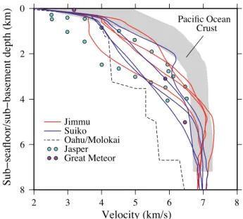
Figure 9 compares four P wave velocity versus depth profiles from the summits of Suiko and Jimmu guyots to profiles of other seamounts and oceanic islands and to normal Pacific Ocean crust. The Suiko and Jimmu profiles were derived from the crust and mantle model in Figure 8. The seamount profiles in the figure are from Jasper in the eastern Pacific (Hammer et al., 1994) and Great Meteor in the central Atlantic (Weigel

& Grevemeyer, 1999), and the normal Pacific Ocean crust is based on a recent compilation of wide-angle seismic refraction data by Grevemeyer et al. (2018). The figure shows that the Suiko and Jimmu profiles overlap those of Jasper and Great Meteor, and the summits of both guyots are consistently lower in velocity than normal Pacific oceanic crust. High P wave velocities (>6.5 km s⁻¹) are encountered at depths ∼3–6 km beyond which the Suiko and Jimmu profiles overlap normal Pacific Ocean crust.

We follow Hammer et al. (1994) and Weigel and Grevemeyer (1999) and interpret the low P wave velocities (2–4 km s⁻¹) at Suiko and Jimmu in terms of low densities and high porosities associated with extrusive lavas and clastic material formed during shallow water eruptions: conditions that would have prevailed during guyot formation. Comparisons with the Staudigel and Schmincke (1984) model for seamount evo- lution suggest that the intermediate velocities (4–6 km s⁻¹), which are still low in comparison with Pacific Ocean crust at the same depth, comprise extrusive lavas with small-scale intrusions. The high velocities (>6.0 km s⁻¹), which overlap normal Pacific Ocean crust, correspond to the deep-water shield building phase and represent, we believe, intrusive gabbros and possibly ultramafic rocks with sheeted dikes.

4.2. Oceanic Crust Thickness, Flexure and Elastic Thickness, Te

Seismic and gravity models of crustal structure at seamounts have potential to constrain the long-term strength of the lithosphere. By comparing observed seismic and gravity data to predictions based on elastic Figure 7. Gravity effect of the individual interfaces between the seismically constrained crustal layers. (a) Observed (red) and calculated (black) free-air gravity anomalies. (b) Gravity effect of the individual crustal interfaces which include the seafloor and seven subseafloor interfaces. Solid and dashed blue lines show the two-dimensional and three-dimensional gravity effect of the seafloor respectively. Numbers show the average P wave velocities above and below the interface and the density contrast assumed across the interface. (c) P wave iso-velocity contours, layers and densities assumed in the gravity calculations.

Figure 8. Comparison of the observed and calculated gravity anomaly based on the combined crust and mantle P wave velocity model in Figure 5a. (a) Observed BGM-3 free-air gravity anomaly (gray filled circles shows the 120 s Gaussian filtered 1 s data and the red line shows the 1.0 km median filter. Black solid line shows the calculated gravity anomaly based on the density layers in b). Black dashed line shows the calculated gravity anomaly of the crust-only P wave velocity model in Figure  4b. (b) Calculated gravity effect of the individual layers that comprise the crust and mantle structure. (c) P wave velocities at 1 km s⁻¹ interval derived from Figure 5 together with the densities assumed for the individual layers. (d) P wave velocity model from Figure 5.

(a)

(b)

(c)

(d)

and viscoelastic plate flexure models it is possible to estimate the effec- tive elastic thickness of the lithosphere, Te: a proxy for its long-term ther- mal and mechanical strength. Previous Te estimates from the Emperor Seamounts have been based only on gravity and geoid data. Watts (1978) used shipboard gravity measurements, projected bathymetry profiles and two-dimensional continuous plate models to show that the Emperor Sea- mounts in the vicinity of Tenji, Jimmu, Suiko, Nintoku, Ojin and Koko are associated with relatively low values of Te, in the range 10–20 km.

Watts and Ribe (1984) carried out a three-dimensional study using a SEA- SAT satellite-derived geoid of Ojin and Suiko and obtained a best fit Te of 17 and 10 km respectively. Calmant (1987) carried out a similar study of Ojin and Suiko and obtained a best fit Te of 19 and 18 km respectively.

These relatively low values of Te compared to those obtained at the Ha- waiian Ridge (20 < Te < 32 km) were interpreted by Watts (1978) as indi- cating that the Emperor Seamounts formed on young oceanic lithosphere at, or in close proximity to, a spreading ridge.

It is usual in seamount flexure studies to define the ‘driving load’ as the present day bathymetry above some ‘base’ (usually the mean depth) and the ‘infill’ load as the material that infills the flexural depression. In the case of an across-strike (i.e. dip) profile of a seamount, the infill load needs to be specified beneath both the ‘driving’ load and the flanking moats. However, for an along-strike profile, such as MGL1902 Line 2, it is the ‘infill’ load immediately beneath the ‘driving’ load that is most im- portant and will exert the largest control on the flexure. If the density of the ‘driving’ load and the infill load are known, for example from seismic and gravity modeling, then the flexure along a strike line can be comput- ed from the present day bathymetry for different values of Te. The depth to the top of the flexed oceanic crust is given by Wd + w where w is the flexure and Wd is the mean depth of the bathymetry and the predicted Moho depth is given by Wd + w + Tc, where Tc is the thickness of the preexisting flexed oceanic crust which is assumed constant along the length the profile. Because our P wave velocity models do not show a clear discontinuity marking the top of the preexisting crust, Tc, like Te, is an elastic thickness that needs to be solved for.

Figure 10 shows a plot of the RMS difference between observed seismic Moho and the calculated flexed Moho along MGL1902 Line 2 assuming the present-day bathymetry, a driving load of equal density to the infill load, and different values of the elastic thickness: Tc and Te. The calculations are based on a merged swath grid, a ‘driving’ and ‘infill’ load density of 2,882 kg m^-3 (as derived, for example, in the seismic and gravity modeling of the main part of the Suiko and Jimmu edifice in Figure 6) and a mean depth of the pres- ent-day bathymetry, Wd, of 5,260 m. The parameter pair (marked by a red filled star in the figure) that gives the lowest RMS (760.8 m) is for Tc = 5.1 km and Te = 14 km. The Tc is consistent with the estimate of ∼5 km by Dunn et al. (2019) along MGL1902 Line 1 (which intersects MGL1902 Line 2 at OBS 118, Figures 1b and 1c) and the Te is within the range of the estimates of Watts (1978) and Watts and Ribe (1984) of (10–20 km) based on gravity and geoid data.

We have used the results from flexure modeling to interpret the seismically constrained crust and mantle models in terms of the deep structure of Jimmu and Suiko guyots in Figures 11c. The blue shaded region in the figure, which shows the depth, thickness and shape of the preexisting oceanic crust as derived from the best fit flexure model, highlights the total amount of magmatic material that has been added to the top, base and within the flexed oceanic crust. The red shaded region shows the material we interpret as mainly intrusives and the yellow/brown region the overlying material mainly extrusives and clastics. Together, the intrusives and extrusives represent mainly magmatic material added to the top of the preexisting oceanic crust. In contrast, there appears to have been little material added to the base of oceanic crust, except be- neath the north flank of Jimmu where there is a region of relatively low mantle velocities. We interpret the low velocities as melts, which may be related to a younger phase of volcanism, as suggested in the swath Figure 9. Comparison of selected subseafloor velocity versus depth

profiles for Suiko (Solid blue lines) and Jimmu (Solid red lines) guyots to other seamounts and normal Pacific Oceanic crust. The profiles were constructed at distances of 100, 120, 140, and 160 km (Jimmu) and 300, 320, 340, and 360 km (Suiko) along MGL1902 Line 2 (Figure 8). The seamount data are from Jasper (Hammer et al., 1994), Great Meteor (Weigel and Grevemeyer, 1999) and O’ahu/Moloka’i (ten Brink and Brocher, 1987). The Pacific Ocean crust data (gray shade) is based on the compilation of Grevemeyer et al. (2018).

bathymetry data (Figures 3b and 3c) which reveal a number of circular volcanic cones with summit craters on the seafloor above the region of low velocity. We do not see any evidence for magmatic underplating of the preexisting oceanic crust, at least not on the scale described by Watts et al. (1985), Ten Brink and Brocher (1987) and Leahy et al. (2010), for example, in the region of Oah’u and Moloka’i on the Hawaiian Ridge and by Caress et al. (1995) at Marquesas and Grevemeyer et al. (2001a) at the Ninetyeast Ridge.

There is, however, evidence of intrusive bodies within the main edifice (Figures 11c) similar in dimensions to those modeled from gravity data and described by Kellogg et al. (1987) from two large guyots in the west- ern Pacific and Flinders et al. (2013) from the Hawaiian Islands. Intru- sive bodies are also found within the underlying preexisting flexed crust.

But, as we pointed out previously, the lowermost 5–6 km of the crust beneath Jimmu and Suiko is remarkably homogeneous in its P wave ve- locity structure with velocities in the range 6.5–7.2 km s⁻¹. We do not therefore see evidence of velocities exceeding ∼7.2 km s⁻¹, as has been described by Contreras-Reyes et al. (2010), for example, from beneath the Louisville Ridge.

The absence of magmatic underplating and lack of a high velocity and, hence, high density preexisting crust beneath Suiko and Jimmu guyots is of interest because it is generally considered that a significant pro- portion of hotspot magmatism is formed from melt trapped or intruded near the base of the crust. Basalts generated, for example, from abnor- mally hot mantle and rich in magnesium typically exhibit high velocities and, hence, densities when they crystallize (Keleman & Holbrook, 1995;

White & McKenzie, 1989). The preexisting crust-mantle boundary forms a significant density contrast, so it is likely that melts generated at depth in a plume will eventually accumulate near its base where they either underplate the flexed crust or intrude it. High velocity lower crust is ob- served at a large number of seamounts, but may not form an integral part of all seamounts and ocean islands as several, like the Emperor Seamounts, do not reveal either a magmatic underplate or a high velocity crust (Grevemeyer et al., 2001b; Operto & Charvis, 1996; Watts et al., 1997).

The mechanisms controlling the formation of high P wave velocity oceanic crust at seamounts and oceanic islands remains therefore enigmatic.

A problem with the flexure model, highlighted in Figures 11c is that despite the well-defined RMS mini- mum between the observed seismic and calculated flexed Moho, the fit between the observed free-air gravity anomaly (red solid line) and calculated gravity effect of the flexure model (green dashed line in Figures 11a) is poor, especially over the guyot summits where the calculated gravity underestimates the observed gravity by up to ∼100 mGal. This is the case despite our use in the flexure modeling of a high density for the edifice (2,882 kg m^-3) based on the seismic P wave velocities. This suggests the difference in gravity anomalies is not due to an uncertainty in the load (and hence infill) density, but to the size of the load itself. The present day bathymetry, which is a product of all the processes that have modified the guyot since it formed may not, therefore, be the best estimator of the load that displaced water and flexed the crust and lithosphere at the time of volcano loading. A better representation of the load might be subseafloor, notably the 6 km s⁻¹ ve- locity contour, as indeed suggested by gravity modeling (Figure 7b) which shows this interface contributes at least as much to the observed gravity as the bathymetry and the fact that we have interpreted it as defining the upper surface of the mainly intrusive material.

In order to test this, we used the 6 km s⁻¹ velocity contour to construct the load assuming it was this load, not the present day bathymetry, that displaced water, flexed the lithosphere and produced the free-air grav- ity anomaly observed today (see Appendix A for load construction details). Figures 11a (blue dashed line) shows that such a load is sufficiently large to explain the observed gravity anomaly over both the crest and Figure 10. Plot of RMS difference between the observed seismic Moho

(Figures 6–8, average Moho) and the calculated Moho based on a simple model of flexure as a function of Tc and Te. The calculations are based on a merged 25 × 25 m grid of MGL1902 swath bathymetry and SRTM15 + V2.0 (Tozer et al., 2019) data, a mean depth of water of 5,260 m and a driving load based on the present day bathymetry and a load and infill density of 2,882 kg m⁻³. The RMS minimum (760.8 m) is indicated by a red filled star and corresponds to values of Tc and Te of 5.1 and 14.0 km respectively. Tc, thickness of the preexisting flexed oceanic crust; Te, elastic thickness.

flanks of Jimmu and Suiko guyots. We caution, however, it is likely that other subseafloor loads, such as those defined by the 4 and 5 km/s refractors (yellow and orange shaded regions in Figures 11c) and which we have interpreted in terms of mainly extrusive lavas and clastics, may also contribute to the gravity anom- aly, but such loads would worsen the fit to the steep gradients of the guyot flanks as they extend much further laterally than the 6 km s⁻¹ load, probably because they represent at least in part the mass wasting products of the main edifice.

A consequence of the larger 6 km s⁻¹ load is that while it explains the amplitude of the gravity anomaly it would increase the flexure and worsen the fit between the observed seismic and calculated flexed Moho.

We tested this by calculating the RMS difference between observed seismic and calculated flexed Moho and between observed and calculated gravity anomaly for the same range of Te and crustal thickness as tested in Figure 10, but using a load defined by the 6 km s⁻¹ refractor rather than the present day bathymetry Fig- ure 12. Results show a well-defined Moho RMS minima. But, the gravity anomaly RMS lacks some minima, because of its lack of sensitivity to Tc. Seismic and gravity minima overlap for 20 < Te < 35 km and 5.4 <

Tc < 5.9 km and so our data are compatible, for example, with an increase in Te to 21.1 km and a Tc of 5.5 km.

However, refraction data will be required along a dip line of Jimmu and Suiko guyots, away from the main flexure, before we will be able to constrain Tc and, hence, Te of the underlying crust and lithosphere.

4.3. Volume of Edifice and Plume Flux

Irrespective of uncertainties in modeling the loads, flexure modeling is useful as it reveals the amount of magmatic material that has been added to the top and bottom of the flexed crust and the amount material Figure 11. Summary crust and mantle structure along MGL1902 Line 2 based on seismic and gravity modeling. (a) Comparison of observed and calculated free-air gravity anomaly. The observed anomaly (solid red line) is based on the filtered BGM-3 data. The calculated anomalies are based on the best fit simple model of flexure with a driving load defined by the present day bathymetry (dashed green line) and the 6 km s⁻¹ iso-velocity contour (dashed blue line).

(b) Merged swath and SRTM15 + V2.0 bathymetry. (c) Crust and mantle structure showing the extent of the mainly sediment drape (yellow shade), the extrusives (green + orange shade), the intrusives (red shade with ‘V’) and the underlying preexisting flexed oceanic crust (blue shade) based on Tc = 5.1 km and Te = 14 km (Figure 10). Also shown are the crustal intrusives beneath Jimmu and Suiko (dark magenta shade) and the low density mantle body beneath Jimmu’s north flank (light magenta shade). Thick black, magenta and blue lines show base of pelagic ooze, an intraextrusive horizon, and top preexisting flexed oceanic crust respectively based on an interpretation of depth-converted picks of prominent reflectors on the MCS profile acquired along MGL1902 Line 2 (Supplementary Material). The brown filled arrows highlight bathymetric features ‘A’ and ‘B’ in Figures 3b and 3c which are interpreted as volcanic cones younger in age than the edifice of Jimmu. The cones maybe related to the low density mantle body and to an intrusive body in the preexisting flexed oceanic crust. Tc, thickness of the preexisting flexed oceanic crust; Te, elastic thickness.

(a)

(b)

(c)

that has intruded into the crust. The areal extent (and volume) of this material is important for assessing magma generation rates and the flux of the plume that generated the Emperor Seamounts.

We can estimate the areal extent (and volume) from the seismic and grav- ity model, for example, in Figures 11c. The area between the 6 km s⁻¹ iso-velocity contour and the top of flexed crust (red shaded region in the figure), which we have interpreted as magmatic material associated with the main shield building event, is 579.7 and 704.3 km² beneath Jimmu and Suiko guyots respectively, and so, if we include the area bounded by the 4 and 5 km s⁻¹ refractors, the total amount added is 2,485.9 km². The seamount width normal to MGL1902 Line 2 is ∼50–60 km (Figure 1), assuming it to be constant, then gives a total volume of 1.24  ×  10⁵– 1.49 × 10⁵ km³. The length of MGL1902 Line 2 is 400 km so if the slope of the along-track distance from Loihi’i plotted against age is 57 km Myr⁻¹ (O’Connor et al., 2013) then the Suiko-Jimmu segment of the Emperor seamounts sampled seismically line took ∼7 My to form. The volume flux is therefore in the range 0.56–0.68 m³ s⁻¹ which is significantly smaller than the ∼4 m³ s⁻¹ estimated by Van Ark and Lin (2004) for the Em- peror seamounts based on a Bouguer admittance method. Rather than using gravity, Wessel (2016) used a bathymetry data set and flexure con- siderations to re-evaluate the volume flux along the Hawaiian Ridge, finding his estimates to also be smaller (by ∼2–3 m³ s⁻¹) than those of Van Ark and Lin (2004). Our estimates for the Emperor seamounts are similar to the estimates of Wessel  (2016) of 0.0–1.0  m³ s⁻¹ for the old end (32–42 Ma) of the Hawaiian Ridge. Wessel (2016) estimated rates of 2.5–10.0  m³  s⁻¹ at the young end (0–6  Ma) of the Hawaiian Ridge, which therefore suggests that the flux through most of the preserved his- tory of the Hawaiian plume has been low. Peaks of up ∼4 m³ s⁻¹ above background in the flux during 0–6 Ma, 12–16 Ma and 25–29 Ma were recognized by Wessel (2016) and attributed by them to plate kinematic changes due, for example, to the Chron 5A reorganization on a spreading ridge in the South Pacific. We find, however, no equivalent peak above the background during the formation of Suiko and Jimmu in the Late Cretaceous–Paleocene, despite an intraoceanic subduction zone system involving trench roll-back develop- ing along a 3,000 km long region that now extends from Hokkaido, Japan across Sakhalin to Kamchatka and into Russia (Domeier et al., 2017).

4.4. Subsidence

Suiko and Jimmu have generally flat tops, as do a number of other Emperor Seamounts, which have been interpreted as wave-trimmed oceanic volcanoes that have subsequently subsided below sea-level (Smoot, 1982). Figure 13 (red dashed line) shows that compared to Koko (∼318 m) at the southern end of the chain, Suiko and Jimmu have subsided an additional 1700 m. Detroit (∼2,300 m), at the northern end of the chain, has subsided an additional ∼1982 m. Recent age models (Muller et al., 2008; O’Connor et al., 2013) suggest that the Emperor Seamounts were emplaced during the Late Cretaceous on or in close proximity to CNS crust. Detroit is ∼76 Ma (O’Connor et al., 2013) and is located on 106 Ma crust while Koko is ∼48 Ma (O’Connor et al., 2013) and is located on 121 Ma crust. Therefore, Detroit formed on ∼30 Ma oceanic crust and lithosphere near the Pacific-Izanagi ridge and so would have been expected, on the basis of the cooling plate model (Parsons & Sclater, 1977), to have subsided an average of 1,364 m since it formed while Koko formed on ∼73 Ma oceanic lithosphere and so would have been expected to subside an average of ∼531 m since it formed (Table 2). The expected difference in subsidence between Koko and Detroit would then be ∼833 m, which is less than half of the observed difference (1982 m) suggesting other contributing factors to the subsidence.

The bathymetry profile in Figure 13 is based on the global SRTM15 + V2.0 grid of Tozer et al. (2019) and so may not be a true reflection of summit depths, especially on Jimmu and Suiko where there has been little Figure 12. Comparison of the RMS difference between observed seismic

Moho and calculated depth to flexed Moho (solid white line contours) with the RMS difference between observed and calculated gravity anomaly (colors) as a function of Tc and Te based on a driving load grid defined by the depth to the 6 km s⁻¹ refractor and a driving and infill load density of 2,882 kg m^-3. Filled red star shows the RMS minimum derived assuming a driving load based on the present day bathymetry (Figure 11). Filled green star shows the selected RMS minimum. Gray dashed line traces out the seismic minima. Tc, thickness of the preexisting flexed oceanic crust; Te, elastic thickness.

previous swath data. We therefore used the swath bathymetry data acquired during the MGL1902 cruise to re-examine the morphology of the summits of Jimmu and Suiko guyots. Figure 14c shows, for example, that Jimmu is characterized by a well-developed wave-trimmed surface at depths of 1,500–1,650 m. The surface, which is shown by the white shaded region in Figure 14a, can be traced all around the guyot where it forms a narrow insular shelf. If we assume that the 1,500 m bathymetry contour corresponds to the former posi- tion of a shoreline (i.e., zero depth) then the shelf break is at a depth of ∼150 m in the east and ∼100 m in the west. The gray shade region in Figure 14a represents bathymetry shallower than 1,500 m and shows the approximate outline of the island at the time when the wave-trimmed surface was formed. The island was elongate in a north-south direction with a maximum elevation of ∼300 m and has prominent embayments in its northwest and southeast coastlines, downslope of which is evidence of submarine landsliding and sediment deposition.

The former shoreline position is located at 1,500 m below present day sea-level, which is nearly twice the expected depth based on the guyot age and thermal cooling models (Figure 13, Table 2). Therefore, other factors must have contributed to the subsidence. Unfortunately, we do not know the path of the subsidence (the 1,500 m contour, for example, depicts only the most recent shoreline) or whether it was initiated dur- ing or following volcano loading. Viscoelastic models of surface submarine volcano loading predict a rapid early subsidence and then a more slowly decreasing subsidence (Watts & Zhong, 2000) which may, depend- ing on initial volcano height, exceed the subsidence predicted by thermal cooling models after a few tens of My. Indeed, the biostratigraphic data at DSDP Site 433 on Suiko (Butt, 1980) suggest an abrupt change from shallow to deep water marking the end of reef growth and a rapid subsidence (compared to normal oceanic crust) during the Eocene through early Miocene. Other possible contributors to the subsidence are that Jimmu formed on the crest of a mid-plate topographic swell, similar in height to the Hawaiian swell, Figure 13. Bathymetry profile along the approximate summits of the Emperor Seamounts based on the global SRTM15 + V2.0 bathymetry grid (Tozer et al., 2019). Profile is located in the inset of Fig.1. Red dashed line shows the general trend of the summit depths which increase from ∼313 m at Koko near the Hawaiian-Emperor bend to

∼2,300 m at Detroit near the western Aleutian trench. Blue dashed line shows the expected depth of Cretaceous Normal Polarity oceanic crust based on a cooling plate model. Magenta dashed line shows the expected seamount summit depth assuming the cooling plate model and taking into account the age of the seamounts and the underlying oceanic crust (Table 2). ‘X’ marks the 1,500 m contour, which is interpreted as defining the coast of the former Jimmu island.

Seamount Age^a (Ma) Age of ocean

crust^b (Ma) Age of crust at time

of loading (Ma) Depth of ocean crust at

time of loading^c (m) Depth of ocean crust at

present day^c (m) Subsidence (m)

Koko 48 121.4 73.4 5,405.6 5,937.0 531.4

Suiko 61 114.9 53.9 5,043.5 5,886.5 843.0

Jimmu 65 114.4 49.4 4,942.8 5,882.4 939.6

Detroit 76 106.4 30.4 4,427.9 5,812.0 1,364.1

a(O’Connor et al., 2013). ^b(Muller et al., 2008). ^c(Parsons & Sclater, 1977).

Table 2

Expected Subsidence of Selected Emperor Seamounts Based on Thermal Cooling Models

and has since migrated off it due to plate motions and that Jimmu, once formed, found itself in the flexural depression of the next major volcano, Suiko, and so underwent an additional subsidence, similar to that now being experienced by Mau’i due to loading of the big island of Hawai’i.

Irrespective, excess subsidence is consistent with our seismic data and the absence of any evidence for magmatic underplating, which would as Grevemeyer and Flueh  (2000) and Ito and Clift  (1998) have demonstrated at oceanic plateaus, thicken the crust and cause uplift. An outstanding question is the role played by the relatively high P wave velocity and hence, relatively dense, intrusions in the middle and lower crust that we have modeled beneath Jimmu and Suiko guyots. Hot melts that intrude the crust and then cool and solidify were invoked by Haxby et al. (1976) to explain the long-term subsidence of cratonic basins in the continents and so remain as another possible contributor to the excess subsidence of the Emperor Seamounts.

5. Summary and Conclusions

• Seismic refraction and gravity data have revealed the P wave velocity and density structure of oceanic crust along a 400 km-long profile of the crest of Suiko and Jimmu guyots in the Emperor Seamount chain. The crustal thickness is 12.1 ± 1.5 km and the Moho depth below sea-level is 14.8 ± 0.8 km

• P wave velocities in the upper ∼2–4 km of the crust are low (<4–6 km s⁻¹) compared to oceanic crust at the same depth and are interpreted as extrusive lavas and clastics that formed volcanic activity at or near sea-level. Velocities increase to 6.5–7.2 km s⁻¹ at depths >4 km in the lower crust, approaching normal Pacific oceanic crust and are interpreted as intrusives, probably gabbros or more mafic rocks

• The top of oceanic crust is not associated with a seismic or gravity discontinuity. Therefore, these data do not resolve the base of the volcanic edifice that forms the guyots

• However, comparisons of the seismic and gravity constrained crustal structure to predictions of simple flexural models suggest the base of the guyot volcanic edifices is at a depth below sea-level of ∼10 km and therefore that up to ∼8 km of extrusive and intrusive volcanic material has been added to the top of the preexisting Pacific oceanic crust since its formation in the Late Cretaceous

Figure 14. Swath bathymetry data acquired during the MGL1902 cruise over the summit of Jimmu guyot. (a) Contour map of a merged 25 × 25 m grid of swath bathymetry and SRTM15 + V2.0 data. Contour interval = 200 m (depths > 1,500 m). Contour interval = 50 m (depths < 1,500 m). Solid thick black lines show MGL1902 Line 2 and yellow filled triangles show OBS stations 209, 210, 118 (Figure 2), 211 and 212. Thin black lines show Profiles 1–4 of the wave- trimmed surface. Note the bathymetry scale has been shifted so that zero is at 1,500 m depth and the gray shaded region shows the outline of the hypothetical former Jimmu island. (b) Coast parallel Profile 4 of the wave-trimmed surface showing small-scale incisions of the surface. (c) Coast perpendicular Profiles 1–3 of the wave-trimmed surface showing the former coast and shelf break. Dashed black line shows 1,500 m depth and red filled triangles show the point of intersection of the coast perpendicular profiles with the coast parallel Profile 4. OBS, Ocean bottom seismometer.

(a) (b)

(c)

• The best fit between the observed seismic Moho and a calculated Moho based on a flexure model in which the ‘driving’ load is defined by the present day bathymetry suggests an elastic thickness of 14.0 km and a preexisting oceanic crustal thickness of 5.1 km. However, such a model fails to explain the ampli- tude of the observed free-air gravity anomaly over the guyot summits

• The discrepancy between observed and calculated free-air gravity anomalies suggest a larger ‘driving’

load than is defined by the present day bathymetry and can be explained by a load that is defined by the 6 km s⁻¹ iso-velocity contour rather than the present day bathymetry

• The combined volume of intrusive and extrusives that have been added to surface of the preexisting Pacific oceanic crust and forms the edifice of Jimmu and Suiko guyots is ∼1.3 × 10⁵ km³. The ages of the guyots imply a plume flux of ∼0.6 m³ s⁻¹ for the Emperor Seamounts which is an order of magnitude lower than previous estimates at the Hawaiian Ridge

• There is evidence of intrusive bodies in the flexed preexisting oceanic crust beneath Suiko and Jimmu guyots, which may have contributed to their excess subsidence. However, they are not associated with as high a P wave velocity and density as at other seamounts such as those in the northern Louisville Ridge, which formed on younger seafloor than either Suiko or Jimmu guyots

• Unlike at O’ahu and Moloka’i on the Hawaiian Ridge, we find no evidence beneath the Emperor Sea- mount chain for magmatic underplating. The absence of magmatic underplating, which causes uplift, is consistent with the excess subsidence, but the reason why some seamounts and ocean islands are underplated while others are not remains enigmatic

Appendix A: Monte Carlo inversion

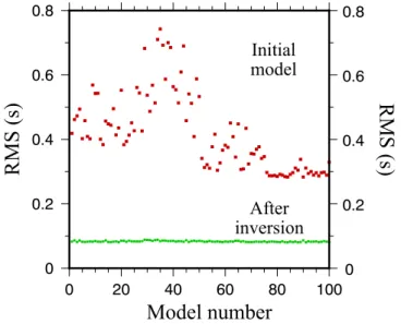
We used 100 different input models for the Monte Carlo inversion discussed in the manuscript. Figure A1 shows the RMS misfit for the starting model and the final misfit after inversion as described in the text, which is of the order 0.080–0.088 s for the inversion for crustal velocity structure and Moho depth using first breaks of crustal arrivals (Pg) and Moho wide-angle reflections (PmP). RMS, root mean square.

Figure A1. RMS difference between observed picked Pg and PmP arrival times and calculated times based on 100 random models, each of which was derived from assumptions of an plane layer and ±10% and

±6% variation in upper and lower P wave velocities. Red dots = initial model. Green dots = after inversion. Pg, crustal arrivals; PmP, Moho reflection.

Appendix B: Subsurface loads

In addition to using the present day bathymetry in the flexure calculations we also considered a load de- fined by the 6 km s⁻¹ refractor assuming that it was this load, rather than the present day bathymetry, that displaced water, flexed the crust and lithosphere and produced the free-air gravity anomaly observed today.

A difficulty in using such a subsurface load is that the refractor is only defined along a single seismic line.

When calculating the flexure due to the present day bathymetry we assumed a base for the load defined by the 5.26 km contour and so we used this same contour to estimate the spatial extent of the load associated with the 6 km s⁻¹ refractor, assigning it the mean depth of the refractor of 8.10 km rather than the mean depth of the present day bathymetry of 5.26 km. The load was then estimated by gridding the difference between the mean depth of 8.10 km and the depth to the 6 km s⁻¹ refractor along the seismic line and the associated flexure and gravity anomaly calculated assuming a load and infill density of 2,882 kg m^-3 and a range Tc and Te. The resulting load is shown in Figure B1, together with the flexure and gravity anomaly for assumed values of Tc = 5.1 and Te = 14 km.

Data Availability Statement

We are grateful to the officers, crew, scientific and technical staff onboard R/V Marcus G. Langseth and the OBS teams from GEOMAR and the Ocean Bottom Seismometer Instrument Center (OBSIC) at Woods Hole Oceanographic Institution for making the acquisition of the seismic and gravity data used in this paper possible and V. Cortes Rivas, W. Fortin, H. Harper, J. Leeburn, M. Liu and C.L. Nguyen for their help with OBS deployment/recovery and data editing at sea. We thank B. Tozer and D. Sandwell (Scripps Institute of Oceanography) and O. Andersen (Denmark National Space Institute) for making available the global SRTM15 + V2.0 bathymetry and DTU15 gravity fields respectively and W. Sager and A. Trehu for their helpful reviews. The figures in this paper were constructed using GMT (Wessel & Smith, 1991). The seismic, gravity and swath bathymetry data acquired during the MGL1902 cruise (doi: 10.7284/908198) will be made available through the Marine Geoscience Data System (https://www.marine-geo.org/tools/

entry/MGL1902) and PANGAEA (https://doi.pangaea.de/10.1594/PANGAEA.926068), the data publisher for Earth and Environmental science.

Figure B1. Plot of the load, flexure and gravity anomaly associated with the 6 km s⁻¹ iso-velocity contour.