1. Introduction
The lack of high-resolution bed topography and knowledge about the subglacial conditions in Greenland and Antarctica is one of the largest sources of uncertainty in present ice sheet projections (Morlighem et al., 2019) and higher resolution bed topography is needed to improve the accuracy of ice sheet models (Durand et al., 2011). The subglacial environment of the Antarctic and Greenland Ice Sheet (AIS, GrIS) is only poorly known from direct observations. The technical and logistical efforts for an analysis of the base underneath ice, often several kilometres thick, is much more challenging than observations on paleo-glaci- ated areas on land or the seafloor through remote sensing techniques (e.g., Clark and Meehan 2001; Stokes et al., 2013) or marine swath bathymetry (e.g., Arndt et al., 2020; Dowdeswell et al., 2004). Most of the knowledge about the ice covered bathymetry, bed topography and basal properties are deduced from the analysis and interpretation of indirect observations like radio-echo sounding (Fretwell et al., 2013; Hum- bert et al., 2018; Morlighem et al., 2019, 2017; Schroeder et al., 2019, 2020; Winter et al., 2017), seismic (Brisbourne et al., 2014; Dow et al., 2013; Hofstede et al., 2018; Kulessa et al., 2017; Rosier et al., 2018;
Smith et al., 2020) as well as magnetic and gravimetric surveys combined with modeling approaches (An et al., 2019; Cochran & Bell, 2012; Eisermann et al., 2020; Muto et al., 2013). In the central regions of the
Abstract
The ice stream geometry and large ice surface velocities at the onset region of the Northeast Greenland Ice Stream (NEGIS) are not yet well reproduced by ice sheet models. The quantification of basal sliding and a parametrization of basal conditions remains a major gap. In this study, we assess the basal conditions of the onset region of the NEGIS in a systematic analysis of airborne ultra-wideband radar data. We evaluate basal roughness and basal return echoes in the context of the current ice stream geometry and ice surface velocity. We observe a change from a smooth to a rougher bed where the ice stream widens, and a distinct roughness anisotropy, indicating a preferred orientation of subglacial structures. In the upstream region, the excess ice mass flux through the shear margins is evacuated by ice flow acceleration and along-flow stretching of the ice. At the downstream part, the generally rougher bed topography correlates with a decrease in flow acceleration and lateral variations in ice surface velocity.Together with basal water routing pathways, this hints to two different zones in this part of the NEGIS: the upstream region collecting water, with a reduced basal traction, and downstream, where the ice stream is slowing down and is widening on a rougher bed, with a distribution of basal water toward the shear margins. Our findings support the hypothesis that the NEGIS is strongly interconnected to the subglacial water system in its onset region, but also to the subglacial substrate and morphology.
Plain Language Summary
The Northeast Greenland Ice Stream (NEGIS) transports a large amount of ice mass from the interior of the Greenland Ice Sheet (GrIS) toward the ocean. The extent and geometry of the NEGIS are difficult to reproduce in current ice sheet models because many boundary conditions, such as the properties of the ice base, are not well known. In this study, we present new characteristics of the ice base from the onset region of the NEGIS derived by airborne radio-echo sounding data. Our data yield a smooth and increasingly lubricated bed in the upstream part of our survey area, which enables the ice to accelerate. Our results confirm the hypothesis that the position of the ice stream boundaries are coupled to the subglacial hydrology system.© 2020. The Authors.
This is an open access article under the terms of the Creative Commons Attribution License, which permits use, distribution and reproduction in any medium, provided the original work is properly cited.
Steven Franke1 , Daniela Jansen1 , Sebastian Beyer1,2 , Niklas Neckel1 , Tobias Binder1,† , John Paden3 , and Olaf Eisen1,4
1Alfred Wegener Institute, Helmholtz Centre for Polar and Marine Research, Bremerhaven, Germany, 2MARUM - Center for Marine Environmental Sciences, University of Bremen, Bremen, Germany, 3Center for Remote Sensing of Ice Sheets (CReSIS), University of Kansas, Lawrence, KS, USA, 4Department of Geosciences, University of Bremen, Bremen, Germany
Key Points:
• Basal roughness at the onset of the NEGIS hints to a geomorphic anisotropy and a change in the geomorphological regime
• Basal water is funneled into the ice stream upstream and redistributed toward the shear margins further downstream
• A smooth and progressively lubricated bed reduces basal traction and favors the acceleration of the NEGIS at its onset
Correspondence to:
S. Franke,
steven.franke@awi.de
Citation:
Franke, S., Jansen, D., Beyer, S., Neckel, N., Binder, T., Paden, J., & Eisen, O.
(2021). Complex basal conditions and their influence on ice flow at the onset of the Northeast Greenland Ice Stream.
Journal of Geophysical Research: Earth Surface, 126, e2020JF005689. https://
doi.org/10.1029/2020JF005689 Received 14 MAY 2020 Accepted 8 DEC 2020
†Now at Ibeo Automotive Systems, Ham- burg, Germany
AIS and GrIS, little is known about the distribution and properties of bedrock, lithified and unlithified sediments, liquid water quantity, hydromechanical processes and the thermal and mechanical properties of ice (Clarke, 2005). Variations of these parameters over time can influence the spatial and temporal behav- ior of the ice sheets and their streams, by altering the fast flow dynamics or the mobilization of subglacial sediments. It is assumed that parts of the base of the GrIS are covered by mechanically weak sediments, which facilitate basal sliding (Christianson et al., 2014; C. F. Dow et al., 2013). Furthermore, an analysis of the thermal state of the base reveals large areas of a thawed bed and high melt rates at the interior of the GrIS (Fahnestock, 2001; Jordan et al., 2018; MacGregor et al., 2016). However, the response of changes at the glacier base to the ice surface dynamics can vary on several time scales (Ryser et al., 2014).
In Greenland, one feature causing the most significant discrepancies between numerically modeled and observed ice surface velocities is the Northeast Greenland Ice Stream (NEGIS) (Aschwanden et al., 2016), which therefore represents one of the largest uncertainties for ice flow predictions. Several studies assessed the genesis as well as the positioning and geometry of the NEGIS in its onset region close to the ice di- vide (Fahnestock, 2001; Fahnestock et al., 1993; Joughin et al., 2001). The ice stream is constrained by its 400-km-long shear margins, and their locations at its onset region show no apparent indications for a topographic control (Franke et al., 2020b; Holschuh et al., 2019). Christianson et al. (2014) established an extended hypothesis on the initiation and development of the NEGIS based on these studies and an analysis of data from an extensive geophysical survey at the onset of the ice stream, centered at the drill site of the EGRIP ice core where the ice stream widens (Vallelonga et al., 2014). The ice stream is most likely initiated by anomalous high geothermal heat flux (GHF) close to the ice divide (Fahnestock, 2001). The GHF is the primary control on the generation of basal meltwater and the sensitivity of the hydrology system (Smith- Johnsen et al., 2020). In the absence of cross-marginal ice flow, acceleration along the trunk of NEGIS should lead to the development of a surface trough. However, the lack of an observed trough must mean acceleration is compensated by an influx of ice through the shear margins (Christianson et al., 2014). The increasing ice flow velocity of the onset of the NEGIS in its current geometry would lead to the development a surface trough, which is not consistent with observations.
In present ice-sheet models, the NEGIS is reproduced through estimating basal-shear stress from inverse methods informed by surface velocities (Larour et al., 2014; Smith-Johnsen et al., 2019). Estimates of basal resistance are not accurate enough to sufficiently reproduce geometry and surface velocities of ice streams by ice-flow models, as our understanding of processes and conditions is still very limited. In this regard, the analysis of the basal roughness has become important for glacial geomorphological research and is an increasingly accepted attribute to describe subglacial conditions and to derive a controlling factor for the dynamics of ice-sheets (Smith et al., 2013). Basal roughness parameters can thus help us to discriminate whether the ice is underlain by softer sediments or harder rock, to reveal traces of former ice dynamics, to constrain the thermal regime and identify potential processes of subglacial erosion and deposition of sedi- ments (Bingham & Siegert, 2009). They are key parameters for the ice—bed coupling (Hughes et al., 2011), to model basal sliding (Wilkens et al., 2015) as well as a parameter for subglacial hydrology studies (Meyer et al., 2018). At present, the roughness of the bed topography is typically analyzed by spectral analysis of vertical and horizontal topography variations, based on the approaches of Shepard et al. (2001), Taylor et al. (2004), and Li et al. (2010). In many studies, basal roughness shows a clear correlation to basal drag and ice sheet velocity (Smith et al., 2013). In radio-echo sounding measurements, the roughness of the subglacial topography on different scales also influences the scattering of reflected radar waves (Jordan et al., 2017) and, thus, the reflectivity of the bed (Jacobel et al., 2010). Furthermore, the intensity and reflec- tion pattern of the bed return informs us about the reflection properties of the base, thus complementing inferences made by the roughness parameter. Jordan et al. (2017), for example, analyze the radar scatter- ing in combination with the topographically derived roughness to evaluate the relationship between basal roughness and the basal thermal state. The study concludes that frozen regions are relatively smooth and many thawed regions are relatively rough.
The majority of subglacial roughness studies in Antarctica focus on outlet glaciers (Bingham & Siegert, 2007, 2009; Diez et al., 2018; MacGregor et al., 2013; Rippin et al., 2011, 2014, 2006; Taylor et al., 2004) with only a few studies extending over large areas (e.g., Eisen et al. [2020] in East Antarctica). In a study to model the surface flow field of Pine Island Glacier, Wilkens et al. (2015) related basal sliding to a bed roughness
parameter and were able to reproduce some essential flow features, like the location of the fast-flowing cen- tral stream and various tributaries. One of the first studies of basal roughness in Greenland was conducted by Layberry and Bamber (2001) using the residual bed elevation deviation to quantify basal roughness. An estimate of the basal roughness distribution based on a spectral approach for those part of GrIS covered by radio-echo sounding data was given by Rippin (2013). A recent study by Cooper et al. (2019) indicates dif- ferent relationships between ice flow and basal roughness parameters. They conclude that in certain regions of slow ice flow, coinciding with low vertical roughness (i.e. smooth topography), a mechanism other than basal sliding must control ice flow. The relation between basal traction and sliding is still under debate and varies for different glaciological settings. For example, the study of L. A. Stearns and van der Veen (2018), observed that bed friction, which should control basal sliding, does not control the rapid flow of a large number of glaciers in Greenland. For a full account of the discussion also see the subsequent replies to the study (Minchew et al., 2019; Stearns & van der Veen, 2019). Furthermore, the inverse correlation between basal roughness and ice-sheet flow velocity (slow-flowing areas are mostly smooth, while increased ice flow shows rougher beds) encouraged the authors of more recent studies to rethink the influence of basal rough- ness to basal traction (Rippin, 2013). Possible mechanisms that control basal traction could be the thermal state at the base, subglacial hydrology and the rates of erosion and deformation of sediments.
In this paper, we use airborne radar data from AWI's ultra-wideband radar system to analyze the basal conditions of the onset of the NEGIS. We perform a spectral roughness analysis to characterize the pattern of the bed return signals and investigate the subglacial roughness parallel and perpendicular to ice flow.
For the basal roughness analysis on finer spatial scales, we analyze the scattering pattern of the bed return echoes. Based on an improved bed elevation model, we investigate subglacial water pathways. We then com- bine these data with an analysis of ice mass flux at the ice stream. This should ultimately give a consistent picture of the processes at the base, which control ice flow dynamics. Finally, we use our larger-scale data set to discuss the extended hypothesis of Christianson et al. (2014) of the initiation and development of the NEGIS as well as the positioning of the shear margins in its onset region.
Our results reveal a regional change in basal roughness and the pattern and intensity of the basal return echo from the upstream toward the downstream part in our study area on the NEGIS (Figure 2). Further- more, we detect a bed roughness anisotropy concerning the ice flow direction, indicating streamlining par- allel to ice flow. The analysis of water flow paths on the basis of a better resolved bed topography confirms the hypothesis that the subglacial hydrology and the position of the shear margins are tightly coupled.
2. Data and Methods
2.1. Survey Area and Data Acquisition
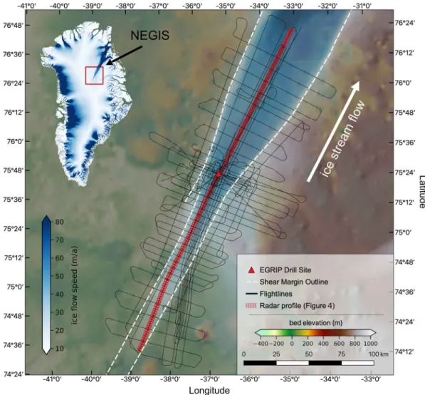
We use airborne radar data of the EGRIP-NOR-2018 survey in the onset area of the NEGIS (Figure 1). The data were collected with the AWI multi-channel ultra-wideband (UWB) airborne radar sounder (for details see Arnold et al., 2019; Franke et al., 2020b; Hale et al., 2016) and recorded at a center frequency of 195 MHz and a bandwidth of 30 MHz. The transmit signals are chirp waveforms transmitted at three stages with different pulse durations and gains to obtain high signal-to-noize ratio (SNR) in all parts of the radargrams.
Radar data processing comprises pulse compression, along-track SAR processing (fk-migration) and cross- track array processing. A complete methodological description of the radar data processing and uncertainty estimation is described in Franke et al. (2020b). In the study area, the NEGIS accelerates from ∼ 10–80 m/a over a distance of roughly 300 km and widens from ∼ 20 km in the upstream boundary of our survey area to
∼ 65 km further downstream (Figure 1). More than 8,000 km of survey profiles are distributed over an area of more than 250 km along ice flow direction and 50–100 km across, covering the interior of the ice stream, the shear margins and the slow-flowing area in the vicinity of the NEGIS (Figure 1). The profile spacing of across-flow profiles is 5 km in the central part of the survey area, near the drill site of the East Greenland Ice-core Project (EGRIP; http://eastgrip.org), and 10 km further upstream and downstream. Along-flow profiles are mostly aligned along calculated pathways of ice flow based on the velocity field of Joughin et al. (2017). For the rest of this paper, we will refer to upstream and downstream as the regions upstream and downstream of the EGRIP drill site, respectively.
2.2. Basal Roughness Calculation
We define basal roughness as the relative vertical and horizontal variation of the topography of the ice-bed interface. In our analysis we calculate two parameters (ξ and η), which are commonly used to characterize basal roughness (Cooper et al., 2019; Gudlaugsson et al., 2013; Li et al., 2010; Rippin et al., 2014):
1. ξ reflects the vertical irregularity of the bed and provides information about the dominating vertical amplitudes. This roughness parameter is defined as the integral of the wavenumber spectrum over the range of a moving window (MW). Values close to 0 reflect the dominance of smaller amplitudes and a smoother topography.
2. Li et al. (2010) introduced the frequency roughness parameter η, which is calculated by dividing the vertical roughness ξ by the roughness of the bed slope ξsl. This parameter reflects the horizontal variation pointing out the dominance of a particular wavelength. High values represent the dominance of longer wavelength and smaller values the dominance of shorter wavelength.
Figure 1. Overview of the survey area in the interior of the Greenland Ice Sheet at the onset of fast flow of the NEGIS.
The black lines, which are centered at the EGRIP drill site, represent the survey profiles of the EGRIP-NOR-2018 airborne UWB radar survey (Franke et al., 2020b). The white dashed lines show the outline of the shear margins (determined from satellite imagery) and the dashed red line the radar profile shown in Figure 4. Bed elevation is referenced to mean sea level (EIGEN-6C4 geoid (Förste et al., 2007), this reference applies to all other maps showing the bed elevation) and ice flow velocity is based on the data set of Joughin et al. (2017) and is shown in blue color code for velocities larger than 10 m/a. The projection of this map and all following maps are shown in the coordinate system EPSG 3413 (WGS84/NSIDC Sea Ice Polar Stereographic North).
Figure 2. Survey area at the NEGIS showing (a) along- and (c) across-flow profiles of the vertical roughness parameter ξ and the horizontal roughness parameter η in (b) along and (d) across-flow profiles respectively. Both parameters are shown on a logarithmic scale. The background map represents the EGRIP-NOR-2018 bed topography of Franke et al. (2020b) in meters, referenced to mean sea-level (EIGEN-6C4 geoid). Histograms a’ and b’ show the distribution of ξ and η for the along-flow profiles for the upstream and downstream region, respectively (orange and blue outline in a and b). The y-axis on the histograms represents the kernel density estimation. The distribution of η in the western and eastern part of the downstream region (red and black outline in d) are shown in a histogram d’.
We use the bed picks of the EGRIP-NOR-18 data set (Franke et al., 2019, 2020b) for basal roughness calcu- lation. The roughness analysis in this paper is based on the approaches of Hubbard et al. (2000) and Taylor et al. (2004) and uses a Fast Fourier Transform (FFT) to analyze the wavenumber spectra of variations in topography (Gudlaugsson et al., 2013). This requires a uniform sampling interval of data points on the bed elevation profiles. Synthetic Aperture Radar processing of our radar data already includes the creation of a new coordinate system with a constant spatial sampling interval for the focused radar data. The average spacing between data points is 14.78 m. For each data point on a linearly detrended profile, we calculate the wavenumber spectrum over a MW of 2N data points. We test two different MW for our analysis: (i)
∼ 400 m, which corresponds to 32 data points (N = 5) and (ii) ∼ 2,000 m, which corresponds to 128 data points (N = 7). For the 32-data point MW, one data point covers the roughness at a resolution which is finer than the cell size of 500 m used for the bed elevation data sets of Morlighem et al. (2017) for Greenland and the NEGIS onset region by Franke et al. (2020b). To make sure that this small MW does not suppress long- wave structures, we compared the result of the 500 m MW with the results obtained for the ∼ 2,000 m MW.
The comparison shows that significant changes are represented in both MWs. Because we focus on regions where clusters of high or low roughness values or trends appear, we use the larger (N = 7) MW for further analysis. For this manuscript, we will refer to this kind of basal roughness as large-scale roughness.
Because the interpretation of roughness parameters is highly directionally dependent and the dominating factor influencing bed formations is the direction of ice flow as shown by Falcini et al. (2018), Gudlaugsson et al. (2013), and Rippin et al. (2014), we separately analyze along- and across-flow profiles. We present roughness values on a logarithmic scale to emphasize the range of up to four orders of magnitude.
2.3. Ice Mass Flux
In order to calculate the ice mass flux in the survey area we employed 20 flux gates orientated perpendicular to the ice flow direction. These are limited by 19 additional flux gates along each shear margin forming 19 closed boxes. Following Neckel et al. (2012) the ice flux through each gate is calculated by
1
2 ( )
i N
i i i i
F i v H d
(1) with N being the number of pixels in the flux gate and ϕ′i the normal angle to the flux gate at position i.
The ice flow velocity, ice thickness and pixel spacing are indicated by vi, Hi, and di, respectively. In order to translate volume flux into mass flux, we employed an ice density of 910 kg m−3.
We consider the full ice column for the analysis of the flux gate balance and calculate the ice fluxes as if there is no basal drag (plug flow). As input data, we use the ice surface velocity data from Joughin et al. (2017) and the ice thickness data from Franke et al. (2020b). Because we make only a large-scale interpretation of the mass flux in our survey region, we neglect surface and basal mass balance.
2.4. Basal Return Power
We use the intensity of the return echoes from the basal interface as an additional parameter to analyze the basal conditions at the onset region of the NEGS. We follow the approach of Jordan et al. (2016) and Jordan et al. (2017), which is based on the method developed by Oswald and Gogineni (2008) and Oswald and Gogineni (2012). The return power is calculated from an along-track average of the basal return echo and is defined as the integral over a window of samples that represent the reflected energy from the bed (Equation 2). Before arithmetically averaging along-track, we use the bed picks of Franke et al. (2020b) to shift the bed reflection to a single level. The arithmetical averages are phase-incoherent, but help to reduce fading effects and to smooth power fluctuations (Oswald & Gogineni, 2008). We tested different values for along-track averaging and chose a value of 50 (two times 25 adjacent traces). With this value the power fluctuations are small enough to analyze as many tracks as possible, but also not too low, so that the signal is not smoothed too much. The size of the range window is kept variable and is set for a threshold above 3.5% the noise floor for a section above the bed reflection. The upper boundary is defined where the signal starts to be above the threshold and the lower boundary where the signal drops for the first time below this
threshold (for further details, see Figure 3 in Jordan et al., 2016). We follow Jordan et al. (2016) and define the integrated power Pint, referred to as the bed return power (BRP), by
Llower ( ),
int Lupper i
P P L
(2) with the upper and lower limit of the integration window threshold Lupper and Llower, the return power of a sample P and the depth range index Li. The full waveform of the basal return in the integration window rep- resents an overlay of the specularly reflected energy from nadir and scattered energy from along- and cross- track off-nadir (Young et al., 2016). The majority of the scatter from off-nadir will arise from across-track re- flections because SAR post-processing reduces the footprint of return signals in along-track (Raney, 1998).
Similar to the approaches of Jordan et al. (2016) and Jordan et al. (2018), we implement additional quality control rules. Traces where the window for the integration of depth-range bins was smaller than five range bins were abnormally thin and abrupt reflections associated with clutter and were removed. The maximum size of the integration window is set to 40 range bins to limit the amount of far off-nadir layover signals.
The radar wave bed return power is corrected for spherical spreading and therefore depends mainly on the properties of the ice-bed interface, scattering properties of the bed, anisotropy in the ice fabric and dielec- tric attenuation within the ice column. The largest energy loss is related to dielectric attenuation, which depends on ice temperature, chemistry and other impurities in the ice column (Corr et al., 1993; Matsuo- ka, 2011). If dielectric attenuation varies significantly, the distinction between basal water and dry sediment is difficult because the effect of englacial attenuation can be much more significant than the contrast in reflectivity between a wet and dry base (Matsuoka, 2011).
No ice sheet models exist so far to accurately reproduce ice flow and englacial temperature in the rather complicated region of the NEGIS ice stream with its distinct shear margins. Therefore, we apply a simple linear fit between bed power and ice thickness to obtain the average attenuation rate. Based on this fit, we correct for englacial attenuation with a constant value of 8 dB per km ice thickness. However, this correc- tion will only remove the depth-correlated component of the bed reflection power.
The correction factor depends mainly on ice temperature, which in turn depends on the geothermal heat flux (GHF), the mean annual air temperature, surface accumulation rates and frictional heating at the gla- cier bed and from internal ice deformation. Estimates on GHF vary significantly and are associated with large uncertainties (Rogozhina et al., 2012). Other radar studies investigating BRP at the NEGIS find differ- ent values to correct for englacial attenuation. Christianson et al. (2014) found attenuation rates from a lin- ear fit between bed power and ice thickness at the onset of the NEGIS of 8 dB/km. Attenuation rates at the NEGIS onset in the Greenland wide study of (Macgregor et al., 2015) are larger than 12 dB/km, but show an increasing uncertainty toward the ice sheet margin. The overall resulting depth-averaged attenuation rate of the common midpoint survey of Holschuh et al. (2016) are up to 3 times higher (27 db/km) than the attenuation rates found in the previous studies.
2.5. Waveform Abruptness
The intensity of the integrated bed return echo as well as the length of the integration window is sensitive to small-scale variations in basal roughness (Cooper et al., 2019), which are not resolved in the radar measure- ments and depend on the size of the Fresnel zone. The diameter of the Fresnel Zone for a bandwidth of 180–
210 MHz and an ice thickness range of 2–3 km is ∼ 60 m. Ice-bed interface roughness and the wavelength of the radar signal determines the nature of the electromagnetic scattering. However, rough subglacial terrain can produce side reflections, which are difficult to separate from the nadir bed echo return. In this case, the footprint of the radar signal and consequently the area of the basal backscatter is larger than the Fresnel zone and determined by the beam angle of the transmitted signal. To characterize the basal scattering, we follow the approach of Oswald and Gogineni (2008) which has been adapted and extensively used in Green- land by Cooper et al. (2019), Jordan et al. (2016, 2017), and Jordan et al. (2018) analyzing the waveform abruptness of the bed reflection. We follow Cooper et al. (2019) and define the abruptness parameter A by
max
agg, A P
(3)P
where Pmax is the maximum amplitude of the basal return echo in the integration window and Pagg the integrated basal return power (Oswald and Gogineni, 2008). A large Pmax in a small integration window will result in a large value of A. If the reflected energy is distributed over a larger integration window, it Figure 3. Flux gate analysis of the onset of the NEGIS. Panel (a) shows the position of central flux gates (red) and flux gates at the shear margins (yellow and orange, respectively). The location where the ice stream widens is marked with a white outline. Panel (b) shows the mass flux (in Gt/yr) through the central gates (Qout; red line) in comparison to the sum of the respective upstream central gate (Qup) and the corresponding shear margin gates (Qsouth + Qnorth; black dashed line). The blue line represents the width of the central gates. The cumulative mass flux through the northern and southern shear margin (as well as the sum of both) is shown in panel (c).
will decrease the maximum amplitude and result in a small value of A (for details see Figure 4 in Cooper et al., 2019). High values indicate an abrupt return (i.e., along-track focusing was sufficient to recover ener- gy to the nadir reflection point), whereas low values indicate a broad return (likely due to energy recovered from a range of cross-track angles, which could not be focused due to the narrow antenna array in the cross-track direction). We will refer to this scattering-derived roughness as small-scale roughness because it represents roughness of a different scale and type than the spectral large-scale roughness.
2.6. Basal Water Routing
We compute (potential) subglacial water pathways from the hydrological potential F. We assume that the water flow depends on the elevation potential and the water pressure rw (Shreve, 1972). Under the assump- tion of equilibrium between water pressure and ice overburden pressure we can write
Φ wgb igH,
(4) where ρw is the density of water, g is the acceleration due to gravity, b is the bed elevation, and H the ice thickness (Le Brocq et al., 2009; Livingstone et al., 2013). We apply a simple flux routing scheme as described by Le Brocq et al. (2006) to successively compute the number of upstream cells (cells that po- tentially contribute water to this cell) for each grid cell. The equilibrium assumption in Equation 4 is only valid at large scales (km) and makes the potential especially sensitive to the ice surface gradient. Hence, this method cannot account for localized water flow, such as flow through channels (more details on our implementation can be found in Calov et al., 2018). We make use of bed topography and ice thickness data of the EGRIP-NOR-2018 bed elevation model from Franke et al. (2020b) as well as the BedMachine v3 to- pography (Morlighem et al., 2017; BMv3). We use both models as input fields to analyze the sensitivity of subglacial water routing to the bed topography. While this method allows for using basal melt rates as input to quantify transported water volumes, we chose to simply count the number of upstream cells as a measure for potential water pathways. Basal melt rates are poorly constrained for this area, in particular, because the spatial variations in geothermal heat flux are subject to considerable uncertainties (Dow et al., 2018;
Jordan et al., 2018; Smith-Johnsen et al., 2019). Nevertheless, we can use the water pathways to estimate the distribution of basal water, particularly for areas where we can infer a thawed base and the generation of meltwater by other methods. Several studies have detected or modeled water at the base of the Greenland Ice Sheet, but the amount of basal water is uncertain and difficult to measure (Fahnestock, 2001; Jordan et al., 2018; MacGregor et al., 2016).
3. Results
3.1. Spatial Distribution of Spectral Basal Roughness
We analyzed ∼ 370,000 data points for vertical and horizontal roughness with a spectral analysis approach and present our result as the dominating vertical amplitude (ξ) and horizontal wavelength (η) over a 2,000 m MW in along-flow and across-flow profiles in Figure 2. We observe that high ξ, in general, correlate with higher η values. Also, the correlation of ξ and η shows higher vertical roughness values for the same hori- zontal roughness in cross-flow profiles compared to along-flow profiles. On the linear scale, vertical rough- ness values vary on the order of four magnitudes and horizontal roughness in the order of 2.5. Basal rough- ness values show distinctly different spatial patterns, independent of flight-line orientation, in two areas:
upstream and downstream of the EGRIP drill site (Figure 2). We will refer to these two regions as Rup
(upstream) and Rdown (downstream), respectively, and will present their particular characteristics in the following.
Region Rup shows low vertical and horizontal roughness values for profiles along- and across-flow. On av- erage, ξ and η are small for profiles along-flow in the ice stream, while we observe an increase of ξ for pro- files perpendicular to flow when moving from the upstream end in the south-west toward the EGRIP drill site. Across-flow profiles show distinctly different roughness values within and outside of the ice stream.
Outside of the south-eastern shear margin, η is higher than inside the ice stream. Along-flow profiles that
are located outside of the ice stream show similar horizontal and vertical roughness values as along-flow profiles in the ice stream. The statistical distribution of roughness values for both, ξ and η, for across-flow profiles is much wider. However, it has to be noted that the profiles also extend further to the South-East and North-West here than further upstream.
The bed elevation in the transition area rises about 500 m in flow direction and the average ice thickness decreases 400 m compared to the region Rup. The transition zone between regions Rup and Rdown is charac- terized by a dominance of lower vertical amplitudes (ξ) and shorter horizontal wavelengths (η). Both the vertical and horizontal roughness values are, on average, higher for along and across flow profiles in the downstream region Rdown in comparison to the upstream region Rup. Along-flow profiles show a strong increase in ξ and η, and both remain high in value with little variability. Along profiles perpendicular to ice flow, ξ shows a trend toward increasing values downstream and at the upstream end of region Rdown. The horizontal roughness η shows two different domains for across-flow profiles. Low values of horizontal roughness dominate in the south-eastern part of region Rdown, which we will refer to as region Reast, and high values in the north-western region Rwest (Figure 2d). The transition from high to low values between these two sub-regions, which we will refer to as Rtrough (Figure 2c), coincides with the steep eastern flank of a central ridge as well as with a local topographic low (Franke et al., 2020b). In the region Rtrough we observe low vertical roughness values in the center and higher roughness values at the edges of the region. For re- gion Rdown, along-flow profiles located outside of the ice stream, show a similar development in both, ξ and η (Figures 2a and 2b). For the parts of across-flow profiles, which are located outside of the shear margin, we detect the same trend of increasing vertical roughness from upstream to downstream (Figure 2c), but not in the horizontal roughness which is highly variable on across-flow profiles outside the shear margins.
3.2. Development of Ice Stream Flux in a Kinematic-Geometrical Context
For an interpretation of subglacial properties and ice stream development, we consider a flux balance, a development of englacial units along ice flow and the change of width and lateral surface velocity along the ice stream.
The flux gate analysis focuses on (i) the comparison of the mass flux though a central gate (Qout) to the sum of mass flux of the upstream gate and the respective shear margin gates (Qup + Qsouth + Qnorth; shown sche- matically in Figure 3 b/c) as well as (ii) the cumulative mass flux through the shear margins, which shows the following features:
1. Upstream of the EGRIP drill site (gates 1–8) the ice stream has a constant width and ice mass flux increases and we observe an acceleration of the ice surface speed. The initial mass flux at gate one is relatively small and Figure 3c indicates that most of the additional mass flux is provided through the southern shear margin.
2. Between gates 8 and 15, the ice stream widens. Total mass flux increases constantly, with a small step due to the shift northward of the northern shear margin. The widths of the central gates increase, and thus, provides the ice stream with additional mass flux through the shear margins.
3. After gate 15, the widening rate of the ice stream decreases but the flux gates indicate no change in mass flux.
We use two isochrones in a central radar profile as boundaries to define two englacial units. Figure 4a shows this radar profile, which is oriented along-flow at the location indicated in Figures 1 and 5 with a red line.
This radar section is composed of two profiles and was concatenated at the location of the EGRIP drill site.
The profile from 0 to 160 km will be referred to as the upstream section and the profile from 160 to 280 km as the downstream section. There is an offset between the two profiles of 1 km across-flow. For both sections, we tracked two internal reflection horizons, which have a respective age of ∼ 30 and 52 ka, respectively, which we transferred from dating of radar reflections at the location of the NGRIP ice core (Vallelonga et al., 2014). We will refer to the thickness of these two layers as the basal unit between the 52 ka horizon and the bed reflection; and the internal unit between the 30 ka horizon and the 52 ka horizon, respectively.
The upstream section shows an increase of ice surface velocity (Figure 4b) from 12 to 58 m/a over a distance of 150 km. Vertical and horizontal roughness (Figures 4c and 4d) are on average low but vary over two to three orders of magnitude. Furthermore, the thickness of the internal and basal unit remains nearly con-
stant in the upstream section (Figure 4e). In the downstream section, between 150 and 175 km, we observe a decrease of the internal unit thickness of ∼ 125 m, whereas the basal unit thickness remains constant down- stream to 240 km. The surface velocity in the downstream section shows a small decrease between 175 and 210 km and increases thereafter to ∼ 80 m/a. Vertical and horizontal roughness in the downstream section is higher on average than in the upstream section. The increase in roughness correlates with a decrease in ice surface velocity and also with a decrease in the thickness of the ice column. The internal unit becomes thinner while the thickness of the basal unit remains constant.
Figure 5 shows the downstream section and the spatial distribution of ice surface velocity, flow lines indi- cating the flow path (Figure 5a) of a point on the ice surface, as well as vertical and horizontal roughness (Figures 5b and 5c respectively). Surface flow velocity is about 5–8 m/a higher in the eastern part of the section than in the western part. The area of increased ice surface velocity correlates with the location of Figure 4. Evolution of several basal and englacial properties in ice flow direction, extending from far upstream to the downstream end of our survey area (red line in Figures 1 and 5). Because there is no continuous survey profile, the downstream part (right part of the dashed line) is offset ∼ 1 km to the South-East (transverse to along-flow profile orientation) relative to the upstream profile (left of the dashed line). The transition between the two profiles marks the position of the EGRIP drill site (yellow triangle). Ice flow direction is from left to right. (a) along-flow radargrams with continuously tracked surface, two internal ice units (basal unit in purple and internal unit in green) and bed reflection; (b) ice surface flow velocity; (c) horizontal roughness η and (d) vertical roughness ξ, both with the same color code and scaling as in Figure 2; and (e) the thickness of the internal and basal unit.
the basal topographic depression (Rtrough) and is also characterized by lower vertical and horizontal rough- ness. Flowlines in Figure 5a show that ice surface flow in the eastern part of the region (yellow flow line in Figure 5a) deviates slightly toward south-east (orographic right) as it flows around the central ridge trough the topographic depression, whereas a flowline located north-west to the ridge bend less toward the trough (green flow line in Figure 5a).
3.3. Basal Return Power and Waveform Abruptness
In Figure 6, we present the BRP of the basal reflection in (dB) for profiles aligned along-flow (a) and across- flow (b). The BRP, which is corrected for spherical spreading and englacial attenuation (constant value of 8 dB per km ice thickness), varies in a range of −25 to 25 dB. The BRP for the area around the EGRIP drill site agrees with the data of Christianson et al. (2014) and Holschuh et al. (2019). These two studies analyz- ed the BRP in the immediate surrounding of the EGRIP drill site, which they characterized as high return power in the center of the ice stream, low return power in the area of the shear margins and again higher return power outside of the shear margins. In general, the BRP on along- and across-flow profiles within the ice stream is higher than outside. Highest BRP values on across-flow profiles are concentrated within a ∼ 10 km corridor in the center of the ice stream, and decrease toward the shear margins. Along-flow profiles in the upstream part, which are located inside of the ice stream, show a stronger BRP than profiles located outside of the ice stream. Downstream of the EGRIP drill site, where the ice stream is widening, high return power values of across-flow profiles are not constrained to the center of the ice stream. Further downstream, BRP in across-flow profiles is highest in the region of the topographic depression (Rtrough), is lower on the central ridge and decreases toward the margins. The strongest drop of BRP in profiles parallel to flow profiles coincides with the location of the central ridge (ridge indicated in Figure 5a). However, be- Figure 5. Bed and flow properties in the downstream survey region, North-East of the EGRIP drill site (red triangle). Panel a shows the bed topography and flowlines of the ice surface (ice flow direction is toward North-East as indicated in Figure 1). Panel b shows the vertical roughness parameter ξ as well as the ice surface velocity (Joughin et al., 2017) in a range of 54–64 m/a (velocity values lower than 54 m/a are transparent). Panel c shows the same velocity map together with the horizontal roughness η. Both roughness maps (b and c) show the hillshade of the bed elevation in the background. The red line on all three maps represents the location of the radar profile in Figure 4.
Figure 6. Bed echo characteristics for (a) and (b) basal return power and (c) and (d) waveform abruptness for profiles oriented along-flow (a) and (c) and across-flow (b) and (d), respectively. Basal return power is corrected for spherical spreading as well as englacial attenuation losses (8 dB/km ice thickness) and displayed in decibel (dB with respect to unity). Waveform abruptness is expressed as the ratio between the maximum BRP and the integrated bed return power and is thus unitless. High values (yellow) represent the dominance of specular reflection and low values (dark purple) the dominance of diffuse scattering of the base. The yellow and blue rectangular outlines indicate the position of the radargrams in Figure 7. The interpretation of bed permittivity from the BRP data presented here is limited due to the simple correction scheme for englacial attenuation applied here. A large part of the spatial heterogeneity in BRP probably results due to an inaccurate englacial attenuation correction, which cannot be overcome due to an uncertainty in englacial temperature distribution.
cause we use a constant correction factor for englacial attenuation, some of the variations in BRP might be introduced by this correction. It is very likely that the large heterogeneity in BRP is a result from this simple correction scheme.
Figures 6c and 6d show the spatial distribution of the waveform abruptness for along- and across-flow profiles, respectively. Abruptness values range from 0.03 to 0.6, where smaller values are associated with a dominance of diffuse scattering (e.g., off-nadir reflections from cross-track) and higher values with more specular reflections. Along-flow profiles show significantly lower average abruptness values than profiles oriented perpendicular to ice flow in both, the upstream and downstream region. Fur- thermore, along-flow profiles in the upstream region show slightly higher abruptness values than the downstream region. Across-flow profiles in Figure 6d show the highest values in the upstream survey area, which are concentrated in the center of the ice stream. This patch of high abruptness values has a similar extent as the patch of high basal return power in Figure 6b. Lower abruptness values in the upstream area are aligned in a zone extending 2–5 km from the shear margin to the ice stream center and outside of the shear margins. In the downstream area, high abruptness values are located in a zone of a localized topographic depression (Rtrough) as well as in the immediate surrounding of the EGRIP drill site. Abruptness values in the downstream region, outside of these two areas are significantly lower. Values of BRP and waveform abruptness show a strong correlation in across-flow profiles but not as clear in along-flow profiles (high abruptness values with high BRP and low abruptness values with low BRP).
Two representative radargrams for the upstream and downstream region with their corresponding bed re- turn power and abruptness are shown in Figure 7. Profile 7a shows high bed return power and high abrupt- ness in the center of the ice stream (outlined with the black dashed line) and outside of the ice stream close to the shear margin (white and gray dashed line). The along-flow profile 7b in the center of the stream shows on average a constant high basal return power. Its waveform abruptness is on average higher between 0 and 12 km along-track and decreases thereafter. This change correlates with a step in the bed elevation, which marks a general change of the topographic regime.
3.4. Basal Water Routing
The subglacial water flux follows the gradient of the hydraulic potential. The direction of the water path- ways is in general oriented toward the direction of ice flow and decreasing ice thickness (Figure 8). We compared subglacial water routing derived by the EGRIP-NOR-2018 bed elevation model and the BMv3 bed elevation model (blue and red lines in Figure 8, respectively). The general pattern is the same: In the upstream region, pathways that drain the largest area lead into the ice stream and flow around bed obstacles. About 20 km upstream of the EGRIP drill site, the main water pathways lead through the shear margins into the ice stream toward the point of lowest bed elevation. The pathway with the highest number of upstream routing cells is entering the ice stream from the South-East. About 10 km upstream of the EGRIP drill site the routing inside of the ice stream follows the south-eastern shear margin and propagates downstream. Pathways entering the ice stream at the north-western shear margin propagate along the shear margin downstream. At the location of the drill site, the ice stream widens from ∼ 25 to
∼ 60 km at the downstream end of our survey area and two dominant pathways develop in the ice stream:
One on the south-eastern side of the ice stream with a higher number of upstream cells, and a second on the western side of the NEGIS. About 40 km downstream of EGRIP, the south-eastern path changes its location from the eastern shear margin to the local trough (our subregion Rtrough), continuing in ice-flow direction and then switching its location back to the shear margin after another 40 km. The north-west- ern pathway stays more or less in the area of the shear margin. Summarizing, the water routing in the downstream area seems to predominantly follow the location of the shear margins and local troughs in the bed topography in the ice stream.
We identify three locations where the routing pathways deviate significantly for the two topographies (fea- tures 1–3 in Figure 8). At all three features, the blue EGRIP-NOR-2018 water routing follows preferably the location of the shear margin outline, whereas the BMv3 routing deviates and flows toward the center of the ice stream.
4. Discussion
The analysis and interpretation of the conditions of the ice base inferred by airborne radar sounding data are subject to several uncertainties resulting from radar data processing, the energy loss in the ice column as well as the interpretation of basal roughness parameters. We address these uncertainties in detail in the appendix. The uncertainties from each method affects the robustness of our interpretations with different significance. For example, the potential uncertainty of BRP due to the unknown variations in englacial temperature in our survey region has a much larger effect on the interpretation than the uncertainty of BRP caused by the roughness of the bed.
4.1. Interpretation of Large-Scale Basal Conditions
The observation of higher large-scale vertical roughness values in the faster-flowing area of our study region does not conform with the results of other subglacial roughness studies in West Antarctica (Bingham &
Siegert, 2009; Diez et al., 2018; Rippin et al., 2014; Siegert et al., 2005, 2016). These studies conclude that fast ice flow is mostly topographically controlled and associated with a smooth bed, while slow-flowing areas are characterized by a rougher bed and the absence of a trough. Rippin et al. (2011) suggest that a smooth bed hints to a decrease of basal drag, favoring high ice-flow velocities. In contrast to our study, those study areas were concentrated mostly on the terminating part of glaciers. Therefore, we cannot directly relate to the interpretations from studies investigating outlet glaciers and ice streams. However, Holschuh et al. (2020) investigated Thwaites glacier several 100 km of the grounding line and find the area of lowest basal drag in the region of extremely rough bed topography.
Figure 7. Two radar sections (two-way travel time (TWT) on the y-axis) and basal return echo properties from (a) an across-flow profile (location is indicated in Figures 6b and 6d with the blue outline) and (b) an along-flow profile (location is indicated in Figures 6a and 6c with the yellow outline). Panels c and d represent the analysis window of the ice-bed interface of the corresponding radargrams (indicated with the red lines in the radargrams) and their amplitude in dB. Panels e and f show the elevation-leveled basal reflectors and the corresponding BRP after along-track averaging. The black outline represents the window of integration for basal return power. The radargrams in panels a-f are neither corrected for spherical spreading nor englacial attenuation. Panels g and h show BRP corrected for spherical spreading as well as englacial attenuation (8 dB per km ice thickness) and (i) and (j) the waveform abruptness. The blue dashed lines in (a) show the position of the shear margins, the white dashed lines the region of layer drawdown outside of the shear margins and the black dashed lines the central part of the ice stream.
The generally higher values of vertical roughness in across-flow profiles in comparison to along-flow pro- files of ξ and η (Figures 9a and 9b) is an indication that the bed has been modified by ice flow. In the upstream region Rup, we find a trend toward higher vertical roughness in across-flow profiles inside and outside of the ice stream. A higher ξ in across-flow profiles could be an indication for streamlining of the bed in ice flow direction. The formation of elongated subglacial landforms with increasing ice flow veloci- ties cannot be interpreted by our large-scale roughness values alone but is supported by the observations of Franke et al. (2020b), who interpret off-nadir side reflections as an indication for the presence of elongated subglacial landforms oriented parallel to ice flow.
Further downstream the ice stream slows down on its northern side due to a step in the bed topography and a general change of the terrain, which might be due to a change in bedrock type, and thus a higher mean vertical roughness, which is probably not related to ice flow. The analysis of flux gates shows that the additional incoming ice mass through the shear margins is evacuated by two different mechanisms. In the upstream regime we observe that flowlines converge (Figure 3), which is compensated by along-flow stretching due to ice stream acceleration. Downstream of flux gate 8, ice flow acceleration decreases, the ice Figure 8. Basal water routing pathways calculated based on EGRIP-NOR-2018 bed elevation (Franke et al., 2020b;
in blue) as well as pathways calculated with the bed elevation model BMv3 (Morlighem et al., 2017; in red). The basal water routing color saturation represents the number of accumulated upstream cells. Pixels containing less than 2,000 upstream cells are transparent. High values and dark colors represent pathways that transport larger amounts of upstream cells. Features (1)–(3) present locations where the routing pathways from the two bed elevation models show the largest deviations. The background map represents the bed elevation of the EGRIP-NOR-18 data.
stream widens and flowlines do neither converge nor diverge. Hence, the widening of the ice stream has two interdependent effects: (i) excess ice mass can be evacuated without ice stream acceleration but also (ii) more ice is added to the system on a shorter distance due to the widening. Disregarding the initial cause for ice stream widening we observe a strong interdependence between the roughness of the bed, ice surface flow velocity and the geometry of the ice stream.
In contrast to the large-scale roughness, the small-scale roughness is defined by the reflection pattern and energy distribution of the bed echo. The resolution of a single point can range from ∼ 60 m, which is the foot- print of the Fresnel zone, to several 100s of meters if off-nadir side reflections interfere with the nadir return signal. For the analysis of the small-scale roughness, it is assumed that the energy reflected from a diffuse reflector in a large integration window should be proportional to the reflected energy of a specular target in a small window. The waveform abruptness is a measure for bed roughness in the across-track dimension of a radar profile. Low abruptness values indicate a rather diffuse reflection and high values a rather specular reflection transverse to the flight trajectory. If an intersection of two profiles shows a high value of A in an across-flow profile and a low A on an along-flow profile, we can infer a geomorphologic anisotropy, that Figure 9. Histograms presenting the distribution of (a) vertical basal roughness, (b) horizontal basal roughness, (c) waveform abruptness, and (d) BRP for profiles oriented along- and across-flow for the location inside of the ice stream.
The interpretation of anisotropy of BRP is limited due to the simple correction scheme for englacial attenuation. Blue bins represent along- and red bins across-flow profiles. The y-axis shows the kernel density estimation.
indicates streamlining in ice flow direction (Figure 9c). This anisotropy is significant in the center of the ice stream in the upstream region (Figures 6c and 6d) and supports the hypothesis of a streamlined bed.
Unlike the pattern in the waveform abruptness, we find no significant directional anisotropy in basal return power (Figure 9d). The basal return power can be influenced either by the scattering characteristics of the base, englacial energy loss due to folded internal layers or scattering, the thermal state of the ice as well as the availability and amount of liquid water at the base or a combination of these factors.
Englacial attenuation should be higher in the ice stream than in the surrounding ice (Matsuoka et al., 2012) and probably highest at the shear margin due to an increase in ice temperature by internal shear. It is likely that elevated temperatures in the margins do affect the BRP (see Holschuh et al., 2019).
However, we have no evidence in our data to state if the increase in temperature is substantial to indi- cate temperate ice or the production of basal melt water. The existence of temperate ice in some regions would agree with a subglacial hydrology modeling study by Riverman et al. (2019). They suggested that subglacial bedforms in the shear margins are created by melt out of sediment within the ice column. The phenomenon described by Keisling et al. (2014) and Holschuh et al. (2014) of weak internal reflections at steeply dipping englacial reflectors in the shear margin area, as indicated in Figure 7a, does most likely have no effect on the BRP.
We find several indications that the BRP is influenced by the roughness of the bed. Within the ice stream area, we find higher BRP associated with high abruptness values in across-track profiles (see Figures 6b and 6d) as well as with low vertical roughness values (see Figure 2c). Low BRP on the central ridge in the downstream area is associated with low abruptness and high vertical roughness values in both along- and across-flow profiles. From this relationship we can interpret that the bed roughness can explain many of the changes in BRP inside of the ice stream. This interconnection was also observed by MacGregor et al. (2013) at the eastern shear margin at Thwaites Glacier.
The high BRP and low large- and small-scale roughness values in across-flow profiles in the center of region Rup could be interpreted as an indication for weak, porous, water saturated sediment, following similar in- terpretations of Rippin et al. (2011). As the modeled subglacial water routes suggest, it is possible that water is continuously channeled toward the ice stream and weakens the subglacial sediments, which could have a potential stabilizing effect on the ice flow (Bougamont et al., 2014). Our routing paths indicate that basal water does not leave the ice stream. Consequently, the base could become increasingly lubricated, reducing basal shear stress and facilitating basal slip.
The analysis of basal water routing shows that in the downstream region the water is distributed toward the shear margins. This pattern is much more consistent in the routing scheme calculated with the new high-resolution EGRIP-NOR-2018 bed topography than with BMv3. The additional radar data and the de- sign of the EGRIP-NOR-2018 survey provide more details in the bed topography at the shear margins and inside of the ice stream than in previous models (Franke et al., 2020b). This highlights the importance of high-resolution bed elevation models to determine the subglacial water routing accurately and supports the hypothesis that the geometry of the NEGIS is strongly connected to the subglacial hydrology system (Perol et al., 2015).
Only a few regions in our survey area would be candidates for a topographically controlled positioning of the shear margins. Routing pathways indicate that basal water is distributed to both shear margins and propagates downstream directly along or in the vicinity of the position of the shear margins. If the position of the shear margins is particularly sensitive to the subglacial water pathways, it could facilitate the change of the location and the geometry of the NEGIS.
As the shear margins in the upstream regions of NEGIS appear not to be constrained by the bed topography or the basal substrate, their location might be fluctuating over time, allowing a more sensitive reaction to large-scale changes in the entire catchment area. Temporal variations in the surface slope of the ice sheet in Northeast Greenland, caused by changes in accumulation, distribution of surface melt or ocean forcing, can influence the subglacial water pathways (Karlsson & Dahl-Jensen, 2015). Hence, a warming climate with changes in the surface mass balance and characteristics in central Northeast Greenland may also influence the positioning of the shear margins of the NEGIS, or ice streaming in general.
4.2. Localized Geomorphological and Geological Features
The abrupt increase of ξ and η in region Rdown is probably associated with a change in lithology because the roughness change coincides with a general change of topographic terrain properties. Downstream of the EGRIP drill site, the bed elevation is higher and the topography much more variable than upstream. A differ- ence in horizontal roughness of the eastern (Reast) and the western region (Rwest) of the downstream area (Fig- ure 2d) as well as the local variations of vertical roughness in region Rtrough (Figure 2c), could be explained by a different geomorphological setting. In this area, the interpretation scheme of Li et al. (2010) would explain the roughness distribution well. Reast shows a topographic depression and faster ice flow, low η and ξ could indicate material which is easier to erode. The geomorphic interpretation for the western region Rwest, showing higher η and ξ, could be a mountainous setting with minor erosion and deposition of sediments and slower ice flow (Li et al., 2010). A setting similar to the downstream area of our survey region can be found in Antarctic ice streams: a central ridge oriented along-flow (Figure 5a), showing evidence for elongated subglacial landforms and indicating long term ice flow, and a several meters thick sediment. This has been reported for the Rutford ice stream (King et al., 2009) as well as Pine Island Glacier (Bingham et al., 2017; Brisbourne et al., 2017).
The increase of ξ along ice flow, the anisotropy of basal roughness, as well as the high waveform abrupt- ness values in across-flow profiles within the ice stream in the upstream region Rup, indicate the develop- ment of elongated subglacial landforms inside of the ice stream. This is consistent with other observations (Christianson et al., 2014; Franke et al., 2020b). In several along-flow profiles on the central ridge in the downstream region Rdown, we observe a side reflection pattern beneath the bed reflection, indicating side reflections of along-flow oriented structures (for details see Franke et al. (2020b)). Streamlined elongated bedforms in most cases consist of unconsolidated glacial sediments, were formed by fast streaming flow and are, thus, a record of former ice flow (Stokes & Clark, 2002). The pattern is similar to the bed striations found by Arnold et al. (2019), which are probably caused by glacier flow and suggest that elongated subgla- cial landforms are also present in this part of the survey area.
The appearance of elongated subglacial landforms can also occur at the shear margins of NEGIS. By ana- lyzing seismic and radar data and modeling subglacial water flow, Riverman et al. (2019) find flow parallel features composed of saturated, soft, high-porosity till. Elongated subglacial landforms like mega-scale gla- cial lineation can form on soft beds, but also on hard-beds, although the generation of hard bed streamlin- ing probably takes more time and/or higher ice flow velocities (Krabbendam et al., 2016). Because the ice surface velocities at the location where we interpret elongated subglacial landforms are comparably low, we argue that these landforms were probably generated on a soft and deformable bed. This interpretation is also in agreement with the findings of unconsolidated sediments of Christianson et al. (2014) inside and outside of the ice stream at the position where the ice stream widens. In the upstream region basal rough- ness patterns in along-flow profiles outside and inside the ice stream (Figures 2a and 2b) are similar, which indicates that the basal properties, and thus potentially basal substrate do not vary across the shear margins.
Vallelonga et al. (2014) showed that sediments around the EGRIP drill site are present outside of the shear margin and suggested based on these findings, that the location of the shear margin could shift its location and maybe respond to a re-routing of basal water.
In the downstream region, we observe a decrease in velocity of the ice stream. Higher average vertical roughness contributes to an increase basal resistance and a slope in the bed topography decreases the local driving stress in this region. Around the location of the EGRIP Camp, the ice stream is widening and the ice thickness is reducing by ∼ 700 m. The thinning appears not to be uniform over the entire ice column, as the lowermost ice layer, until 200 m above bedrock, does not change its thickness (Figures 4a and 4e). Our flux analysis shows that the flux in the NEGIS ice stream is balanced by inflow through the shear margins.
A vertically different response in flux indicates a change in the vertical velocity distribution. This could be interpreted as a transition in the stress regime from pure to simple shear at the base of the ice and thus less basal sliding. Indeed, a decrease in ice flow velocity can be observed at this location, which could be caused by a decrease in basal sliding. The basal unit retains its thickness for more than 100 km further along flow, which could be explained by decreased longitudinal stretching. This process would indicate an increased rate of internal deformation (Bons et al., 2018). An increase of internal shear and deformation within the ice column redistributes the shear strain from the ice-bed interface to within the ice column. Depending on
the localized basal shear stress and the basal flow velocity, which we are not able to quantify in this study, the basal ice temperature could be increased and eventually produce basal melt water.
The increase in BRP at locations where we also observe a drawdown of internal layers at the outer edges of the shear margins (e.g., Figures 7a and 7c) could be explained by two different mechanisms. Either, basal melting, and thus a wet base, which produces the drawdown of layers in the first place, increases BRP. However, we observe that deep layers outside of the ice stream appear at a higher elevation after they passed through the shear margin, which would contradict the mechanism of basal melting. It is also possible that the drawdown of internal layers moves colder ice masses downwards, which reduces the temperature of the ice close to the base and decreases englacial attenuation, potentially masking true changes in the BRP (Holschuh et al., 2019).
High-resolution ice flow models and better estimates or measurements of the GHF are necessary to obtain a more reliable estimate of temperature distribution in the ice to correctly determine attenuation.
4.3. Synopsis of NEGIS Characteristics
A summary of the key findings and interpretations for the basal conditions of the NEGIS in the onset region are presented in Figure 10. Our results support the hypothesis and mechanisms proposed by Christianson et al. (2014). The predominant amount of ice mass flows into the ice stream through the shear margins. In the onset region of NEGIS, available meltwater and the presence of a soft, deformable bed provide lower resist- ance for sliding and facilitate accelerated ice flow. Given increasing velocities in the upstream region, the soft bed is most likely strongly deformable, leading to longitudinal geomorphological bedforms. In the upstream part, hydraulic pathways indicate that water is routed into the ice stream from neighboring areas. Further downstream, where the ice stream widens, basal water is pushed toward and beyond the shear margin, partly because of the local topography and lithological properties but also partly because of surface slopes of the ice surface. This leads to less resistant basal properties at the margins and enables a widening of the ice stream.
Inside of the ice stream in the downstream area, high vertical roughness coincides with lower ice surface ve- locity and smooth areas with higher ice surface velocities. Both characteristics as well as the different thinning of internal layers are strong indications that basal shear stress is on average higher where the bed is rough. This could explain the non-uniform lateral ice surface velocities (feature three and four in the downstream region of Figure 10) and an increase in the rate of internal deformation of the basal ice unit (Figures 4a and 4e).
5. Conclusions
We characterized the basal properties of the onset region of NEGIS and discussed involved physical process- es. The analysis of spectral basal roughness and basal return echoes shows a distinct change of basal condi- tions at the position where the ice stream widens. We conclude that a smooth, deformable, and lubricated base helps to initiate or at least favor ice flow acceleration at the onset of the NEGIS. The positioning of the shear margins and the pathways of subglacial water flow shows an immediate relationship between the ice stream extent and the subglacial hydrology system. Ice surface velocity, shear margin positioning and the pattern and intensity of the bed reflection are influenced by different scales of basal roughness. Regionally extending our interpretation, the involved processes could have a significant impact on the ice dynamics and ice stream catchments of Greenland in a warming climate. Changes in the surface mass balance in the upstream catchment, which is currently relatively small, could reorganize the location of the shear margins.
It is possible that this could either initiate faster ice flow even further upstream, and/or take up a larger catchment area and, thus, increase the amount of ice discharge of the GrIS.
The drilling of the East Greenland Ice Core down to the bed will provide further insights into NEGIS’
characteristics and dynamical processes, especially into fabric distribution, thermal structure, sediment properties and geothermal heat flux. As shown by our analyses, useful additional information to constrain the basal conditions can be provided by spatially extensive and closely spaced geophysical surveys. Con- siderable insights could be obtained by seismic soundings further upstream and downstream and borehole drillings to the base. However, these are time-consuming and expensive to acquire over a large area. To fully constrain the basal boundary conditions for ice flow models, a sufficient coverage of the middle and lower sections of NEGIS are needed.
Appendix:
Uncertainties
Several uncertainties can influence the results and interpretation of the spectral bed roughness parameters.
This accounts in particular for small values of ξ in conjunction with η. A major uncertainty arises from missing or ambiguous bed reflections and how continuous the tracking of the basal event is applied. In rough terrains, automatic trackers, for example, of reflection power, often create zigzag or step patterns whereas manual picking is often characterized by straight lines. A combination of both methods may rep- resent the best possible way to pick the bed geometry efficiently. Still, it will have an impact on both vertical and horizontal roughness values, in particular when ξ is small. The uncertainty decreases if larger vertical amplitudes come into play. Li et al. (2010) introduced schematic interpretations for geomorphic settings based on the combination of ξ and η, which we will refer to as cases in the following. For example, low ξ and high η (case 1) can refer to a marine setting with intensive deposition of sediments. Low ξ and low η (case Figure 10. Summary of the basal properties of the upstream and the downstream survey region.