1. Introduction
Tropical eastern boundary upwelling systems are characterized by rich marine ecosystems (Carr &
Kearns, 2003). They undergo strong intraseasonal to interannual variability dominantly associated with equatorial forcing and are often subject to intense hypoxia (e.g., Bachelery et al., 2016; Echevin et al., 2008;
Mohrholz et al., 2008). The Angolan shelf hosts such a tropical eastern boundary upwelling system known for its high biological productivity and fisheries (Gammelsrød et al., 1998; Jarre et al., 2015; Tchipalanga
Abstract
In austral winter, biological productivity at the Angolan shelf reaches its maximum. The alongshore winds, however, reach their seasonal minimum suggesting that processes other than local wind-driven upwelling contribute to near-coastal cooling and upward nutrient supply, one possibility being mixing induced by internal tides (ITs). Here, we apply a three-dimensional ocean model to simulate the generation, propagation, and dissipation of ITs at the Angolan continental slope and shelf. Model results are validated against moored acoustic Doppler current profiler and other observations. Simulated ITs are mainly generated in regions with a critical/supercritical slope typically between the 200- and 500-m isobaths. Mixing induced by ITs is found to be strongest close to the coast and gradually decreases offshore thereby contributing to the establishment of cross-shore temperature gradients. The available seasonal coverage of hydrographic data is used to design simulations to investigate the influence of seasonally varying stratification characterized by low stratification in austral winter and high stratification in austral summer. The results show that IT characteristics, such as their wavelengths, sea surface convergence patterns, and baroclinic structure, have substantial seasonal variations and additionally strong spatial inhomogeneities. However, seasonal variations in the spatially averaged generation, onshore flux, and dissipation of IT energy are weak. By evaluating the change of potential energy, it is shown, nevertheless, that mixing due to ITs is more effective during austral winter. We argue that this is because the weaker background stratification in austral winter than in austral summer acts as a preconditioning for IT mixing.Plain Language Summary
Tropical eastern boundary upwelling regions (e.g., on the Angolan shelf and Peruvian shelf) usually have high biological productivity. Unlike further poleward, tropical eastern boundary upwelling regions are often characterized by weak winds. Maximum biological productivity on the Angolan shelf is observed in austral winter during periods of weak winds. Therefore, other factors must contribute to the seasonality in the productivity. Mixing induced by internal tides is one of these possible factors. We have designed numerical simulations to explore the generation, propagation, and dissipation of internal tides on the Angolan continental slope and shelf. It is found that the internal tides on the Angolan shelf indeed promote the appearance of cold water at the surface near the coast.Furthermore, we explore the seasonal variations of the internal tides taking into account the seasonally varying stratification at the continental slope and shelf. The results show that seasonal variations in the tidal energy available for mixing on the shelf are weak, but mixing by the internal tides is, nonetheless, more effective when the stratification is weak during austral winter. Therefore, a stronger impact of internal tide mixing on sea surface temperature and biological productivity is suggested to occur in austral winter.
© 2021. The Authors.
This is an open access article under the terms of the Creative Commons Attribution License, which permits use, distribution and reproduction in any medium, provided the original work is properly cited.
Z. Zeng1,2 , P. Brandt2,3 , K. G. Lamb4 , R. J. Greatbatch2,3 , M. Dengler2 , M. Claus2,3 , and X. Chen1
1Key Laboratory of Physical Oceanography, Ocean University of China, Qingdao, China, 2Ocean Circulation and Climate Dynamics, GEOMAR Helmholtz Centre for Ocean Research Kiel, Kiel, Germany, 3Faculty of Mathematics and Natural Sciences, Kiel University, Kiel, Germany, 4Department of Applied Mathematics, University of Waterloo, Ontario, Canada
Key Points:
• Mixing induced by internal tides contributes to the establishment of a cross-shore sea surface temperature gradient on the Angolan shelf
• The impact of mixing on local environment is strongest in austral winter due to the stratification being weakest at that time of year
Correspondence to:
Z. Zeng,
jtmdawn@foxmail.com
Citation:
Zeng, Z., Brandt, P., Lamb, K. G., Greatbatch, R. J., Dengler, M., Claus, M., & Chen, X. (2021). Three- dimensional numerical simulations of internal tides in the Angolan upwelling region. Journal of Geophysical Research:
Oceans, 126, e2020JC016460. https://
doi.org/10.1029/2020JC016460 Received 29 MAY 2020 Accepted 19 JAN 2021
et al., 2018). The tropical Angolan upwelling system is separated from the colder water south of it by the Angola–Benguela Front located between 15° and 18°S (Tchipalanga et al., 2018). The climatological season- al cycle of sea surface temperature (SST) in the tropical Angolan upwelling system (∼11°S) is characterized by lowest temperature during austral winter (June–September) and highest temperature during austral summer (February–April) (Figure 1(a)). Northward (upwelling-favoring) winds are weakest during austral winter (Figure 1(b)) (Ostrowski et al., 2009) and are thus not able to explain the enhanced cross-shore SST gradient that develops between near-coastal (water depth shallower than 400 m) and offshore (deeper than 400 m) waters during that period (Figure 1(a)). The stratification in the Angolan upwelling region is strong- ly affected by net surface heat, freshwater fluxes, and the coastally trapped waves (CTWs) that are forced Figure 1. Climatological seasonal cycles of (a) SST (from MODIS satellite data), (b) meridional wind (from CCMP data, northward is positive), and (c) SLA (from TOPEX/ERS merged data) in the area 11.7°–13.9°E and 9.6°–12.3°S.
Red/green lines indicate the near-coastal (water depth shallower than 400 m) and offshore (deeper than 400 m) spatially averaged data; black line (labeled as “Initial”) in (a) indicates observed SST used as initial conditions for the numerical simulations. (d) SST anomaly against mean SST observed by MODIS at 21:45 UTC July 20, 2013. White areas mark no data due to clouds. (e) ERS-1 SAR image acquired at 09:20 UTC January 12, 1996; red points indicate internal tide fronts. (f) Topography used in the numerical simulations. S1 and S2 are the locations of the ADCP moorings; C1–
C3 are cross-shore sections; the square indicates the location of the SAR image shown in (e). Contours with numbers are isobaths (unit: m). SST, sea surface temperature; SLA, sea level anomaly; SAR, synthetic aperture radar; ADCP, acoustic Doppler current profiler.
remotely at the equator (Rouault, 2012). These CTWs, which can be identified in the sea level anomaly (SLA), have a dominant semiannual cycle of poleward propagating upwelling and downwelling waves with largest amplitudes near the coast (Figure 1(c)). The primary upwelling season during austral winter (e.g., low SST and high cross-shore SST gradient, see Figure 1(a)) is characterized by a depression of the SLA that can be associated with a shallow thermocline and weak stratification. However, negative SST anomalies (SSTAs) in a small stripe along the coast as observed in satellite data (MODIS, Figure 1(d)) and the associ- ated near-coastal primary productivity maximum during that period cannot easily be explained. Therefore, Ostrowski et al. (2009) hypothesized that other processes such as mixing induced by internal waves may contribute to the near-coastal cooling and upward nutrient supply into the euphotic zone. Moored obser- vations (Tchipalanga et al., 2018) seem to confirm such a hypothesis showing more internal wave activity near the buoyancy frequency during austral winter compared to austral summer at the continental slope.
Nevertheless, it remains to be clarified how internal waves might affect hydrographic characteristics and upward nutrient supply. On the Angolan shelf, shipboard acoustic backscatter images have revealed the existence of tidally generated internal waves propagating from the shelf break toward the coast (Ostrowski et al., 2009). They show well-developed trains of internal solitary waves (ISWs) during austral winter, while in March internal waves were more incoherent and weaker. A synthetic aperture radar (SAR) image (Fig- ure 1(e)) from the ERS-1 satellite taken in January (secondary upwelling season) shows surface signatures of internal waves. The distances between two consecutive trains of ISWs (the white stripes parallel to the coast, marked by red points) that correspond to the wavelength of the internal tides (ITs) are about 23, 21, and 18 km, respectively.
Stratification on the continental slope/shelf off Angola varies seasonally (Kopte et al., 2017). These changes are found to be a consequence of (1) the semiannual CTWs that are responsible for the upwelling and down- welling seasons and (2) air–sea heat and freshwater fluxes and river run-off responsible for the presence of warm, low-salinity waters at the surface during March/April and November/December (Kopte et al., 2017).
Such changes in stratification on the continental slope/shelf possibly affect the generation and propagation of ITs. Therefore, there are two main goals of our study: first, to explore the dependence of variations of ITs on the seasonally varying background stratification; second, to identify the role of mixing induced by ITs in the appearance of cross-shore SST gradients being largest during austral winter. With this, we aim to shed some light on the seasonal variability of biological productivity on the Angolan shelf.
Tidal-frequency internal waves, generated by barotropic tidal flow over topographic obstacles in a stably stratified fluid, lead to local mixing near the generation site, both due to direct wave breaking (close to topography) and enhanced rates of interaction with other internal waves (e.g., MacKinnon et al., 2017).
The interaction between low-mode ITs and large-amplitude topography, such as continental slopes, is strongly dependent on stratification and the steepness of the topography (Cacchione & Wunsch, 1974; Hall et al., 2013; Helfrich & Grimshaw, 2008; Johnston & Merrifield, 2003; Legg, 2014; Legg & Adcroft, 2003; Ma- thur et al., 2014; Venayagamoorthy & Fringer, 2006). Hall et al. (2013) explored the reflection and transmis- sion of incident low-mode ITs and found the fraction of energy transmitted to the coast depends, apart from slope criticality, on the strength of the stratification on the continental shelf. For a comprehensive review of internal wave generation and propagation on the continental slope/shelf including several two-dimensional (2D) simulations for different topographies, please refer to Lamb (2014). Here, to study the IT on the Ango- lan shelf, a 3D ocean model that can simulate the generation and propagation of ITs is applied. We use the Massachusetts Institute of Technology General Circulation Model (MITgcm, Marshall et al., 1997), which is able to simulate multiscale processes and has been widely used in many fields of marine research. For example, Buijsman et al. (2014) compare 3D and 2D simulations to examine the double-ridge IT interfer- ence in Luzon Strait and find IT resonance in 3D simulations is several times stronger. Mohanty et al. (2017) adopt in situ data collected during February 2012 to simulate ITs in the western Bay of Bengal and explore their energetic characteristics. Vlasenko et al. (2014) also use observational data to conduct simulations and investigate the 3D dynamics of ITs on the continental slope/shelf area of the Celtic Sea.
The outline of our study is as follows: Section 2 introduces the setup of the numerical simulations and the measured data that are used to validate the model and to initialize its temperature and salinity fields.
Section 3 first shows the model validation and the results of a high-resolution model run to analyze the generation and propagation of ITs on the shelf. Next, simulations initialized with temperature and salinity
data from different months are conducted to investigate how the seasonal variation of IT energy and mix- ing depend on the seasonally varying stratification. In Section 4, results are discussed and conclusions are presented.
2. Data and Methods
2.1. Mooring Data
Two moorings S1 and S2 (Figure 1(f)) were deployed at the continental slope off Angola to measure the velocity from July 2013 to October 2015. Mooring S1, a bottom shield located at 13.20°E, 10.70°S at 500-m depth, corresponding to the steepest part of the continental slope, was equipped with a 75-kHz Teledyne RDI’s Workhorse Long Ranger acoustic Doppler current profiler (ADCP) that sampled every 2.5 min. Moor- ing S2 was located at 13.00°E, 10.83°S at 1,200-m depth in a region of weak topographic slope and had an- other upward looking 75-kHz Long Ranger ADCP installed at 500-m depth that sampled every hour. Both ADCPs acquired velocity data up to about 40-m depth below the sea surface.
2.2. Measured Temperature and Salinity Data
The in situ temperature/salinity data are a combination of shipboard and glider hydrographic water-col- umn profiles taken between the 200- and 800-m isobaths and between 11.50°S and 10.00°S (Tchipalanga et al., 2018). There were 707 shipboard temperature/salinity profiles, among which 644 profiles were ac- quired within the EAF-Nansen program from 1991 to 2015. Additionally, 52 profiles were extracted from the input data set for the MIMOC climatology (Schmidtko et al., 2013) and 11 profiles were collected during different R/V Meteor cruises (Kopte et al., 2017; Mohrholz et al., 2001, 2008, 2014). To complement the data set, hydrographic profiles from an autonomous Slocum glider (Teledyne Webb Research, Glider IFM03, de- ployment-ID: ifm03_depl12) were used, which sampled 364 temperature/salinity profiles at around 11.00°S from October to November 2015. These observed temperature/salinity data were horizontally averaged over the study area and interpolated to derive a mean daily climatology with a vertical resolution of 5 m in the upper 500 m below the sea surface (Kopte et al., 2017). The daily data were temporally averaged to derive monthly fields that are used to initialize the simulations case 0–12 (introduced later) aimed at studying the seasonal variability.
2.3. MITgcm Model Setup
Figure 1(f) shows the model domain (11.7°–13.9°E, 9.6°–12.3°S) used for all simulations. The MITgcm uses finite volume methods and orthogonal curvilinear coordinates horizontally. It permits nonuniform vertical spacing and we use an enhanced vertical resolution (5 m) spanning the strongly stratified near-surface lay- ers with coarser resolution (150 m) near the sea bottom.
Initial conditions are no-flow and horizontally uniform stratification. Figures 2(a) and 2(b) show the ob- servational temperature and salinity data of July and March. The calculated buoyancy frequency is shown in Figures 2(c) and 2(d). The terrain data coming from the GEBCO data set (General Bathymetric Chart of the Oceans, https://www.gebco.net/data_and_products/historical_data_sets/#gebco_2014) with a high resolution of 1/120° × 1/120° are employed after interpolated onto the model grid. The shallowest water depth in the study area is 1 m. Boundary conditions are no-slip at the bottom, no-stress at the surface, and no buoyancy flux through the surface or the bottom. All simulations are forced by eight barotropic tides (K1, O1, P1, Q1, M2, S2, K2, and N2) from July 15 to 30, 2013 at open boundaries. The amplitudes and phases of these tides are extracted from the regional solution for Africa provided by the Oregon State University inverse barotropic tidal model (OTIS, http://people.oregonstate.edu/∼erofeevs/Afr.html) (Egbert & Erofee- va, 2002). Furthermore, a sponge boundary treatment with a width of 50 grid points is imposed in which velocity, sea surface elevation, temperature, and salinity are damped to the boundary values. For further details about the sponge layers, see Z. Zhang et al. (2011). Note that the “whole domain” in the following refers to the domain excluding the sponge layers.
The MITgcm itself provides several vertical turbulence parameterization schemes. The KL10 scheme (Kly- mak & Legg, 2010) is designed to represent mixing in the “interior” ocean. However, it requires a very high resolution and is not recommended for simulating ITs at the resolution we use. Here, we choose the KPP scheme (Large et al., 1994), which has also been successfully applied to the simulation of ITs (see examples in Dorostkar et al., 2017; Han & Eden, 2019). In the KPP scheme, mixing in the interior (below the surface mixed layer) consists of a background viscosity/diffusivity (assumed constant and representing unresolved processes) and a viscosity/diffusivity based on shear instability which is modeled as a function of the Rich- ardson number (Ri) (Large et al., 1994). By examining the vertical profile of Ri in the study area, we iden- tified almost no boundary layer at the surface or the bottom in our simulations. For the horizontal mixing scheme, we select the Leith scheme (Leith, 1996) as suggested by Guo & Chen (2012). The full form of Leith viscosity is used to provide enough viscous dissipation to damp vorticity and divergence at the grid scale.
We use a latitude/longitude grid and conduct total 14 cases. Case 0 is designed to explore the generation and propagation of ITs and uses the July stratification (Figures 2(a) and 2(b)) as an initial condition. The horizon- tal resolution is approximately 250 m × 250 m, which is adequate for 3D simulations of the ITs in this area, although not sufficient to capture nonhydrostatic effects that are the basis for the generation of ISWs (e.g., Apel, 2003; Brandt et al., 1997). Cases 1–12, designed to explore the influence of seasonally varying stratifi- Figure 2. Initial vertical profiles of (a) temperature, (b) salinity, and (c) buoyancy frequency in the study area for March (dotted lines) and July (solid lines); (d) buoyancy frequency derived from observations. Vertically averaged observed and simulated velocities over 40–455 m depth at the mooring positions: alongshore velocity at (e) S1 and (g) S2 and cross-shore velocity at (f) S1 and (h) S2 (see Figure 1(f) for the locations). Positive alongshore velocity is directed equatorward and positive cross-shore velocity is directed onshore (both rotated by −34° due to the local inclination of the coast).
cation on the IT characteristics, correspond to 12 months employing 12 monthly initial temperature and salinity fields. To save on computational cost, the horizontal resolution of these 12 simulations is set to approxi- mately 500 m × 500 m. The reduced resolution is found to be suitable to analyze ITs, which is tested by comparing the results of case 0 and case 7 as shown below. All simulations run for 15 days, which includes a spring tide and part of a neap tide. Note that the same tidal forcing is used for all the simulations to isolate the effect of the changing seasonal stratification on the model results. The interval of output is 1 h and the data from the first 3 days are not included in the analysis. Apart from these 13 simu- lations, we also run a case (case 13) the same as case 0 but without tidal forcing to see how much influence the diffusion due to the background mixing of the KPP scheme has. To sat- isfy the Courant–Friedrichs–Lewy condition, the time step is set to 5 s for cases 0/13 and 10 s for cases 1–12.
3. Results
3.1. Model Validation
In a first step, the high-resolution case initialized using the July stratification (case 0) is validated. Both sim- ulated and observed velocities at the mooring locations are averaged over the depth range set by the obser- vation limits (40–455 m) and compared over the same period (Figures 2(e)–2(h)). For location S1, the model results are generally consistent with the moored data, despite some longer-period variations superposed on the tidal currents in the observations. However, the cross-shore model velocity is a few hours ahead of that in the observations over the last 3 days. At station S2, there is a difference in the mean alongshore velocity of around 3.5 cm s–1 between model and observations, which likely corresponds to the presence of an along- shore current in the observations associated with the weak poleward Angola Current or intraseasonal and/
or seasonal variability (Kopte et al., 2017) that are not related to tidal dynamics. For the cross-shore velocity, the simulated phase also leads that in the observations during the last few days. One possible reason for the differences between model and observations is that the topography (GEBCO) might not fully reflect the regional topography. For example, the measured water depths at S1 and S2 are 494 and 1,227 m while in the simulation they are 441 and 1,184 m, respectively.
We conducted harmonic analysis of both modeled and observed vertically averaged velocity of station S1.
Due to the limited temporal range in the model (from July 18 to 30), only M2 and K1 tidal parameters are acquired (Table 1). The amplitude of M2 and K1 in observations and model agree well, with observed am- plitudes being slightly larger.
For comparison over the whole domain, we first contrast the simulated SSTA after 20 M2 tidal cycles (20T, hereafter a M2 tidal cycle is denoted by “T”) (Figure 3(a)) with observed values (Figure 1(d)). Both the sat- ellite data and our simulated results reveal lower SST showing some patchiness along the coast. We then calculate sea surface velocity divergence (SSVD) after 20T to locate the IT fronts (Z. Zhang et al., 2011). In the north square at around 10.50°S (Figure 3(b)), the distance between two consecutive wave fronts is about 10 km (this can be more clearly seen in Figure 4(a)), which is about half that in the SAR image (Figure 1(e)).
This is because the IT wavelength has a seasonality associated with seasonal variations of the stratification that will be discussed later.
3.2. Generation and Propagation of Internal Tides
We calculate the slope criticality α to identify the generation sites. α is the ratio of the topographic slope to the internal wave characteristic slope, which is used to predict the behavior of incident waves approaching a topographic slope from offshore (Gilbert & Garrett, 1989; Nash et al., 2004):
2 2 2 2 1/2
/ ,
/
topo wave
s H x
s f N
(1) Tide
Velocity amplitude (cm s–1)
M2 K1
Alongshore Cross shore Alongshore Cross shore
Model 1.29 1.16 0.15 0.19
Observation 1.48 1.39 0.24 0.29
Table 1
Amplitude of M2 and K1 Tidal Current Velocity at Station S1
where H is the water depth, x the cross-slope distance, ω the angular frequency of the wave, f the inertial frequency, and N is the buoyancy frequency. α < 1, α = 1, and α > 1, respectively, means subcritical, criti- cal, and supercritical topography. Upslope propagating incident waves are transmitted upslope into waves with shorter wavelength if α < 1 and are reflected back if α > 1 (Lamb, 2014). Nonlinear and/or viscous effects are enhanced when α ≈ 1 (Dauxois et al., 2004). When barotropic tides propagate over a near-critical or supercritical slope, internal wave/tidal beams are produced due to the interactions between tides and topography (Shaw et al., 2009) and the conversion from barotropic energy to baroclinic energy is especially effective. In our simulations forced by barotropic tides, one may expect enhanced transfer of barotropic tidal energy to ITs in near-critical regions. As the hydrostatic approximation is adopted in our simulations, the term (N2 – ω2) in (1) is replaced by N2. We use N2 from the horizontally homogeneous initial field at the local water depth and the M2 tidal period to derive α for case 0 (Figure 3(d)). The main critical and supercritical regions are between 200- and 500-m depth along the continental slope. In Figure 3(b), the ITs are mainly on the shelf shallower than 400 m and the wave fronts are generally parallel to the isobaths. Therefore, the generation sites of the ITs are considered to be located along the isobaths of around 400 m. This will be further tested by evaluating the energetics of the ITs.
Figure 3. (a) SST anomaly and (b) SSVD after 20T. (c) SSVD variance over the last 2T. (d) Slope criticality for M2 tide.
(e) Mean of the smallest 10% of the Richardson number and (f) mean of the largest 10% of the diffusion coefficient for temperature at 10-m depth over the last 2T. All panels are results from case 0. Contours with numbers are isobaths (unit: m). Squares in (b) and (c) mark regions of enhanced SSVD signals and SSVD variance, respectively. SST, sea surface temperature; SSVD, sea surface velocity divergence.
By comparing the SSTA in Figure 3(a) with the SSVD in Figure 3(b), it is evident that regions with higher SSTA correspond to regions with enhanced SSVD signals (the two squares in Figure 3(b)). Here, we regard the SSVD variance as a quantitative measure of IT activity and acquire it over the last 2T (Figure 3(c)), then we calculate the spatial correlation between the SSVD variance and SSTA to quantify their relation.
According to Chen (2015), the Pearson’s correlation coefficient of spatial correlation comprises two parts:
an indirect correlation dependent on the spatial contiguity and a direct correlation free of spatial distance.
We follow the method of Chen (2015) and acquire the direct spatial correlation coefficient between the SSVD variance and SSTA, which is −0.75. Following Chen (2015), we obtain the goodness-of-fit for the regression analysis of spatial cross correlation, R, with R(SSVD variance to SSTA) being 0.26 and R(SSTA to Figure 4. (a) Cross-shore baroclinic velocity and (d) temperature anomaly along section C1 after 20T (case 0);
contoured lines with numbers in (a) are isotherms (unit: °C). (b) Squared cross-shore velocity shear (SCVS) and (c) buoyancy frequency temporally averaged over the last 2T. Overlaid black solid lines originating at the critical point (black dot) are primary M2 tidal beams allowing reflections at the surface and at the bottom. The dashed lines are secondary M2 tidal beams starting at another generation point further offshore. The inverted triangles indicating the location of high baroclinic velocity are discussed in the text.
SSVD variance) being 0.59 representing the explained variance of one parameter by the other. We repeat this calculation for cases 1–12, and all direct spatial correlation coefficients are larger than 0.66, which implies a strong relation between IT activity and sea surface cooling. Furthermore, we analyzed the model’s Ri and the diffusion coefficient for temperature (diffusivity). For most of the grid points, the minimum/maximum value of Ri/diffusivity appears at 10-m depth. Figures 3(e) and 3(f) show the mean of the smallest 10% of Ri and the largest 10% of the diffusion coefficient at 10-m depth over the last 2T. The Ri/diffusivity is smaller/
larger on the shelf than offshore regions. The direct spatial correlation coefficients between SSTA and Ri/
diffusivity are 0.60 and −0.59, respectively. As the KPP scheme includes a contribution to mixing based on Ri (Large et al., 1994), the results provide evidence that ITs locally cause mixing resulting in near-coastal sea surface cooling.
We select several cross-shore sections indicated in Figure 1(f) to focus on emerging horizontal gradients as well as to explore the local variations of dynamic and hydrographic properties. Figure 4(a) shows baroclinic velocity and isotherms after 20T along section C1. Four locations with relatively high baroclinic velocity formed by the onshore propagating ITs are indicated by inverted triangles in Figure 4(a). At these locations, the direction of baroclinic velocity near the sea surface and bottom is opposite to that in the mid layers.
Consistently, the isotherms bend between the upper and the mid layers and between the mid and deeper layers, giving the impression of predominantly second baroclinic mode waves. The distances between two consecutive inverted triangles are 11.2, 9.7, and 7.2 km as they shoal from water depths of 112 to 44 m.
The topography is subcritical onshore of the critical point (α = 1) at 13.22°E (black dot in Figure 4(a)) and supercritical offshore of that point. We calculate M2 tidal beams (Holloway & Merrifield, 1999) emanating from this point (solid lines in Figure 4(a) emerging from the critical point) and allow reflection at the sea surface and bottom. Note that the stratification used in the calculation is averaged over the last 2T, thus the stratification varies horizontally. Baroclinic velocity is enhanced along the upward beam emitted from the critical point, which suggests that when the barotropic tide arrives in the vicinity of the critical point, barotropic energy is converted into baroclinic energy effectively, resulting in the generation of ITs. In ad- dition to the primary beam, a secondary beam (dashed lines in Figure 4(a)) comes from a farther offshore generation site. Along this beam, the baroclinic velocity is also strengthened. As the ITs propagate onshore, vertical shear of horizontal velocity increases. The squared cross-shore velocity shear temporally averaged over the last 2T is shown in Figure 4(b). Higher values near the coast results in smaller Ri and larger temper- ature diffusion (Figures 3(e) and 3(f)). Locally, stratification becomes weaker and the pycnocline broadens (Figure 4(c)). In the initial profile of the buoyancy frequency, the maximum value 1.86 × 10⁻² s–1 appears at 22.5-m depth. At that depth, the temporally averaged buoyancy frequency over the last 2T is reduced to 1.51 × 10⁻² s–1 at 13.53°E (water depth 24 m) while it remains 1.84 × 10⁻² s–1 at 13.20°E (water depth 289 m).
Consequences of mixing are also seen from the change of temperature. Figure 4(d) shows the temperature anomaly after 20T relative to its initial value. Water becomes colder near the sea surface (about 0–20 m depth depending on the location) while it becomes warmer below (about 25–45 m depth). The near-surface cooling is enhanced closer to the coast where SSTs decrease by more than 1°C.
3.3. Seasonal Variability of Internal Tides
The spatially averaged stratification varies significantly from austral winter to austral summer (Figure 2(d)).
During austral winter, the pycnocline is weak and shallow. The maximum buoyancy frequency is less than 1.8 × 10⁻² s–1 in July. The strongest stratification is present during March when the buoyancy frequency can reach 3.4 × 10⁻² s–1. We select March (case 3) and July (case 7) as extreme months to compare their results.
Before comparing, it is necessary to validate our choice of a reduced resolution by comparing the results of case 0 and case 7. The only difference between them is the horizontal resolution and the time step (Sec- tion 2.3). The spatial distributions of the SSVD variance are very similar (Figures 3(c) and 5(a)). We use the same squares to mark the regions with enhanced SSVD variance in Figures 3(c) and 5(a). The spatially averaged SSVD variances over the north/south squares of case 0 are 3.18 × 10⁻⁹ s–2 and 1.92 × 10⁻⁹ s–2, while in case 7 they are 2.89 × 10⁻⁹ s–2 and 1.76 × 10⁻⁹ s–2, respectively. Larger values in case 0 are a direct consequence of its higher resolution (due to better resolved internal waves, bathymetry, and less numerical dissipation). We conclude, also by comparing Figure 4 with the left column of Figure 6, that the resolution
reduction does not significantly change the results and, in particular, it should not affect the comparisons among cases 1–12.
The distribution of α of cases 7 and 3 is shown in Figures 5(c) and 5(d). The main generation site is along the 400-m isobath at the continental slope in both cases. However, in March, the supercritical region is slightly enlarged. Additionally, some small supercritical regions in water depths shallower than 100 m appear that are not present in July. For the deep basin, the distribution of α for the 2 months appears to be very similardue to the vertical distribution of buoyancy frequency in deep layers being similar. Overall, the difference in slope criticality is small throughout the year, which is also seen from the spatially averaged value (see below). The two regions of enhanced SSVD variance in March (Figure 5(b), marked by two squares) differ from those in July (Figure 5(a)). Both of them are limited to shallower depths (shallower than 50 m) and the northern one is 0.5° farther north (around 10.10°S) while the southern one shifts 0.2° southward (around 11.50°S).
Then, we select a typical snapshot of baroclinic velocity along section C1 (Figures 6(a) and 6(b)). To focus on near-surface variability, velocity and isotherms are only shown in the upper 150 m. The wavelengths of ITs are substantially larger in March, which can be seen by the larger distances between two consecutive loca- tions of high baroclinic velocity (marked by two inverted triangles in Figure 6(b)). Note that the simulated wavelength in March is more consistent with the SAR image (Figure 1(e)) that is taken in January. In March, the amplitudes of baroclinic velocities and isotherm displacements are smaller. The vertical structure of the baroclinic current in March differs from that in July, as it changes direction with depth more than twice from surface to bottom with the isotherms also correspondingly changing curvature. This suggests a dominance of higher baroclinic modes in March forming a well-developed IT beam reflecting at the surface and at the Figure 5. (a, b) SSVD variance over the last 2T. (c, d) Slope criticality. (e, f) Energy generation (contoured) and energy flux (black arrows) of the eight tides. (g, h) Energy dissipation of the eight tides. Contours with numbers are isobaths (unit: m). Squares in (a) and (b) mark regions of enhanced SSVD variance. SSVD, sea surface velocity divergence.
bottom, while in July second baroclinic mode waves dominate on the shelf. Moreover, the occurrence of M2 tidal beams is also different. The second beam is much weaker in March and hard to identify in the vertical distribution of baroclinic currents while in July two beams can be clearly identified. The temporally averaged squared cross-shore velocity shear (Figures 6(c) and 6(d)) on the shelf is elevated in July. In accordance with the chosen KPP mixing scheme, the enhanced velocity shear and reduced stratification results in stronger mixing in July, thus having larger impact on the initial hydrographic fields. The buoyancy frequency reaches its maximum at 22.5-m depth in the initial profile in both July (1.86 × 10⁻² s–1) and March (3.40 × 10⁻² s–1).
At that depth, in the last 2T, the maximum temporally averaged buoyancy frequency at 13.55°E (water depth 23 m) decreases to 1.53 × 10⁻² s–1 in July and 3.2 × 10⁻² s–1 in March, corresponding to a decrease of 16%
and 6% relative to the initial values (Figures 6(e) and 6(f)), respectively. Also, compared to the initial values Figure 6. (a, b) Cross-shore baroclinic velocity and (g, h) temperature anomaly along section C1 after 20T; contoured lines with numbers mark isotherms (unit: °C). (c, d) Squared cross-shore velocity shear and (e, f) buoyancy frequency temporally averaged over last 2T. Overlaid solid and dashed lines are different M2 tidal beams. The inverted triangles indicate locations of high baroclinic velocity.
(20.18°C in July and 26.56°C in March), temperature near the surface decreases by up to 0.96°C in July and 0.87°C in March (Figures 6(g) and 6(h)).
3.4. Internal Tide Energetics
We calculate several parameters of the IT energy budget. At each grid point, the conversion rate from baro- tropic to baroclinic tides (i.e., internal wave energy generation, hereafter called “energy generation”) C for a specific tidal frequency θ is (Buijsman et al., 2012, 2014; Niwa & Hibiya, 2004)
1
0T , bt , ,C p H t w H t dt
(2)T
where p
H t,
is the pressure perturbation at the bottom, –H, and wbtθ the vertical component of baro- tropic tidal flow. Tθ is usually a multiple of the tidal period and here we choose 10T around spring tide. The pressure perturbation is the instantaneous pressure p z t
, (calculated from the instantaneous salinity and temperature) minus p z
(the temporally averaged pressure) and p t0
:
, , 0 .
p z t p z t p z p t
(3) Here, p t0
is calculated through the baroclinicity condition:
0 1 H , ,
p t p z t p z dz
(4)H
where η is the instantaneous sea surface elevation. The bottom boundary condition is
, ,
bt bt
w H t u H
(5) where ubt is the horizontal barotropic velocity vector. The vertically integrated baroclinic energy flux F is given by
1
T0 H z t p z t dzdt, , ,F T ‐ u
(6)
where u
z t, is the horizontal velocity perturbation calculated as the instantaneous horizontal velocity u(z,t) minus the temporally averaged velocity u
z and the temporally varying barotropic velocity u0
t:
z t, z t, z 0 t .
u u u u
(7) Note that all variables above vary horizontally. Figures 5(e) and 5(f) show the distributions of energy gen- eration and vertically integrated energy flux for the eight tides. High energy generation is mainly found along the 400-m isobath, both for July and March. However, there are spatial differences. Although the area of high energy generation at around 10.35°S in March is more extended than the one at about 10.55°S in July, most of the energy generated there in March propagates offshore rather than onshore. By contrast, the percentage of the energy propagating onshore is higher in July. That might explain why there are stronger SSVD signals at about 10.60°S (the northern square in Figure 5(a)) in July than in March. Nevertheless, there is not always a correspondence between enhanced energy flux and SSVD signals. For example, a large part of energy at around 10.44°S propagates offshore in March (Figure 5(f)) but there is no obvious SSVD in this region (Figure 5(b)). One likely reason is smaller wave amplitudes and longer wavelengths which result in weaker SSVD fields in areas with larger depth compared to areas on the shelf.
Next, we calculate the energy dissipation. In steady state with ITs composed of nearly sinusoidal waves, the energy budget can be written as (Kelly & Nash, 2010; Nash et al., 2005)
.
C F D
(8) where D represents all processes removing energy from the ITs (Alford et al., 2015), including dissipation and transfer of energy to higher-frequency waves. In our simulations, energy transferred to small scales by nonlinearity is dissipated rather than balanced by dispersion due to the coarse resolution, and D approxi- mately represents local dissipation of IT energy. Mathematically, the dissipation term D is calculated as the energy generation minus the divergence of energy flux and thus includes all other terms not accounted for in the simplified energy budget. We calculate D for the two cases (Figures 5(g) and 5(h)) and find that the distributions show high spatial variability. In July, relatively high values are found at around 10.60°S near the generation sites while in March they are more concentrated at about 10.40°S in depths greater than 1,000 m.
We now consider seasonal variations of IT energy. The vertically integrated seasonal energy flux along sec- tion C1 is calculated (Figure 7(a)) and the critical/supercritical points (α > 1) are marked for each month (black dots). Generally, one may expect that energy is generated near the critical/supercritical region and propagate away in two opposite directions. However, except for June and July, the energy flux is toward the coast in the area with a water depth larger than 400 m (the main generation sites). This behavior is quite unusual regarding the whole domain (Figures 5(e) and 5(f)). Therefore, we select two other cross-shore sections C2 and C3 (Figure 1(f); C3 is 10 km north of C1) to compare the results (Figures 7(b) and 7(c)).
The seasonal cycle of energy flux differs substantially from section to section: for section C2, maximum flux divergence at the shelf break is in February/March and October/November; for section C3, the maximum occurs in June to September. These differences indicate high spatial variability in the seasonal energy flux distribution.
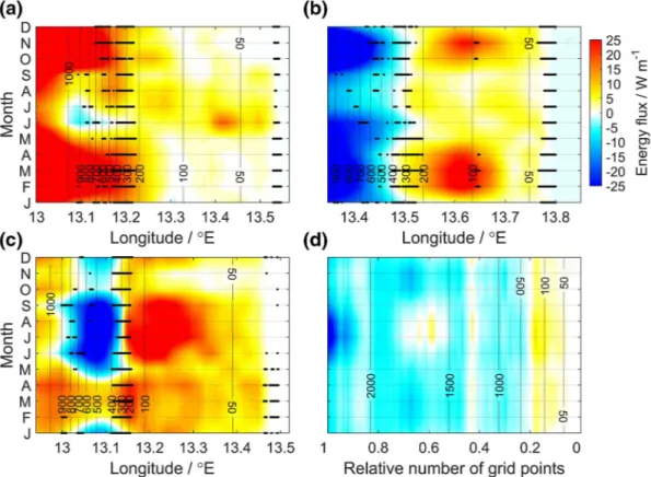
Figure 7. Seasonal vertically integrated onshore energy flux along section (a) C1, (b) C2, and (c) C3; black dots are supercritical points along the sections. Positive values indicate energy flux in onshore direction. (d) Seasonal spatially averaged vertically integrated onshore energy flux as a function of relative number of grid points. Black dashed lines with numbers are isobaths (unit: m).
Next, we calculate the onshore energy flux for the whole domain. For every grid point, we determine the shortest distance to the coast. The corresponding direction is regarded as the onshore direction. If there is the same shortest distance to different grid points at the coast, we use the average direction. Meanwhile, we classify each grid point in the whole domain according to its water depth and divide the number of grid points shallower than a certain depth by the total number of grid points (not including land grid points).
In this way, the relative number of grid points is 0 at the coast and 1 at the deepest grid point. The onshore energy flux as a function of months and the relative number of grid points is shown in Figure 7(d) (note that the right side corresponds to the coast). Although the flux shows strong seasonal variability for a certain cross-shore section, the spatially averaged flux over the whole domain changes only weakly throughout the year.
Therefore, we calculate the seasonal energy generation anomaly (value of each month minus the tempo- rally averaged value over the year), dissipation anomaly, and slope criticality as functions of the relative number of the grid points (Figures 8(a)–8(c)). The temporally averaged values of energy generation and dis- sipation are shown in Figure 8(d). Energy generation mostly occurs in water depths between 200 and 500 m for all months and its seasonal variability mainly appears in regions shallower than 1,000-m depth, which reflects that generation sites lie approximately along the 400-m isobaths. Both the maximum and minimum values appear in austral winter but total energy generation between 100 and 1,000 m does not vary signifi- cantly over the year. During austral winter, the depth range of enhanced values of generation (larger than 6 × 10⁴ W m–2) is narrower (around 300–500 m), which suggests that energy generation is more spatially confined. For the whole domain, the seasonal variations of energy generation is small compared to the temporally averaged values (cf., Figures 8(a) and 8(d)). Existing seasonal variations in the energy generation (Figure 8(a)) are due to the seasonally varying stratification associated with the initial temperature and sa- linity fields taken from observations that result in slightly varying supercritical/critical regions (Figure 8(c)).
Energy dissipation is more uniform over all depth ranges than energy generation. The highest temporally averaged value appears between 0 and 50 m (Figure 8(d)), a region that shows particularly weak seasonality (Figure 8(b)). A strong seasonal cycle of dissipation is found for areas with water depths between 50 and Figure 8. Seasonal anomaly of the spatially averaged energy (a) generation and (b) dissipation. (c) Seasonal spatially averaged slope criticality. (d) Temporally averaged energy generation and dissipation over the whole year. Dashed lines with numbers are isobaths (unit: m).
100 m as well as between 100 and 1,000 m. While in the shallower depth range maximum dissipation is found during February/March and October/November, for the deeper depth range maximum dissipation appears during June–August.
4. Discussion and Conclusions
Tidally generated internal waves play an important role in providing energy for turbulent mixing in the ocean (Munk & Wunsch, 1998). On the Angolan shelf, mixing processes related to ITs are thought to repre- sent a vital controlling factor for biological productivity (Ostrowski et al., 2009) and water mass properties (Tchipalanga et al., 2018). The results of case 0, a high-resolution simulation for July, are used to study the generation of IT, its onshore propagation, and its impact on mixing and water mass properties. The main generation sites of the ITs are along the continental slope between the 200- and 500-m isobaths. During aus- tral winter, the distance between two consecutive fronts is about 10 km along section C1 (Figure 4(a)). En- hanced baroclinic velocities along tidal beams suggests the appearance of ITs on the shelf and are the result of the interaction of the barotropic tide with critical/supercritical topography (Lamb, 2014). Beside the pri- mary M2 IT beam originating at the upper critical point of the main supercritical region at the continental slope, a secondary M2 tidal beam is identified along section C1 (Figure 4(a)) originating farther offshore. It modulates the vertical structure of the baroclinic current and likely contributes to the formation of the sec- ond-mode ITs. As the ITs propagate onshore, the cross-shore velocity shear increases (Figure 4(b)), which results in enhanced near-coastal mixing. Consistently, the temperature/density is decreased/increased in a near-surface layer and increased/decreased beneath it with the temperature/density anomalies increas- ing toward the coast. Note that if there were no tidal forcing, the waters at the surface would cool less in near-coastal regions than in regions far from the coast over time due to spatially uniform vertical mixing of the horizontally homogeneous initial temperature profile (Davidson et al., 1998). To verify that the model background diffusion can be indeed neglected against tidal mixing, we examine the temperature anomaly after a period of 20T on the westward extended section C1 (west to 11.5°E) of case 13, a model run without tidal forcing. Changes in temperature are less than 0.03°C in the whole domain with maxima in tempera- ture anomaly profiles being smaller near the coast (not shown). This implies that the background diffusion in our simulations is not a significant contributor to the stratification changes of cases 0–12. The stronger cooling of SST near the coast in our simulation is thus a consequence of the ITs.
As mentioned above, the high productivity during austral winter is not supported by upwelling due to up- welling-favoring winds, which are in their weakest phase during that period. Here, we have explored the possibility that seasonal stratification variations impact IT activity representing a mechanism that supports seasonal variability in near-coastal SSTAs and primary productivity. The total energy generation at the main generation site differs only slightly between July and March (Figure 8(a)), which suggests the seasonal vari- ability of energy generation is weak. The energy dissipation and onshore flux show seasonal variability with high spatial variability in the whole domain (Figures 5(e)–5(h)) but the spatially averaged onshore energy flux is only slightly enhanced in austral winter representing a period of weaker stratification (Figure 7(d)).
Hall et al. (2013), based on 2D continental slope/shelf simulations, found that stronger stratification on the shelf favors onshore energy flux, while for weaker stratification the energy flux is substantially reduced.
In their weak stratification case, the pycnocline is at the depth of the critical slope at around 600-m depth with very weak or no stratification on the shelf. However, on the Angolan shelf, the pycnocline is always shallower than 40 m and the main IT activity occurs shallower than 200 m. In fact, even the relatively weak stratification in austral winter is still strong enough to be favorable for M2 tidal energy transmission onto the Angolan shelf (Figure 2(d)). However, in terms of the energy budget, our results show only a weak seasonality in the spatially averaged energy generation at the continental slope, energy flux onto the shelf, and dissipation near the coast. Nevertheless, some IT characteristics show seasonal variability: the SSVD shows stronger signals along the shelf in July compared to March (Figures 5(a) and 5(b)) which is generally consistent with the observations of Ostrowski et al. (2009) that ITs/internal waves are more coherent and have larger amplitudes in austral winter compared to austral summer.
To address the identified seasonality in changes of hydrographic properties, we calculate the potential en- ergy (PE) change (i.e., the PE at the end of the model runs minus the initial PE) as an integral measure of mixing occurring during the model runs. For each water column, the PE is
PE d z t gzdz, ,
(9) where ρ(z,t) is the density, g the gravitational acceleration, and d is a predefined depth no more than the local water depth. The initial PE is computed from the initial fields for each case (see Section 2.2) that are derived from observations. Although the observed seasonal stratification used in the simulations is mod- ulated by tidal mixing, this effect should be small as the observed data used to derive the climatology are from hydrographic water-column profiles taken between the 200- and 800-m isobaths, while the strongest simulated tidal mixing occurs in regions shallower than 50-m water depth. The PE at the end of the model runs is a temporally averaged value over the last 2T of each case. Figure 9(a) shows the PE change over the whole water column and over the upper 20 m temporally averaged over all months (cases 1–12). The PE change over the whole water column is large in the area of the upper continental slope and shelf. It shows a narrow local maximum at about 400-m depth which corresponds to the region where the slope is critical/
supercritical for all months. When looking at PE change over the upper 20 m, it becomes evident that most of the PE change occurs away from the surface layer. It shows a maximum close to the coast in water depths shallower than 50 m, which is very much in accordance with the SSTA also temporally averaged over all months (cases 1–12) revealing enhanced values in water depths shallower than 50 m as well, with the max- imum anomaly at the coast (Figure 9(a)). The simulated mean difference between SSTA at the coast and further offshore is about 0.4°C defining a near-coastal cross-shore SST gradient that is established due to IT mixing (Figure 9(a)).
The seasonal cycle of the PE change over the whole water column on the shelf (0–200 m depth) is charac- terized by a maximum in July (main upwelling season during austral winter) with a secondary maximum in December/January (secondary upwelling season) (Figure 9(b)). Minima occur in March (main down- welling season) and November (secondary downwelling season). The maximum in austral winter is pre- sumably because the greater baroclinic velocity shear (Figures 6(c) and 6(d)) in combination with weaker stratification (Figures 6(e) and 6(f)) leads to lower Richardson numbers and enhanced mixing according to the applied KPP scheme. The PE change at the location of critical/supercritical slope at about 400-m depth (IT generation sites) is characterized instead by a weak seasonal cycle (Figure 9(b)), which is in agreement with a permanent criticality of the continental slope (Figure 8(c)) associated with the weaker seasonal cycle of the stratification at that depth (Figure 2(d)). As the spatially averaged energy generation shows weak seasonal variations, the amount of energy on the shelf available for mixing is similar throughout the year.
The seasonal cycle of the SSTA is in general agreement with the seasonal cycle of the PE change over the upper 20 m (Figure 9(c)). Strongest cooling in water depths shallower than 50 m is found in July (austral winter) in correspondence to the period of strongest PE change. Similarly strong cooling of the near-coast- al water is found during the secondary upwelling season in December/January, with weakest cooling in March and October/November, representing the main and secondary downwelling seasons, respectively.
The peak-to-trough amplitude of the seasonal cycle of the near-coastal SSTA is about 0.4°C. Further off- shore (50–400 m depth), there is a similar seasonal cycle in PE change and SSTA, but with smaller ampli- tude (about 0.2°C for SSTA).
Overall, the background stratification shows a substantial seasonal variability (Figure 2(d)), which results in a seasonality of some IT characteristics (Figure 6). However, the background stratification primarily represents the preconditioning for the mixing and is the reason, in our simulations, for the seasonal cycle of the spatially averaged PE change in the upper ocean on the shelf. The weaker stratification that eventually causes stronger mixing on the shelf and particularly near the coast results in larger near-coastal SSTAs and thus in enhanced cross-shore SST gradients in the main and secondary upwelling seasons compared to the main and secondary downwelling seasons characterized by stronger stratification.
It is concluded that with about the same amount of IT energy available on the shelf throughout the year, the water column can be much more effectively mixed during months with a weak stratification, for example, during July, compared to months with a strong stratification, for example, during March. The strongest
near-surface mixing thereby always occurs close to the coast in water depths shallower than 50 m resulting in larger negative SSTAs along the coast being most pronounced during austral winter.
Since the availability of satellite retrievals of winds, SST, and chlorophyll, it has become evident that in tropical upwelling regions equatorward of about the 20° circle of latitude, the seasonal variability of surface productivity and cross-shore SST gradients is often in opposition with the seasonal variability of alongshore wind stress (e.g., Thomas et al., 2001). For example, the tropical eastern boundary upwelling system off Peru (6°–18°S) shows a seasonal maximum of chlorophyll and cross-shore temperature gradient during austral summer, when the alongshore winds reach a seasonal minimum (Echevin et al., 2008). It is possible Figure 9. (a) Annual mean PE change over the whole water column (black solid line, left axis) and over the upper 20 m (black dashed line, left axis) and annual mean SST anomaly (blue solid line, right axis). Note that the black solid and dashed lines are identical for water depths shallower than 20 m. Vertical black dashed lines with numbers are isobaths (unit: m). (b) PE change over the whole water column as function of month of the year averaged in the area with water depths shallower than 200 m (solid line) and at the depth of maximum PE change over the whole water column at a water depth about 400 m (region of critical/supercritical slope). (c) PE change over the upper 20 m (black, left axis) and SST anomaly (blue, right axis) as function of month of the year averaged in the area 0–50 m water depth (solid lines) and 50–400 m water depth (dashed lines). PE, potential energy; SST, sea surface temperature.
that the interplay between ITs and the seasonal cycle of stratification also contributes to the seasonality of near-coastal cooling and upward nutrient flux in other tropical upwelling regions.
Our work provides a preliminary framework for understanding the 3D generation and propagation of ITs and their seasonal variations on the Angolan shelf. Yet there are still relevant processes that need to be ad- dressed in future work. For example, our limited model resolution does not allow for nonhydrostatic short internal solitary waves to develop. These nonlinear ISWs, which are suggested to vary seasonally along the Angolan shelf (Ostrowski et al., 2009), are missing in our simulations. They develop from the disintegration of ITs (Apel, 2003; Lamb, 2004) and may affect surface cooling and nutrient supply to the euphotic zone by the formation of wave-driven overturning circulations or by elevated velocity shear and wave breaking (Vlasenko & Hutter, 2002; S. Zhang et al., 2015). Resolving ISWs would likely not significantly impact the total energy dissipation on the shelf (Lamb, 2014), but it could affect the distribution of the dissipation both horizontally and vertically. However, ISW simulations would require a horizontal resolution of few meters, which cannot be achieved in the current 3D model framework, and 2D simulations are likely a better op- tion to address the potential role of ISWs in the upward nutrient supply on the Angolan shelf. On the other hand, observational estimates of mixing parameters in the Angolan upwelling region are urgently required to validate our model results. Measurements by microstructure shear sensors that can be used to estimate the dissipation rate of turbulent kinetic energy and turbulent eddy diffusivities are now possible for periods of up to 1 month using autonomous observatories (e.g., Merckelbach et al., 2019). From such data sets, the variability of mixing parameters and associated vertical turbulent heat and nutrient fluxes in the upwelling region could be determined (see Schafstall et al., 2010). Furthermore, these data sets could also yield further insight into the validity of our model approach, that is, the neglection of higher-resolution nonhydrostatic effects, and the appropriateness of the applied KPP mixing scheme.
Of course, the realism of our 3D simulations could be improved by the inclusion of wind, buoyancy forc- ing, a realistic boundary circulation, and CTWs, which would make it possible to study the variability of IT mixing during specific climatic events such as Benguela Niños and Niñas. Indeed, as the resolution of 3D circulation models improves, our results suggest that including tides explicitly (or improved parameteriza- tions of tidal mixing) in such models could lead to significant improvement in their overall performance.
Data Availability Statement
The SAR image was acquired by the ERS-1 satellite and is downloaded from https://earth.esa.int/web/
guest/missions/esa-operational-eo-missions/ers/instruments/sar/applications/tropical/-/asset_publish- er/tZ7pAG6SCnM8/content/upwelling-angola. The MODIS SST data are downloaded from https://po- daac-opendap.jpl.nasa.gov/opendap/allData/modis. The sea level anomaly from TOPEX/ERS merged data is downloaded from http://apdrc.soest.hawaii.edu/datadoc/aviso_topex_mon_clima.php. The meridional wind from CCMP data is downloaded from http://data.remss.com/ccmp/v02.0/. The MITgcm code and related input files in our work can be accessed at https://doi.org/10.5281/zenodo.4422439.
References
Alford, M. H., Peacock, T., MacKinnon, J. A., Nash, J. D., Buijsman, M. C., Centurioni, L. R., et al. (2015). The formation and fate of internal waves in the South China Sea. Nature, 521(7550), 65–69. https://doi.org/10.1038/nature14399
Apel, J. R. (2003). A new analytical model for internal solitons in the ocean. Journal of Physical Oceanography, 33(11), 2247–2269. https://
doi.org/10.1175/1520-0485(2003)033<2247:ANAMFI>2.0.CO;2
Bachelery, M. L., Illig, S., & Dadou, I. (2016). Interannual variability in the South-East Atlantic Ocean, focusing on the Benguela Upwelling System: Remote versus local forcing. Journal of Geophysical Research: Oceans, 121, 284–310. https://doi.org/10.1002/2015JC011168 Brandt, P., Rubino, A., Alpers, W., & Backhaus, J. O. (1997). Internal waves in the Strait of Messina studied by a numerical mod-
el and synthetic aperture radar images from the ERS 1/2 satellites. Journal of Physical Oceanography, 27(5), 648–663. https://doi.
org/10.1175/1520-0485(1997)027<0648:IWITSO>2.0.CO;2
Buijsman, M. C., Klymak, J. M., Legg, S., Alford, M. H., Farmer, D., MacKinnon, J. A., et al. (2014). Three-dimensional double-ridge inter- nal tide resonance in Luzon Strait. Journal of Physical Oceanography, 44(3), 850–869. https://doi.org/10.1175/JPO-D-13-024.1 Buijsman, M. C., Legg, S., & Klymak, J. (2012). Double-ridge internal tide interference and its effect on dissipation in Luzon Strait. Journal
of Physical Oceanography, 42(8), 1337–1356. https://doi.org/10.1175/JPO-D-11-0210.1
Cacchione, D., & Wunsch, C. (1974). Experimental study of internal waves over a slope. Journal of Fluid Mechanics, 66(2), 223–239.
https://doi.org/10.1017/S0022112074000164 Acknowledgments
This work is supported by the project
“Oceanic Instruments Standardiza- tion Sea Trials (OISST)” of National Key Research and Development Plan (2016YFC1401300), the Taishan Scholars Program, and the China Scholarship Council. The moored ADCP data (https://doi.pangaea.
de/10.1594/PANGAEA.870917) were acquired within the SACUS project (03G0837A) supported by the German Federal Ministry of Education and Research. Further funding was received from the BANINO project (03F0795A) by the German Federal Ministry of Education and Research, from the EU FP7/2007–2013 under grant agreement 603521 PREFACE project, and from the EU H2020 under grant agreement 817578 TRIATLAS project. Temperature and salinity data (https://doi.pangaea.
de/10.1594/PANGAEA.868683) were acquired within the monitoring component of the Nansen Program, in cooperation with the Instituto Nacional de Investigacao Pesqueira (INIP) in Angola and funded by the Norwegian Agency for Development Cooperation (Norad). We would like to thank two anonymous reviewers who provided helpful comments that significantly improved the manuscript. Open access funding enabled and organized by Projekt DEAL.