Development of local Coupled Cluster response methods for properties and analytic gradients of excited states in extended molecular systems

Cluster response methods for

properties and analytic gradients of excited states in extended molecular

systems

Dissertation

zur Erlangung des Doktorgrades der Naturwissenschaften (Dr. rer. nat.) der Fakult¨at

- Chemie und Pharmazie - der Universit¨at Regensburg

vorgelegt von

Katrin Lederm¨ uller

Freundorfer

aus Vilshofen an der Donau

im Jahr 2014

Die Arbeit wurde angeleitet von: Prof. Dr. Martin Sch¨utz

Chapter 2:

K. Lederm¨uller, D. Kats and M. Sch¨utz

”Local CC2 response method based on the Laplace transform:

Orbital-relaxed first-order properties for excited states”

The Journal of Chemical Physics

139, 084111 (2013), doi: 10.1063/1.4818586

Chapter 3:

K. Lederm¨uller and M. Sch¨utz

”Local CC2 response method based on the Laplace transform:

Analytic energy gradients for ground and excited states”

The Journal of Chemical Physics

submitted (2014)

An dieser Stelle m¨ochte ich mich bei all denen bedanken, die zur Entstehung dieser Arbeit beigetragen haben. Mein besonderer Dank gilt dabei:

• Herrn Prof. Dr. Martin Sch¨utz f¨ur die M¨oglichkeit dieses Thema zu bearbeiten sowie f¨ur die Betreuung und Unterst¨utzung in dieser Zeit.

• HerrnProf. Dr. Bernhard Dickf¨ur die freundliche ¨Ubernahme der Zweitbegutachtung.

• DerStudienstiftung des deutschen Volkes f¨ur die finanzielle F¨orderung.

• Dr. Daniel Katsf¨ur seine Hilfsbereitschaft.

• Stefan Loibl f¨ur die vielen hilfreichen Diskussionen.

• Thomas Merzf¨ur seine Hilfestellung bei Anwendungs- und sonstigen Fragen.

• Klaus Ziereisf¨ur seine schnelle und kompetente Hilfe bei Computerproblemen.

• Neben den bereits genannten aktuellen und ehemaligen Kollegen nat¨urlich auch Dr. Denis Usvyat, Dr. Keyarash Sadeghian, Dr. Dominik Schemmel, Dr. Marco Lorenz,Oliver Masur,Gero W¨alz,David David,Matthias HinreinerundAlexander Schinabeckf¨ur die sch¨one gemeinsame Zeit am Arbeitskreis.

• Eva S., Eva W., Michi, Oli, Susanne, Tanja und Tobi f¨ur die gemeinsame Zeit w¨ahrend des Studiums und auch danach, die ohne sie viel langweiliger und trost- loser gewesen w¨are.

• Nicht zuletzt auch allen, die mich außerhalb des universit¨aren Umfelds unterst¨utzt haben, allen voran meinem MannAchimsowie meinen Eltern Friedaund Helmut.

1 Introduction 3

1.1 Coupled Cluster model CC2 for the ground state . . . 4

1.1.1 The CC2 model . . . 4

1.1.2 Density fitting approximation . . . 6

1.1.3 Local approximations . . . 7

1.1.4 Dressed integrals . . . 9

1.2 CC2 for excited states . . . 10

1.2.1 Singlet excited states . . . 11

1.2.2 Triplet excited states . . . 11

1.2.3 The local CC2 response methods DF-LCC2 and LT-DF-LCC2 . . . 13

1.3 Coupled Cluster diagrams . . . 18

1.4 Structure of the thesis . . . 20

2 Orbital-relaxed first-order properties 21 2.1 Introduction . . . 21

2.2 The electronic ground state . . . 22

2.2.1 The Lagrangian . . . 22

2.2.2 Linear z-vector equations . . . 25

2.2.3 Calculation of the intermediateB⁰ . . . 27

2.2.4 Calculation of properties . . . 31

2.3 Singlet excited states . . . 32

2.3.1 The Lagrangian . . . 32

2.3.2 Linear z-vector equations . . . 33

2.3.3 Calculation of properties . . . 39

2.4 Triplet excited states . . . 39

2.4.1 The Lagrangian . . . 39

2.4.2 Linear z-vector equations . . . 39

2.4.3 Calculation of properties . . . 43

2.5 Orbital-relaxed densities . . . 44

2.6 Test calculations . . . 46

2.6.1 Approximate Lagrangians for LT-DF-LCC2 . . . 47

2.6.2 Pair approximations and domains . . . 48

2.6.3 Number of Laplace quadrature points . . . 52

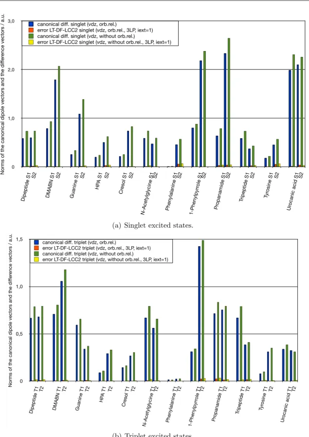
2.6.4 Accuracy of the local approximations . . . 54

2.6.5 Efficiency of the code . . . 61

2.7 Conclusions . . . 64

3 Analytic energy gradients 66 3.1 Introduction . . . 66

3.2 The electronic ground state . . . 68

3.2.1 The Lagrangian . . . 68

3.2.2 Derivation of the gradient . . . 69

3.3 Singlet excited states . . . 75

3.3.1 The Lagrangian . . . 75

3.3.2 Derivation of the gradient . . . 76

3.4 Triplet excited states . . . 79

3.4.1 The Lagrangian . . . 79

3.4.2 Derivation of the gradient . . . 79

3.5 Hybrid method (LT-)DF-LCC2 . . . 81

3.6 Test calculations . . . 82

3.6.1 Accuracy of the local methods . . . 82

3.6.2 Efficiency of the code . . . 89

3.7 Conclusions . . . 95

4 Summary 97

Bibliography 100

A Coupled Cluster diagrams 105

B Symmetry of the external-external part of B⁰ 109

Introduction

The excitation of electrons in molecules plays an important role for many applications in chemistry and physics. Thus, there is a need for theoretical methods based on quantum mechanics, which are able to describe such processes and complement the experimental techniques.

The behaviour of molecules in the ground state and in electronically excited states can be analysed based on the related potential energy hypersurfaces (PES).^{1, 2} The PES describes the energy of an eigenstate of the electronic Schr¨odinger equation as a function of the nuclear positions. The separation of the system into an electronic part and a nuclear part, which contributes as a parameter to the electronic part, is enabled by the Born-Oppenheimer approximation, which is one of the basic concepts in quantum chemistry.³ This partitioning into an electronic and a nuclear part is justified by the much faster movement of the electrons compared to the movement of the nuclei. Hence, the electronic structure of a molecule can be considered at a fixed nuclear geometry and only the electronic Schr¨odinger equation has to be solved. After a change of the electronic structure caused by an excitation the nuclei subsequently relax due to the new potential in order to reach a stable state.

For the description of photophysical processes the PES of the ground and the excited states have to be analysed. Molecular properties calculated at particular geometries can complete the picture. Stationary points of the PES are equilibrium and transition structures of molecules, and thus of great interest in chemistry and physics as has been discussed in many publications about this topic, e.g. in the context of photochemistry and the special topic of photocatalysis.^{4, 5} For locating stationary points on the PES the gradient of the energy with respect to nuclear displacements has to be calculated.

Therefore, a variety of quantum chemical methods has been developed, which are able

to describe the electronic structure of molecules and to predict molecular properties.

One example for a post-Hartree-Fock method, i.e. a method describing the correlation of the electrons based on an underlying Hartree-Fock (HF) calculation, is the Coupled Cluster (CC) method.^6–8 Excitation energies and properties of the ground and the excited states can be obtained via CC response theory.⁹ A general problem of correlation methods like CC, limiting their applicability to larger molecules, is the steep scaling of the computational cost with the size of the molecules.

The aim of this thesis is the development of orbital-relaxed properties and gradients with respect to nuclear displacements within the Coupled Cluster model CC2, which are also applicable to extended molecular systems. The following sections give a short introduction to the CC2 method for the ground state (section 1.1) and electronically excited states (section 1.2). Moreover, two concepts are presented, which were used in the context of this thesis in order to reduce the computational cost, namely density fitting and local correlation methods. In section 1.3 the diagrammatic techniques are explained, which help to obtain practical equations from the common CC expressions.

Finally, section 1.4 gives an outline of the thesis.

1.1 Coupled Cluster model CC2 for the ground state

1.1.1 The CC2 model

Coupled Cluster is a post-Hartree-Fock method describing the correlation of the elec- trons.^6–8 The general CC wavefunction can be written as

|CCi= exp(T)|0i (1.1)

with the Hartree-Fock reference determinant |0i and the cluster operator T, which is defined as

T=X

i

Ti , with Ti =X

µi

tµiτµi . (1.2)

τµi are excitation operators and tµi the corresponding amplitudes. For singlet substitu- tions, as they occur for the electronic ground state and for singlet excited states, the

single and double excitation operators needed for the CC2 model are defined as τ_i^a = a^†_aαaiα+a^†_aβaiβ ,

τ_ij^ab = 1

2(a^†_aαaiα+a^†_aβaiβ)(a^†_bαajα+a^†_bβajβ), (1.3) in terms of the elementary second quantization creation and annihilation operators a^† anda(the indexiαimplies a spin orbital related to a spatial orbitalitimes spin function α,etc.). The double excitation operators are symmetric with respect to the permutation of the electrons, i.e. τ_ij^ab =τ_ji^ba.

The CC ground state correlation energy is calculated as

E₀^CC =h0|exp(−T)Hexp(T)|0i=h0|H|CCi, (1.4) where H is the normal ordered Hamiltonian consisting of the Fock matrix F and the fluctuation potential V,

H=F+V . (1.5)

By employing the Baker-Campbell-Hausdorff-expansion, exp(−T)Hexp(T) = H+ [H,T] + 1

2![[H,T],T] + 1

3![[[H,T],T],T] +... , (1.6) the CC equations can be written using more convenient commutator expressions.

The computationally cheapest CC model, which is also used for excited state calcula- tions and includes dynamical correlation effects, is the CC2 model. It was proposed by Christiansenet al.¹⁰ as an approximation to the well-known CCSD (CC including single and double excitations) model. The summation in the CC2 cluster operatorTruns over single and double excitations (T = T1 +T2), thus the CC2 correlation energy can be written as

E₀^CC2 = h0|exp(−T1) exp(−T2)Hexp(T1) exp(T2)|0i

= D

0|Hˆ + [ ˆH,T2]|0E

. (1.7)

The correlation energy is explicitly labeled with the superscript CC2 to avoid confusion with the full energy including the HF contribution, which will occur in chapter 3. Oper- ators decorated with a hat represent operators similarity transformed by the exponent

of the singles cluster operatorT1, e.g.

Hˆ = exp(−T1)Hexp(T1) . (1.8)

A consequence of the similarity transformed operators is the occurrence ofdressed inte- grals, which will be discussed in section 1.1.4. The CC2 amplitudes are determined by the equations

Ωµ1 = D

˜ µ1

Hˆ +h

H,ˆ T2

i 0E

= 0 , Ωµ2 = D

˜ µ2

Hˆ + [F,T2] 0E

= 0 . (1.9)

h˜µ1| and hµ˜2| are contravariant configuration state functions (CSFs) projecting onto the singles and doubles manifold.¹¹ The covariant ket and contravariant bra CSFs for singlet states are defined as

|Φ^a_ii=τ_i^a|0i , |Φ^ab_iji=τ_ij^ab|0i , hΦ˜^a_i|= 1

2hΦ^a_i|, hΦ˜^ab_ij|= 1

6 2hΦ^ab_ij|+hΦ^ab_ji|

. (1.10)

The amplitudes related to double substitutions are correct only to first order with respect to a Møller-Plesset (MP) partitioning of the Hamiltonian, whereas the full exp (T1) part of the CC ansatz is retained to provide partial orbital relaxation.

1.1.2 Density fitting approximation

Compared to computationally cheap methods, like density functional theory (DFT), canonical CC2, although being one of the cheapest CC models, is computationally rather expensive and the scaling behaviour of the computational cost with molecular size N is O(N⁵). Therefore, for extended molecular systems DFT might be the sole applicable method for the calculation of excited states, although it is unreliable and often fails qualitatively, if charge transfer (CT) states, Rydberg states or excitations of extendedπ systems are involved.^12–14 In order to reduce the computational cost of CC2 for ground and excited state calculations the density fitting approximation (DF)^15–17 is applied to the four-index two-electron integrals,

(mn|pq) = Z

Φ^∗_m(r₁)Φ^∗_p(r₂)r₁₂⁻¹Φn(r₁)Φq(r₂)dr₁dr₂ . (1.11)

Within this approximation the four-index integrals are decomposed into three-index objects, i.e.

(mn|pq)≈X

P

(mn|P)c^P_pq , with c^P_pq =X

Q

J⁻¹

P Q(Q|pq) . (1.12) The fitting coefficients c^P_pq are determined by the minimization of an error functional.

The capital letters P, Q index the auxiliary fitting functions and JP Q = (P|Q) is an element of their Coulomb matrix. The indices m, n, p, . . . denote general molecular orbitals.

There are highly efficient CC2 and scaled opposite-spin (SOS) CC2 implementations using this approach for properties and analytic gradients of the ground state and excited states.^18–23 However, DF reduces only the prefactor, but not the scaling with molecular size N: canonical DF-CC2 still scales as O(N⁵).

1.1.3 Local approximations

For a further reduction of the computational cost the application of local approximations to DF-CC2 has been proposed.^24–29 The basic idea of local methods is to utilize the short-range nature of the dynamic electron correlation in nonmetallic systems, but this is only possible in a basis of spatially localized orbitals. The canonical orbitals resulting from a Hartree-Fock calculation are completely delocalized and thus inappropriate for local methods. A spatially localized basis can e.g. consist of localized molecular orbitals (LMOs) to span the occupied space, and projected atomic orbitals (PAOs) for the virtual space.^{30, 31} The molecular orbitals (MO) are in general expanded in a non-orthogonal atomic orbital (AO) basis χµ with the metric S_µν^AO=hχµ|χνi,

φp =X

µ

χµCµp. (1.13)

AOs are labeled by greek letters. The LMO coefficient matrix L is obtained from the canonical occupied coefficients via unitary transformation,

Lµi =X

¯i

C_µ^o¯iW¯ii , (1.14)

with the occupied part of the canonical coefficient matrix C^o. For canonical occupied orbitals the indices ¯i,¯j, . . . are used, for LMOs the indices i, j, . . . Different choices for

the unitary matrixWare possible, in the following it is assumed, that the Pipek-Mezey procedure is used, which minimizes the number of atoms on which the LMO is located.³² Another well-known localization scheme is the Boys procedure, which maximizes the distance between the orbital centroids.³³ The PAOs, which span the virtual space, are obtained via projection of the atomic orbitals onto the virtual space³⁰with the projector matrix P,

Pµr =X

aνρ

C_µa^v C_aν^v†S_νρ^AOδρr =X

a

C_µa^v Qar . (1.15)

C^v is the virtual part of the canonical coefficient matrix andQthe matrix, which trans- forms from canonical to PAO basis. For canonical virtual orbitals the indicesa, b, . . . are used, for PAOs the indicesr, s, . . . The LMOs are mutually orthogonal, while the PAOs are orthogonal to the LMOs, but not mutually. The metric S of the PAOs is obtained as

S=P^†S^AOP=Q^†Q . (1.16)

In the spatially localized LMO/PAO basis local approximations can be introduced. In local CC2 methods the singles quantities remain unrestricted, whereas the doubles are restricted to excitations from LMOs ij on a truncated pair list to PAOs in the cor- responding pair domain [ij].^{24, 26} For the electronic ground state the restrictions are obtained straightforwardly from distance criteria. The LMO pair list for the electronic ground state contains all pairs of LMOs up to a particular LMO interorbital distance Rg. The domains truncating the pair-specific virtual space are obtained by unifying the corresponding orbital domains, which are built by applying the Boughton Pulay procedure.³⁴ The BP orbital domain [i] comprises the PAOs arising from AOs, which considerably contribute to the particular LMO i. The LMO interorbital distances for the construction of the pair list are measured as the closest distance between the two sets of nuclei related to the relevant BP domains.

1.1.4 Dressed integrals

Dressed integrals occur due to the operators, which are similarity transformed by the exponent of the singles cluster operator T1, c.f. eq. (1.8). They are calculated as

(mnˆ|pq) = X

µνρσ

(µν|ρσ)Λ^p_µmΛ^h_νnΛ^p_ρpΛ^h_σq , (1.17)

with the coefficient matrices Λ^p and Λ^h in LMO/PAO basis, which contain the singles ground state amplitudestµ1,

Λ^p_µr =Pµr −X

ir^′

Lµitⁱ_r′Sr^′r , Λ^p_µi =Lµi , Λ^h_µr =Pµr , Λ^h_µi =Lµi+X

r

Pµrtⁱ_r . (1.18) As discussed in section IIA of Ref. 29, for the Fock matrix internal and external dressing are distinguished. The Fock matrix contains the one-electron integralshµν and the two- electron integrals (µν|ρσ). Internal dressing refers to the use of the coefficient matrices Λ^p and Λ^h in the contraction with the two-electron integrals inside the Fock matrix,

fˆµν =hµν + 2X

kρσ

Λ^p_ρkΛ^h_σk[(µν|ρσ)−0.5(µρ|σν)]. (1.19)

Internal dressing actually involves contractions with the fluctuation potential (evident, when the similarity transformation with exp(T1) is carried out after the Hamiltonian is written in normal ordered form) and is therefore of first-order. External dressing, on the other hand, means using these coefficient matrices for the transformation of the (internally dressed) Fock matrix ˆfµν to the MO basis,

fˆpq =X

µν

fˆµνΛ^p_µpΛ^h_νq , (1.20)

and is of zeroth-order.

Dressed integrals and other objects containing such integrals are labeled by a hat. If not explicitly stated otherwise, ˆfpq implies internal and external dressing.

1.2 CC2 for excited states

Time-dependent (TD) response theory is a widely-used and general framework providing access to excitation energies and other properties of excited states for various wavefunc- tion approaches. It starts from the time-dependent Schr¨odinger equation, which contains a time dependent-perturbation. The use of TD response theory is well established e.g.

in the context of Hartree-Fock (TD-HF),³⁵ density functional (TD-DFT),^{12, 36} or Cou- pled Cluster theory (TD-CC).^{9, 37–39} Also TD response methods for non-conventional, variational Coupled Cluster ans¨atze have been discussed.^{40, 41} A detailed description of the traditional, non-variational Coupled Cluster linear response theory can be found in reference 9.

First, an appropriate time-averaged quasienergy Lagrangian has to be specified,^42–44 from which then the linear response function is obtained by differentiation (rather than from the time-averaged quasienergy itself, as for variational methods). The excitation energies are obtained as a property of the electronic ground state, namely as the poles of the linear response function, i.e. the frequency-dependent polarizability (FDP). Applied to CC, the result is, that the excitation energies are obtained as the eigenvalues of the JacobianA,

Aµiνj = ∂Ωµi

∂tνj

. (1.21)

The CC response function differs from the exact one, but the additional terms do not affect the location of the poles. Thus CC theory reproduces the exact pole structure, from which the excitation energies of the system are obtained. The equation-of-motion Coupled Cluster (EOM-CC) method,^45–49 approaches excited states from the CI per- spective, but has close relationships to TD-CC response. The excitation energies and densities of TD-CC response and EOM-CC are equivalent.

There is a hierarchy of CC models employed in the context of TD-CC response theory, differing in the level of truncation of the cluster operator, and in simplifications made in the CC amplitude equations based on many-body perturbation theory.⁵⁰ The CC2 model, which is in the focus of this thesis, is the computationally cheapest model of this hierarchy, which does not neglect dynamical correlation effects.¹⁰ The CC2 model produces rather accurate results for excited states, provided that they are dominated by singles substitutions.

Canonical^18–21 as well as local^24–28 CC2 response methods were presented for the calcu-

lation of excitation energies and orbital-unrelaxed first-order properties. Canonical and local implementations both use the densitiy fitting approximation (cf. section 1.1.2) to decompose the four-index integrals into three-index quantities. The methods were developed for singlet and triplet excited states, which both play an important role in spectroscopy.

1.2.1 Singlet excited states

The CC2 Jacobian for singlet excited states takes the form

Aµiνj = hµ˜1|[ ˆH, τν1] + [[ ˆH, τν1],T2])|0i hµ˜1|[ ˆH, τν2]|0i h˜µ2|[ ˆH, τν1]|0i h˜µ2|[F, τν2]|0i

!

. (1.22)

τµi are the singlet excitation operators defined in eq. (1.3), and h˜µi| the contravariant CSFs for singlet states defined in eq. (1.10). For excitation energies it is sufficient to solve the right eigenvalue problem,

AR^f =ωfMR^f , (1.23)

to obtain the right eigenvectorR^f and excitation energyωf for statef. M is the metric of contra- and covariant CSFs. The Jacobian is not symmetric, thus for the calculation of properties also the left eigenvalue problem,

L˜^fA=ωfL˜^fM , (1.24)

has to be solved to obtain the contravariant left eigenvector ˜L^f. Details about solving these equation systems and the corresponding working equations can be found in Ref.

24 and 25 for the DF-LCC2 method and in Ref. 26 and 27 for the LT-DF-LCC2 method.

The differences between these two local CC2 methods will be discussed in section 1.2.3.

Details about the calculation of properties will be discussed in chapter 2.

1.2.2 Triplet excited states

Triplet excited states were introduced into the canonical DF-CC2 response method in Ref. 20, and later also implemented in the framework of the local LT-DF-LCC2 method.²⁸ For triplet substitutions the excitation operatorsτ for single and double excitations are

defined as

τ_i^a = a^†_aαaiα−a^†_aβaiβ ,

τ_ij^ab = (a^†_aαaiα−a^†_aβaiβ)(a^†_bαajα+a^†_bβajβ). (1.25) Contrary to the singlet case, the triplet double substitution operators have no permuta- tional symmetry (τ_ij^ab 6=τ_ji^ba), but they are linearly dependent according to

τ_ij^ab+τ_ji^ba+τ_ji^ab+τ_ij^ba = 0. (1.26) To get rid of these redundancies symmetrized operators of the form

(+)

τ_ij^ab =τ_ij^ab+τ_ji^ba, ∀ a > b, i > j ,

(−)

τ_ij^ab =τ_ij^ab−τ_ji^ba, ∀ (ai)>(bj) , (1.27) are introduced, which fulfill the symmetry relations

(+)

τ_ij^ab =

(+)

τ_ji^ba =−

(+)

τ_ij^ba =−

(+)

τ_ji^ab and

(−)

τ_ij^ab =−

(−)

τ_ji^ba. (1.28)

The covariantket and contravariantbra CSFs for triplet states are defined as

|Φ^a_ii=τ_i^a|0i , |

(+)

Φ^ab_iji=

(+)

τ_ij^ab|0i , |

(−)

Φ^ab_iji=

(−)

τ_ij^ab|0i , hΦ˜^a_i|= 1

2hΦ^a_i| , h

(+)

Φ˜^ab_ij|= 1 8h

(+)

Φ^ab_ij| , h

(−)

Φ˜^ab_ij|= 1 8h

(−)

Φ^ab_ij| , (1.29) and the triplet singles and doubles cluster operatorsU1 and U2 as

U1 =X

ia

uⁱ_aτ_i^a, and U2 = X

a>b,i>j (+)

U_ab^ij

(+)

τ_ij^ab+ X

(ai)>(bj) (−)

U_ab^ij

(−)

τ_ij^ab . (1.30)

Thus the Jacobian A, for which the right (and for properties also the left) eigenvalue equation system has to be solved, takes for triplet excited states the form

Aµiνj =











h˜µ1|[ ˆH, τν1] + [[ ˆH, τν1],T2]|0i h˜µ1|[ ˆH,⁽⁺⁾τν2]|0i hµ˜1|[ ˆH,τ⁽⁻⁾ν2]|0i h⁽⁺⁾µ˜2|[ ˆH, τν1]|0i h⁽⁺⁾µ˜2|[F,τ⁽⁺⁾ν2]|0i 0 h⁽⁻⁾µ˜2|[ ˆH, τν1]|0i 0 h⁽⁻⁾µ˜2|[F,⁽⁻⁾τν2]|0i











. (1.31)

The cluster operatorTrefers to the ground state and therefore contains singlet excitation operators. The working equations for the left and right matrix-vector products in the context of the LT-DF-LCC2 method can be found in Ref. 28.

1.2.3 The local CC2 response methods DF-LCC2 and LT-DF-LCC2

The a priori specification of local approximations is rather straightforward for ground state amplitudes, but more intricate for eigenvectors of excited states, which can have Rydberg or CT character.24, 26, 51, 52 Two local CC2 response methods were developed (both including density fitting), which are discussed in the following. Within both methods the local basis is spanned by LMOs and PAOs and restricted pair lists and domains are introduced only for the doubles quantities, the singles remain unrestricted.

The latter is important due to the neglect of explicit orbital relaxation in the (time- averaged) Lagrangian, which otherwise would cause fictitious additional poles originating from the underlying time-dependent Hartree Fock solution.⁹ Explicit orbital relaxation is added afterwards for the calulation of orbital-relaxed properties and energy gradients as will be demonstrated in the chapters 2 and 3.

DF-LCC2

The DF-LCC2 method was developed for excitation energies²⁴ and first-order proper- ties.²⁵ As discussed in detail in section IIB of Ref. 24, it determines the local approxima- tions by an a priori analysis of the untruncated CIS (configuration interaction singles) wavefunction of the state of interest, which can be calculated quite simply and fast.

The first step towards the excited state pair list is to determine a list of important LMOs.

For every LMO a weight is calculated based on the CIS coefficients and the LMOs are added to the list of important LMOs in order of their weights, starting with the highest one, until the sum of their corresponding weights reaches a thresholdκe. The remaining

LMOs with low weights are neglected. The CIS wavefunction is normalized, thus setting κe= 1 leads to a full list of important LMOs. The final excited state pair list comprises all pairs of LMOs on this list of important orbitals, all other pairs of LMOs up to a certain interorbital distance Rex, and the pairs of the ground state pair list.

The excited state pair domains [ij], which restrict the virtual space for double excitations from the corresponding pair of LMOs ij, are obtained by unifying the excited state orbital domains [i] and [j]. For an important LMO ithe excited state orbital domain [i]

is the union of the corresponding ground state orbital domain and an additional domain.

This additional domain is obtained by applying the Boughton Pulay procedure³⁴ to orbitals, which are constructed using the CIS coefficients. For unimportant orbitals the excited state orbital domain is equal to the ground state domain.

Within the DF-LCC2 method the singles and doubles eigenvalue equations have to be solved explicitely, it is not possible to construct an effective singles eigenvalue problem as can be done in canonical CC2 (cf. next paragraph). Moreover, the a priori ap- proximations obtained from the CIS wavefunction cause problems, if the simpler theory provides qualitatively wrong wavefunctions for the excited states. Hence, another local CC2 method called LT-DF-LCC2 was developed, which employs the Laplace transfor- mation. In this method the eigenvalue equations are reduced to an effective singles eigenvalue problem like in canonical CC2 and multistate calculations with state-specific local approximations are enabled.^26–28

LT-DF-LCC2

In the following the Einstein convention is employed for conciseness, i.e. repeated indices are implicitly summed up. Summations are only written explicitly, if it is necessary for clarity.

The concept of partitioning the eigenvalue equations using Laplace transformation is applied to the right and left eigenvalue equations and to the equations determining the Lagrange multipliers λ˜⁰ and ˜λ^f, which will be introduced in chapter 2. The formalism was derived for MP2,⁵³and adopted for local MP2⁵⁴and CC2²⁶methods. In the following the approach is explained using the example of the right eigenvalue equation system for singlet excited states. The right eigenvalue problem for the singlet Jacobian leads to a set of equations for the singles part of the eigenvector Rµ1, and a set of equations for

the doubles partRµ2,

Aµ1ν1Rν1 +Aµ1ν2Rν2 =ωRν1Mν1µ1 ,

Aµ2ν1Rν1 +Aµ2ν2Rν2 =ωRν2Mν2µ2 . (1.32) In canonical basis the doubles-doubles part of the Jacobian is diagonal,

Aµ2ν2 = ∆ǫµ2δµ2ν2 , with ∆ǫ¯^abi¯j =ǫa+ǫb−ǫ¯i−ǫ¯j . (1.33) ǫp is the energy of the canonical orbital p and δµ2ν2 is 1 for µ₂ = ν₂ and 0 otherwise.

Hence, an effective singles eigenvalue problem can be formulated and the doubles can be calculated on-the-fly,

Rµ2 = Aµ2ν1Rν1

ω−∆ǫµ2

, A^eff_µ1ν1(ω)Rν1 = Aµ1ν1Rν1 +Aµ1ξ2

Aξ2ν1Rν1

ω−∆ǫξ2

=ωMµ1ν1Rν1 . (1.34) The Laplace transform (LT) identity,

1 x =

Z∞

0

exp(−xt)dt ≈

nq

X

q=1

wqexp(−tqx) , (1.35)

can be employed to evaluate the denominator of the doubles expression and to calculate the doubles part on-the-fly,^{26, 53}

A^eff_µ1ν1(ω)Rν1 ≈Aµ1ν1Rν1 −Aµ1ξ2

nq

X

q=1

wqe^{−∆ǫξ2tq}e^ωtqAξ2ν1Rν1 . (1.36) This partitioning allows the formulation of the eigenvalue equation with local orbitals i, j, r, sfor the doubles, i.e.

A^eff_µ1ν1(ω)Rν1 = Aµ1ν1Rν1

−Aµ1irjs nq

X

q=1

sgn(wq)e^ωtqY_rt^v(q)Y_su^v(q)(Aktluν1Rν1)X_ki^o(q)X_lj^o(q)

= ωMµ1ν1Rν1 . (1.37)

Thus, the Laplace transform identity can be utilized to decompose the eigenvalue prob-

lem into an effective singles eigenvalue problem without losing the sparsity of the matrices in the local basis. The doubles can be calculated directly in the local basis as

R^ij_rs = −V_rt^ijV_su^ij(1 +PijPtu)

nq

X

q=1

sgn(wq)e^ωtq

×X_tv^v′(q)V_v^†′vX_uw^v ′(q)V_w^†′w( ˆB_vk^Pcˆ^P_wl)X_ki^o(q)X_lj^o(q) , (1.38) with the permutation operatorPpq, which permutes the orbital indices pand q, and an intermediate quantity ˆB_ai^P, which depends on the singles vector Rν1 (working equations can be found in Ref. 26, section IIB). Thus, in this local CC2 response method based on Laplace transform, denoted as LT-DF-LCC2, just an effective eigenvalue problem in the space of the untruncated singles determinants has to be solved (as in the canonical case) and the doubles part does not enter the Davidson diagonalization explicitly.

The quadrature point dependent matrices X_ij^o(q), X_rs^v(q) and Y_rs^v(q) appearing in eqs.

(1.37) and (1.38) were defined in Ref. 54 as

X_ij^o(q) = W_i^†_¯ie^{(ǫ¯i−ǫF)tq+14ln|wq|}W¯ij, X_rs^v(q) = Q^†_rae^{(−ǫa+ǫF)tq+14ln|wq|}Qas,

Y_rs^v(q) = VrtX_tu^v(q)V_us^†. (1.39) with the matrices W, transforming from occupied canonical orbitals to LMOs, and Q, transforming from virtual canonical orbitals to PAOs, which were already introduced in section 1.1.3. V^ij is the pseudoinverse of the corresponding PAO metric S^ij_PAO. ǫF

contains the energy difference between the highest occupied molecular orbital (HOMO) and the lowest unoccupied molecular orbital (LUMO),

ǫF = ǫHOM O−ǫLU M O

2 , (1.40)

and cancels in equation (1.37), but ensures that the exponential factor is for positivetq

always smaller than 1.

The quadrature points tq and the corresponding weights wq are obtained by a Simplex optimization procedure.^{26, 54} It has been shown, that only a small numbernq of Laplace quadrature points is needed to reach sufficient accuracy.26, 28, 29, 54

The LT approach can analogously be applied to triplet excited states,²⁸with the effective

singles eigenvalue problem

A^eff_µ1ν1(ω)Rν1 =Aµ1ν1Rν1 +(

(+)

Aµ1ξ2

(+)

Aξ2ν1 +

(−)

Aµ1ξ2

(−)

Aξ2ν1)Rν1

ω−∆ǫξ2

=ωMµ1ν1Rν1 . (1.41) The doubles can be calculated directly in the local basis as

(+)

R^ij_rs = −V_rt^ijV_su^ij(1− Pij)(1− Ptu) 2

nq

X

q=1

sgn(wq)e^ωtq

×X_tv^v′(q)V_v^†′vX_uw^v ′(q)V_w^†′w( ˆB_vk^Pˆc^P_wl)X_ki^o(q)X_lj^o(q) ,

(−)

R^ij_rs = −V_rt^ijV_su^ij(1− PijPtu) 2

nq

X

q=1

sgn(wq)e^ωtq

×X_tv^v′(q)V_v^†′vX_uw^v ′(q)V_w^†′w( ˆB_vk^Pˆc^P_wl)X_ki^o(q)X_lj^o(q) , (1.42) with the quantity ˆB_ai^P depending on the singles vectorRν1 (details and working equations can be found in Ref. 28, section IIA).

In LT-DF-LCC2 calculations adaptive, state-specific local approximations are employed for excited state doubles quantities, as explained in detail in section IIC of Ref. 26. As in the DF-LCC2 method the excited state pair lists usually contain all pairs of LMOs on the list of important orbitals, all other pairs of LMOs up to a certain interorbital dis- tanceRex, and all pairs of the ground state list. The size of the list of important LMOs is, as for DF-LCC2, regulated via a threshold κe, but the criterion is not constructed using the CIS coefficients. It is obtained by a L¨owdin like analysis of the untruncated diagonal pair doubles part U_rsⁱⁱ of the actual approximation Uµ2 to the eigenvector for each individual state.

The excited state domains are obtained in an adaptive procedure, also based on analysis of the actual approximation to the eigenvector. The orbital domains are determined by specifying an ordered list of important centers for each important LMO. The ground state domains then are augmented with further centers from this list until a threshold is reached by the least-squares optimization procedure introduced in section IIC of Ref. 26.

For unimportant orbitals the excited state orbital domain is equal to the ground state domain. The excited state pair domains are obtained by unifying the corresponding excited state orbital domains.

Contrary to the DF-LCC2 method, the local approximations are state-specific and re-

specified in every Davidson-refresh, thus they allow the eigenvectors to change their character during the Davidson process. If two states come energetically close, the lo- cal approximations of these states are unified. Thus, the LT-DF-LCC2 method is a multistate method in the same sense as canonical CC2.

1.3 Coupled Cluster diagrams

Starting from the common CC expressions based on the normal ordered second quan- tized operators and the particle-hole-formalism practical equations can be developed by employing diagrammatic techniques.⁵⁵ In the context of this thesis CC diagrams were used to obtain the starting equations for the Lagrangians, from which properties and the gradient with respect to nuclear displacements are obtained by differentiation as explained in detail in the chapters 2 and 3. The following outline is a revised version of section 2.4 in Ref. 56.

Operators are depicted as vertical interaction lines, which are connected by horizontal lines, that start or end at the vertex of an operator. Every vertex has an incoming and an outgoing horizontal line, symbolizing the action of the operator on an electron. The one-electron operators, i.e. the Fock and single excitation operators, have one vertex, the two-electron operators, i.e. the fluctuation and the double excitation operators, have two vertices. In literature, the diagrams are often rotated by 90^◦ compared to the diagrams in this thesis, which were obtained from the programccgen.⁵⁷

Starting from the Baker-Campbell-Hausdorff-expansion (eq. (1.6)) of the normal ordered second quantized Hamiltonian it can be demonstrated, that in CC theory only those diagrams contribute, in which all operators are connected by horizontal lines. There are some rules for the evaluation of such diagrams:

1. Horizontal lines pointing from the left to the right are hole lines representing oc- cupied orbitals denoted with the indicesi, j, k and so on. Horizontal lines pointing to the left are particle lines representing virtual orbitals denoted with the indices r, s, t and so on. Lines, which start or end at a bare excitation operator τµi, are dashed.

2. Every vertical line contributes an integral or an amplitude to the final expression, except for the lines, which represent a bare excitation operatorτµi. An element of the Fock matrix would be hout|F|ini, where out stands for the outgoing line and

(a) Diagrams contributing to hΦⁱ_r|[V, T¹]|0i.

(b) One of the diagrams contributing tohΦⁱ_r|[F, T¹]|0i.

Figure 1.1: Examples of CC diagrams.

in for the incoming one. The two-electron integrals are constructed following the scheme (out1 in1 |out2 in2), where the indices 1 and 2 denote the vertex.

3. The summation runs over all internal lines, i.e. the lines which are not connected to a bare excitation operator τµi.

4. The sign of a diagram is (−1)^h+l, where h is the number of hole lines and l the number of loops.

5. Every loop contributes a factor of 2. But if a loop directly links a singlet and a triplet vertex (without an operator in between), the factor is 0 and the dia- gram does not contribute. The vertices of the Hamiltonian are singlet vertices.

The triplet double excitation operators have one triplet and one singlet vertex, cf. eq. (1.25).

6. The projected atomic orbitals (PAOs), which are used in this work for spanning the virtual space in the local basis, are not mutually orthogonal. Thus each particle line, which directly links theket(on the right) with the bra(on the left) without an operator in between, contributes an element of the PAO overlap matrixS.

The procedure is in the following demonstrated for the examplary term hΦⁱ_a|[V, T1]|0i.

There are two diagrams corresponding to this term, which are shown in figure 1.1(a).

According to the first rule the hole lines are denoted as i and k, and the particle lines as r and s. The operators V and T1 contribute an integral and an amplitude to the expression (rule 2). The bra side does not contribute an amplitude, because only the bare excitation operatorτ_rⁱ is involved. The summation runs over all internal lines, that means all lines except the ones coming fromτ_rⁱ (rule 3). For the chosen example the two sums

X(ki|rs)t^k_s and X

(ri|ks)t^k_s (1.43)

are obtained. Applying the rules 4 to 6 yields the final expressions for the term hΦⁱ_a|[V, T₁]|0i, depending on the spin symmetry of hΦⁱ_r|. If hΦⁱ_r| is a singlet CSF, the result is

−2X

sk

(ki|rs)t^k_s+ 4X

sk

(ri|ks)t^k_s . (1.44)

IfhΦⁱ_r|is a triplet CSF, the second diagram does not contribute, because one of the singlet vertices of V is directly connected with the triplet vertex of the excitation operator τ_rⁱ, and the result is

−2X

sk

(ki|rs)t^k_s . (1.45)

The diagrams are constructed for integrals projecting on covariant CSFs. Thus for the projection on the contravariantbra-function hΦ˜ⁱ_r|, as done in the context of this thesis, the resulting terms in eqs. (1.44) and (1.45) have to be multiplied with 0.5 according to eqs. (1.10) and (1.29).

An example, where the PAO overlap matrix must be taken into account according to rule 6 is the diagram shown in figure 1.1(b). This diagram contributes to the term hΦⁱ_a|[F, T1]|0i and yields for singlet and for triplet excitations the expression

−2X

kr^′

Srr^′t^k_r′fki , (1.46)

which has to be multiplied with 0.5, if the contravariant bra-CSF hΦ˜ⁱ_r| is used.

1.4 Structure of the thesis

After this short introduction of basic concepts and theories, the calculation of orbital- relaxed properties and gradients with respect to nuclear displacements will be discussed in the following chapters.

First, in chapter 2 explicit orbital relaxation is introduced and the formalism for orbital- relaxed first-order properties of the ground state and the excited states within the local CC2 methods is derived. The accuracy and efficiency of the implementation will also be discussed. Gradients with respect to nuclear displacements are in the focus of chapter 3. Again the derivation of the formalism is followed by an analysis of the accuracy and efficiency of the implementation. Finally, chapter 4 gives a short summary of the thesis.

Orbital-relaxed first-order properties

The content of this chapter has already been published in the Journal of Chemical Physics, Ref. 29. Parts of the text are identical to the publication. The manuscript was revised concerning the context given in this thesis, i.e. basic principles, which were discussed in chapter 1 were shortened or omitted, while other aspects are discussed more detailed.

Daniel Kats mainly derived and partly implemented the working equations for the Z-CPL and Z-CPHF equations of the electronic ground state (sections 2.2.1-2.2.3). The com- pletion of this work and the testing of the code for the ground state, as well as the derivation of the formalism for excited states and the implementation and testing of the corresponding code were realized by the author.

2.1 Introduction

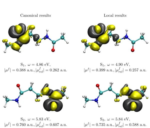
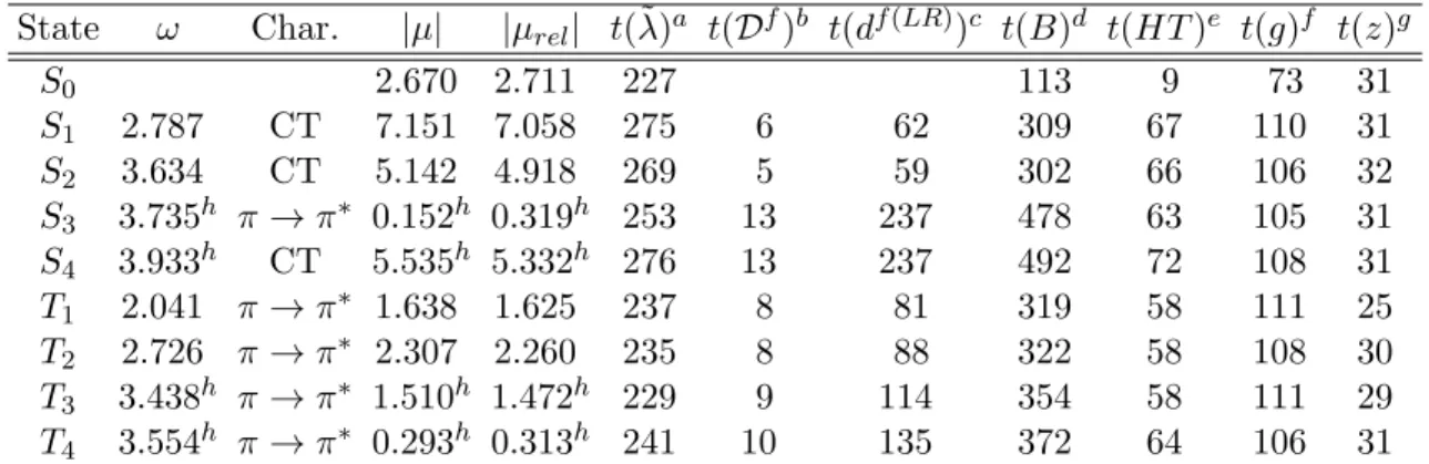
The calculation of excited state properties is very useful for the interpretation or pre- diction of the photophysical behaviour of molecules. For example, a large change in the dipole moment compared to the electronic ground state indicates a charge transfer (CT) excitation, which may enable other reaction paths than a local excitation.

In the framework of the TD-CC response theory first-order properties of individual excited states are obtained as the derivatives of the corresponding time-independent excited state Lagrangians with respect to the strength of a time-independent perturba- tion. These Lagrangians are necessary because CC is non-variational and involve the total energy of the related excited state, i.e. the ground-state energy plus the corre-

sponding excitation energy, which is within the TD-CC theory obtained as eigenvalue of the Jacobian.⁹ For an explicit inclusion of orbital-relaxation effects these Lagrangians are augmented by additional conditions related to the orbitals.

LT-DF-LCC2 excitation energies, transition moments and orbital-unrelaxed properties were implemented into theMOLPRO program package⁵⁸ earlier and enable calculations for extended molecular systems consisting of hundred or more atoms.^26–28 The method is now extended in so far that the orbitals are allowed to relax with respect to the per- turbation, i.e., orbital-relaxed first-order properties for the LT-DF-LCC2 method are presented. This is a major step on the way towards analytic gradients with respect to nuclear displacements, which will be discussed in chapter 3.

This chapter is organized as follows: First the formalism for the calculation of orbital- relaxed ground state properties is discussed in section 2.2. The approach is then applied to singlet and triplet excited states in sections 2.3 and 2.4. The orbital-relaxed densities for the ground state and excited states are discussed in detail in section 2.5. Section 2.6 comprises the results of the test calculations concerning the accuracy of the method and the results of an exemplary application. Section 2.7 summarizes the chapter.

2.2 The electronic ground state

2.2.1 The Lagrangian

The Einstein convention introduced in section 1.2.3 will be employed throughout the rest of the thesis, i.e. repeated indices are implicitly summed up. Summations are only written explicitly, if it is necessary for clarity. The formalism is derived for an orthonormal basis of molecular orbitals (MOs) and the transformation to the basis of nonorthogonal PAOs is performed a posteriori, as done in earlier work on the LMP2 gradient.⁵⁹ The MOs are expanded in an AO-basis with the metricS^AO, cf. eq. (1.13),

φp =χµCµp. (2.1)

The composite coefficient matrixC= (L|C^v) concatenates the LMO coefficient matrix L and the coefficient matrix of the canonical virtuals C^v. As introduced in chapter 1, LMOs are labeled with the indices i, j, . . ., and canonical virtuals with a, b, . . . General molecular orbitals are indexed bym, n, . . ., and PAOs by r, s, . . . In order to reduce the computational cost the density fitting approximation^15–17 is employed to decompose the

four-index integrals into three-index objects as discussed in section 1.1.2.

Properties are obtained as derivatives of the time-independent Lagrangian for the energy of the related state with respect to the strength of a time-independent perturbation. The time-independent perturbationV0, which is contained in the Hamiltonian,

H=F+V+V0 , (2.2)

is e.g. an applied electric field. In this case the corresponding property is the dipole moment. V0 consists of a Hermitian perturbation operatorXdescribing the observable, and the corresponding perturbation strengthǫX,

V0 =X

X

ǫXX=X

pq

[v0]_pqτ_q^p , (2.3)

with the matrix elements

[v0]_pq =X

X

XpqǫX . (2.4)

The general time-independent local CC2 Lagrangian for the electronic ground state without orbital relaxation, which was also used in previous work,^{25, 27, 28} reads

L^CC2₀ ^′ = E₀^CC2+ ˜λ⁰_µiΩµi. (2.5) It includes the ground state correlation energyE₀^CC2 and the amplitude equationsΩ as defined in eqs. (1.7) and (1.9). The Lagrangian is required to be stationary with respect to all parameters, i.e. the amplitudes t and multipliers ˜λ⁰. As dicussed earlier,^{25, 29} differentiation ofL^′₀with respect to the amplitudes yields the equations, which determine the multipliers,

−ηνj = ˜λ⁰_µiAµiνj , (2.6) with

ηνj = ∂E₀^CC2

∂tν_j

, (2.7)

and the JacobianA, which was defined in eq. (1.21) as Aµiνj = ∂Ωµi

∂tνj

. (2.8)

Eq. (1.7) for the CC2 ground state energy and eq. (1.9) for the CC2 amplitudes of the unperturbed system are extended by the perturbationV0, which is contained in the Hamiltonian Haccording to eq. (2.2), and explicitly arises in the second term of Ωµ2,

Ωµ2 = D

˜ µ2

Hˆ +h

F+ ˆV0,T2

i 0E

= 0 . (2.9)

Differentiating the LagrangianL^CC2₀ ^′ with respect to the perturbation strengthǫX yields the orbital-unrelaxed dipole moment of the electronic ground state, which was presented in the context of the local CC2 methods earlier.^{25, 27, 28}

The local CC2 Lagrangian for the electronic ground state including orbital relaxation reads

L^CC2₀ = L^CC2₀ ^′+z_ij^loc,0rij +z_ai⁰[f +v0]ai+x⁰_pq

C^†S^AOC−1

pq . (2.10) [f + v0]ai are the occupied-virtual matrix elements of the perturbed Fock operator [F +V0]. Compared to the orbital-unrelaxed Lagrangian L^CC2₀ ^′, L^CC2₀ contains fur- ther conditions, namely the localization, Brillouin, and orthonormality conditions. The related Lagrange multipliers are z_ij^loc,0, z_ai⁰, andx⁰_pq, respectively. The multipliers x⁰_pq re- lated to the orthogonality condition are redundant, sincex⁰ =x^0†. This will be resolved later. By choosing Pipek-Mezey localization³² the localization conditionsrij become

rij =X

A

[S_ii^A−S_jj^A]S_ij^A = 0 for all i > j, (2.11)

with the matrix S^A being defined as S_kl^A =X

µ∈A

X

ν

[LµkS_µν^AOLνl+LµlS_µν^AOLνk] . (2.12)

The summation overµ is restricted to basis functions centered on atom A.

Explicitly including the Brillouin condition in the Lagrangian L^CC2₀ leads to a different treatment of the perturbation inside the term L^CC2₀ ^′ compared to the orbital-unrelaxed

case. This will be discussed in detail in section 2.5, because it affects the density, which is needed for the calculation of the properties. Yet, it does not affect the determination of the additional Lagrange multipliers inL^CC2₀ , which will be discussed in the following section.

2.2.2 Linear z-vector equations

Differentiation of the orbital-relaxed LagrangianL^CC2₀ with respect to orbital variations yields the linear z-vector equations, from which the multipliers z⁰, z^loc,0, and x⁰ are obtained. The derivation proceeds in an analogous way as for the LMP2 gradient:^{59, 60} the variations of the orbitals in the presence of the perturbation V0 are described by the coefficient matrix

Cµp(V0) = Cµq(0)Oqp(V0), (2.13) where C(0) are the coefficients of the optimized orbitals without perturbation and the matrixO(V0) describes the rotation of the orbitals caused by the perturbationV0, with O(0) =1.

The derivative of the Lagrangian with respect to the variation of the orbitals can be partitioned into four contributions,

∂L^CC2₀

∂Opq

V0=0

= [B⁰+B(z˜ ⁰) +b(z^loc,0) + 2x⁰]pq = 0 , (2.14)

with

[B⁰]_pq =

∂

∂Opq

L^CC2₀ ^′

V0=0

, [B(z˜ ⁰)]_pq =

∂

∂Opq

z⁰_aifai

V0=0

, [b(z^loc,0)]_pi =

∂

∂Opi

z_kl^loc,0rkl

V0=0

. (2.15)

The derivation ofB⁰will be discussed in detail in the next section. The quantitiesB(z˜ ⁰) and b(z^loc,0) are identical to the quantities A, and˜ a(z^loc) given explicitly in eqs. (29)