Development of local Coupled Cluster response methods for high-spin open-shell molecules

Development of local

Coupled Cluster response methods for high-spin open-shell molecules

Dissertation

zur Erlangung des Doktorgrades der Naturwissenschaften (Dr. rer. nat.) der Fakult¨at Chemie und Pharmazie

der Universit¨at Regensburg vorgelegt von

David David

aus Tal Nasri, Haska, Syrien im Jahr 2018

Diese Arbeit wurde angeleitet von: Prof. Dr. Martin Sch¨utz

Pr¨ufungsausschuss

Vorsitzender: Prof. Dr. Hubert Motschmann

Erstgutachter: Prof. Dr. Bernhard Dick

Zweitgutachter: PD Dr. Denis Usvyat

Drittpr¨ufer: Prof. Dr. Stefan Dove

Danksagung

Ich m¨ochte mich an dieser Stelle bei allen bedanken, die zur Entstehung dieser Dissertationsarbeit beigetragen haben. Mein besonderer Dank gilt hierbei:

Dem leider inzwischen verstorbenen HerrnProf. Dr. Martin Sch¨utz f¨ur die Vergabe des sehr interessanten und anspruchsvollen Themas sowie f¨ur seine Geduld und stets kompetente Betreuung.

Herrn PD Dr. Denis Usvyat f¨ur die st¨andige Bereitschaft zur Diskussion unendlich vieler Fragen und f¨ur die ¨Ubernahme der weiteren Betreuung.

Herrn Prof. Dr. Bernhard Dick f¨ur die vielen fachlichen Ratschl¨age sowie f¨ur die freundliche ¨Ubernahme der Zweitbegutachtung.

Klaus Ziereis und Thomas Dargel f¨ur die kompetente Hilfe bei technischen Angele- genheiten.

Dr. Oliver Masur, Dr. Katrin Lederm¨uller, Dr. Stefan Loibl, Martin Christlmaier, Alexander Krach,Alexander Schinabeck, Petra Eichenseher,Dr. Marco Lorenz und Dr. Thomas Merz f¨ur eine angenehme Atmosph¨are am Arbeitskreis.

Meinem Kollegen Matthias Hinreiner f¨ur die vielf¨altigen und sehr bereichernden Diskussionen w¨ahrend der Mittagspausen.

Meinem Kollegen und FreundDr. Gero W¨alz, der mir in fachlichen als auch privaten Angelegenheiten stets zur Seite stand.

Vor allen aber meinem Herrn und Gott,Jesus Christus, der meinem Leben einen ewigen Sinn verleiht sowie meiner FrauNensina, meiner TochterMariel, meinen El- ternGaivarghis und Amira und meinen GeschwisternShamiram,Fouad und Ninab f¨ur ihre Liebe.

1. Introduction 3

2. Basic concepts 6

2.1. Coupled Cluster theory and the CC2 model . . . 6

2.2. T₁-dressed normal-ordered Hamiltonian with explicit spin . . . 11

2.3. Construction and evaluation of Coupled Cluster diagrams . . . 18

2.4. Response theory . . . 24

2.5. Density fitting . . . 29

2.6. Laplace transformation . . . 30

3. Reference wave function and localized spin orbitals 32 4. Local unrestricted CC2 ground state 35 4.1. Diagrams and working equations . . . 35

4.2. Local approximations for the ground state . . . 40

5. Local unrestricted CC2 excited states 44 5.1. Diagrams and working equations . . . 44

5.2. Local approximations for the excited state . . . 50

6. Test calculations 52 6.1. Computational behaviour and excitaion energies . . . 52

1

Contents 2 6.2. Ionisation potentials . . . 64 6.3. Electron affinities . . . 67 6.4. T1-diagnostics . . . 69

7. Summary 77

A. The second order UCC2 Lagrangian and its time average 79 B. Diagrams for the effective singles eigenvalue problem A^{ef f}_µ

1ν1U_ν1 82

C. Excitation energies of alkane radicals 84

D. Ionization potentials of alkanes 86

Open-shell molecules, radicals, play an important role in different fields of chemistry and biology. To give some examples one can think about DNA-damage in biologi- cal systems, polymerisation reactions or photocatalysis in synthetic chemistry. To understand and predict reactions in which radicals are involved needs the ability to describe the ground and excited states of these molecules. But this is still a chal- lenging task for large high-spin open-shell molecules (100 atoms). Especially if one aims at a compromise between accuracy and computational costs.

Probably the most widely used methods are Density Functional Theory (DFT) [1,2]

and time dependent (TD-)DFT. The reason is that these methods are computation- ally less demanding than correlated, wave function based, methods which go beyond Configuration Interaction Singles (CIS). Yet TD-DFT, depending on the used func- tional, may fail to produce even qualitatively reasonable results especially in case of charge transfer states [3].

Coupled Cluster (CC) theory [4–7] is well established as a wave function based method for the description of dynamical correlation effects. The restriction of the cluster operator to singles and doubles (CCSD) has also been used to describe high-spin open-shell systems along with a single-reference determinant, but often a straight forward usage of unrestricted spin-orbital formalism has been avoided [8–11].

The main reasons are spin contamination and computational costs.

However, if a restricted open-shell Hartree-Fock (ROHF) reference determinant is

3

4 chosen instead of unrestricted Hartree-Fock (UHF), the excitation energies despite the remaining spin contamination, which arises from not solving the CC spin equa- tions, are in good agreement (absolute error < 0.1 eV) with the Multi-Reference Configuration Interaction (MR-CI) results for a set of diatomic molecules described in reference [12].

CCSD scales asO(N⁶) with molecular size N and a straight forward, unrestricted spin-orbital formulation, even if based on a ROHF reference implies a computational cost factor of 3 compared to the corresponding closed-shell calculation [13].

Thus the search for reduction of computational costs along with a straight for- ward implementation using unrestricted spin-orbital formulation, but maintaining the ROHF reference and reaching a reasonable accuracy, lead to the work presented here.

Firstly, one chooses the approximate CC2 Model [14] which scales as O(N⁵) with molecular size N instead of CCSD (O(N⁶)).

Secondly, one starts with a ROHF reference and generates out of it the semi- canonical spin orbitals [15]. The occupied ones are transformed to localized spin orbitals and atomic orbitals are projected to the virtuals as proposed by Pulay [16].

Thirdly, Density Fitting (DF) approximation [17–19], for reduction of the prefactor of the scaling behaviour, and local approximations in order to reach a lower order scaling of CC2, are applied. Note that a canonical, non local, implementation of CC2 based only on the DF approximation for high-spin open-shell molecules is avail- able in theTURBOMOLE package [20].

Fourthly, inspired by the work of D. Kats and M. Sch¨utz [21], the laplace-transform (LT) trick is used to enable a multistate CC2 response method along with local approximations in analogy to what is already available in MOLPRO [22] for closed- shell molecules. So the new method will be called LT−DF−LUCC2 (laplace- transformed density fitted local unrestricted CC2).

At the beginning basic concepts which are necessary for the development of the presented method are introduced. It follows the choice of the reference wave func- tion and the description of local spin orbitals. Then the derivation of the working equations for the ground and excited state of high-spin open-shell molecules as well as corresponding local approximations are outlined. Finally the application of that method to calculate excitation energies, ionization potentials and electron affinities is demonstrated.

2. Basic concepts

In this chapter several basic concepts are introduced for the understanding of the method presented in this thesis. As the method is based on Coupled Cluster (CC) theory, response theory, construction and evaluation of CC diagrams, density fitting and Laplace transformation, these concepts are explained.

2.1. Coupled Cluster theory and the CC2 model

It is well known that the movement of two electrons with opposite spin is not corre- lated within the use of a single Slater Determinant (SD). To capture this dynamic electron correlation, or to describe the coulomb hole correctly, many theoretical methods have been developed. Among the wave function based methods like Config- uration Interaction (CI) or perturbation theory along with the Møller-Plesset (MP) partitioning of the electronic Hamiltonian, the Coupled Cluster (CC) theory [4–7]

is very successful and widely used.

A SD which contains occupied Hartree Fock spin orbitals, is usually used as a refer- ence determinant to generate the CC wave function |CCi through the exponential ansatz.

|CCi= exp(T)|Φ₀i (2.1)

6

In equation (2.1), |Φ₀i symbolizes the reference determinant and T is the total cluster operator, which is defined as

T=

Nelec

X

i=1

T_i. (2.2)

Here each summand T_i implies replacement of i occupied spin orbitals by virtual ones. This replacement is often referred to as generating excited determinants. Each cluster operator T_i contains products of amplitudest_µi and corresponding excitation operatorsτ_µi to generate all possible i-fold excited determinants. For example, the singles and doubles cluster operators are defined as

T₁ =X

µ1

t_µ1τ_µ1 =X

IA

t^I_Aa^†_Aa_I

T2 =X

µ2

tµ2τµ2 = 1 4

X

IJ AB

t^IJ_ABa^†_Aa^†_BaJaI (2.3) The capital letters I, J, ...and A, B, ... represent occupied and virtual spin orbitals, respectively, while the explicit spin (α or β) of the corresponding orbital is not yet specified. The second quantization operatora_I annihilates the occupied spin orbital I from|Φ₀i and a^†_A introduces the virtual spin orbital A in it. Thusa^†_A and a_I are referred to as the creation and annihilation operators, respectively. The factor ¹₄ is included to avoid double counting of spin orbital pairs.

Due to the exponential ansatz, even if the cluster operator is truncated, one has formally all possible higher excitations. The products of amplitudes are referred to as disconnected cluster amplitudes. Irrespective of the truncation level ofT, the CC models are size consistent. That means, that the total energy of a system composed of noninteracting subsystems is the same as the sum of the energies of each subsystem calculated separately. This is fulfilled because the exponential ansatz makes the CC wave function multiplicative separable and the corresponding expectation values of the Hamiltonians additive. But in cases where the reference method fails to be size

2.1 Coupled Cluster theory and the CC2 model 8 consistent, also the correlated method will not be. In general for the CC models, the mathematically stronger requirement that the energy scales correctly with the number of the correlated electrons is fulfilled. This feature is referred to as size extensivity.

For the calculation of the CC energy a projective technique is used instead of the usual quantum mechanical expectation value equation.

E =hΦ₀|exp(−T)Hexp(T)|Φ₀i=hΦ₀|H|Φ¯ ₀i (2.4) The reason for that is that exp(T)^† would act on the left as an excitation operator giving rise to much more matrix elements of the Hamilton operator H than in equation (2.4). The Hamiltonian can be written in second quantized form as

H=X

P Q

h_{P Q}a^†_Pa_Q+1 4

X

P QRS

hP Q||RSia^†_Pa^†_Qa_Sa_R. (2.5) With the following definition of the one electron integral,

h_{P Q} = Z

ψ^∗_P(x₁)h(r₁)ψ_Q(x₁)dx₁, (2.6) which describes the kinetic energy of a single electron with three space and one spin coordinate hidden in x₁ as well as the coulomb attraction between an electron and all nuclei. The antisymmetrized two electron integrals are defined as

hP Q||RSi=hP Q|RSi − hP Q|SRi hP Q|RSi=

Z

ψ_P^∗(x₁)ψ_Q^∗(x₂) 1 r12

ψ_R(x₁)ψ_S(x₂)dx₁dx₂ (2.7) P QRS...indicate general spin orbitals which can be either occupied or virtual.

Use of the similarity transformed Hamiltonian ¯His justified by the fact that, in case of no truncation, its eigenvalues represent the complete eigenvalue spectrum of the hermitian Hamilton operatorH. ¯Hcan be written in the Baker-Campbell-Hausdorff (BCH) expansion,

H¯ =H+ [H,T] + 1

2![[H,T],T] + 1

3![[[H,T],T],T] + 1

4![[[[H,T],T],T],T], (2.8)

which terminates exactly after the fifth term, because each commutator reduces the number of the general creation and annihilation operators of the Hamiltonian by one. Thus after the fifth term only creation and annihilation operator strings with either occupied or virtual spin orbital index remain and these commute. Equation (2.4) is called the linked CC energy equation. For the determination of the CC amplitudes, the so-called linked CC amplitudes equations have to be solved.

Ω_µi =hµ_i|exp(−T)Hexp(T)|Φ₀i= 0^! (2.9) While |µ_ii represents all possilbe i-fold excited determinants. Solving the CC am- plitudes equations iteratively, yields the corresponding amplitudest_µi for which the residuums vector Ω_µi becomes zero. These amplitudes determine the final CC en- ergy (2.4).

By restriction of the Cluster operator T to singles and doubles excitations one ar- rives at the well known CCSD model. The singles and doubles amplitudes equations for that model can be written in a compact form as

Ω_µ1 =hµ₁|Hˆ + [ ˆH,T₂]|Φ₀i (2.10) and

Ω_µ2 =hµ₂|Hˆ + [ ˆH,T₂] + 1

2![[ ˆH,T₂],T₂]|Φ₀i, (2.11) where the T₁-dressed (similarity transformed) Hamilton operator ˆH is defined as

Hˆ = exp(−T1)Hexp(T1). (2.12) For the singles amplitudes equation (2.10), the expansion series of exp(−T₂) ˆHexp(T₂) terminates after the second term, because the action of further products of T2 can not be compensated by the Hamiltonian in order that only singly excited determi- nants remain on the bra side. In an analogous manner of reasoning the commutator

2.1 Coupled Cluster theory and the CC2 model 10 series in the doubles equation (2.11) terminates after the third term.

If the Hamiltonian is partitioned into a Fock operatorFand a fluctuation potential operator W, describing the difference between the real electron-electron repulsion and the Fock potential, the CC2 model [14] is obtained from CCSD by simplifying the doubles equation (2.11) as

Ω_µ2 =hµ₂|Hˆ + [F,T₂]|Φ₀i. (2.13) In closed-shell cases the Fock operator is usually regarded to be of zeroth order (F^[0]) in the fluctuation potential, W^[1], which it self is of first order. The fact that off-diagonal elements of the Fock operator for closed-shell molecules are zero, gives a leading contribution of the singles amplitudes of second order [24]. And only the first order doubles amplitudes contribute to the second order energy correction.

However, in open-shell cases off-diagonal Fock elements are not zero and thus par- titioning the Hamiltonian as

H=F^[0]+F^[1]+W^[1] (2.14)

leads to a contribution of the singles amplitudes in first order. F^[0] andF^[1]represent the diagonal and off-diagonal parts of the Fock operator, respectively. Nevertheless, in CC2 the singles are formally assumed to be of zeroth order to obtain a doubles equation (2.13) which is correct only to first order as in the closed-shell case [14].

Finally it is this form of the doubles equation which enables building the so-called

”effective singles eigenvalue problem” which will be explained in detail in chapter 5.

2.2. T

-dressed normal-ordered Hamiltonian with explicit spin

Before examination of the effect of T₁-dressing and normal-ordering on the Hamilton operator (2.5), it is given in its explicit spin form as

H=X

pαqα

h_pαqαa^†_pαa_qα+X

p_βq_β

h_pβqβa^†_pβa_qβ

+1 4

X

pαqαrαsα

hpαqα||rαsαia^†_pαa^†_qαasαarα

+1 4

X

pβqβrβsβ

hp_βq_β||r_βs_βia^†_p

βa^†_q

βa_sβa_rβ

+ X

pαqβrαsβ

hp_αq_β|r_αs_βia^†_pαa^†_q

βa_sβa_rα . (2.15) The one and two electron integrals entering the equation above have been introduced in the previous section in equations (2.6) and (2.7). The sole difference is that the spin of the orbitals is given explicitly for valid spin combinations in equation (2.15).

One can express the singles cluster operator T₁ with explicit spin as T₁ =X

iαaα

tⁱ_a^α_αa^†_aαa_iα +X

iβaβ

tⁱa^ββa^†_a

βa_iβ . (2.16)

Similarity transformation of equation (2.15) leads to the following expression Hˆ =X

pαqα

h_pαqαexp(−T₁)a^†_pαa_qαexp(T₁) +X

pβqβ

h_pβqβexp(−T₁)a^†_p

βa_qβexp(T₁) +1

4 X

pαqαrαsα

hp_αq_α||r_αs_αiexp(−T₁)a^†_pαa^†_qαa_sαa_rαexp(T₁) +1

4 X

pβqβrβsβ

hp_βq_β||r_βs_βiexp(−T₁)a^†_p

βa^†_q

βa_sβa_rβexp(T₁)

+ X

pαqβrαsβ

hp_αq_β|r_αs_βiexp(−T₁)a^†_pαa^†_q

βa_sβa_rαexp(T₁) . (2.17)

2.2 T₁-dressed normal-ordered Hamiltonian with explicit spin 12 For the one-electron part with σ spin, (σ =α orβ), one gets

X

pσqσ

h_pσqσexp(−T₁)a^†_p

σa_qσexp(T₁) =

=X

pσqσ

h_pσqσexp(−T₁)a^†_pσexp(T₁) exp(−T₁)

| {z }

=1

a_qσexp(T₁) . (2.18)

Using the BCH expansion, like in equation (2.8), and applying the anticommutation relations

[a^†_pσ, a^†_qτ]₊ = 0, [a_pσ, a_qτ]₊= 0, [a^†_pσ, a_qτ]₊=δ_pσqτδ_στ, (2.19) for the creation and annihilation operators, one obtains

ˆ

a^†_pσ = exp(−T₁)a^†_pσexp(T₁) =a^†_pσ −X

iσaσ

tⁱ_a^σ_σa^†_aσδ_pσiσ (2.20)

and

ˆ

a_qσ = exp(−T₁)a_qσexp(T₁) =a_qσ +X

iσaσ

tⁱ_a^σ

σa_iσδ_qσaσ . (2.21) One has to note that for a set of non-orthogonal orbitals the anticommutator between a creation and an annihilation operator becomes

[a^†_pσ, a_qτ]₊=S_pσqτδ_στ (2.22) whereS_pσqτ is the overlap integral between the spin orbitalsp_σ and q_τ. But the use of a biorthogonal basis yields exactly the same relationships as given in equation (2.19) [25]. The matrices X^σ and Y^σ,

X^σ =1−t₁^σ with [t₁]_pσqσ ={t^q_p^σ_σ, if p_σ ∈virt. & q_σ ∈occ. else 0

Y^σ =1+ (t₁^σ)^T , (2.23)

are introduced and have for an example with two occupied and two virtual spin orbitals the following structure.

X^σ =





















i_σ j_σ a_σ b_σ

i_σ 1 0 0 0

j_σ 0 1 0 0

a_σ −tⁱ_a^σ_σ −t^j_a^σ_σ 1 0 b_σ −tⁱ_b^σ

σ −t^j_b^σ

σ 0 1





















;Y^σ =





















i_σ j_σ a_σ b_σ i_σ 1 0 tⁱ_a^σ_σ tⁱ_b^σ

σ

j_σ 0 1 t^j_a^σ_σ t^j_b^σ

σ

a_σ 0 0 1 0

b_σ 0 0 0 1





















(2.24)

σ can be eitherα orβ. In case of using PAOs for the virtual space, each element of the occupied-virtual block ofY^σhas to be multiplied with the corresponding element of the PAO-overlap matrix. The similarity transformed creation and annihilation operators can be written as

ˆ

a^†_pσ =X

rσ

a^†_rσ[X^σ]_rσpσ =X

rσ

a^†_rσX_rσpσ (2.25)

and

ˆ

a_qσ =X

sσ

a_sσ[Y^σ]_sσqσ =X

sσ

a_sσY_sσqσ. (2.26) From equations (2.20) and (2.21) as well as from the structure of X^σ and Y^σ one can immediately see that ˆa^†_pσ = a^†_pσ if pσ ∈ virtual and ˆaqσ = aqσ if qσ ∈ occupied space. If equations (2.25) and (2.26) are used, the one electron part of the dressed Hamiltonian in second quantized form can be written as

X

pσqσ

h_pσqσˆa^†_p

σˆa_qσ =X

pσqσ

h_pσqσ X

rσ

a^†_r

σX_rσpσX

sσ

a_sσY_sσqσ

rσ↔pσ

sσ=↔qσ

X

pσqσ

X

rσsσ

X_pσrσh_rσsσY_qσsσa^†_pσa_qσ

=X

pσqσ

ˆh_pσqσa^†_pσa_qσ . (2.27)

2.2 T₁-dressed normal-ordered Hamiltonian with explicit spin 14 It follows again from the structure of X^σ and Y^σ that ˆh_iσaσ = h_iσaσ and that ˆhpσqσ 6= ˆhqσpσ. Analogously theααand theββ two-electron part of the Hamiltonian can be formulated as

1 4

X

pσqσrσsσ

hp_σq_σ||r_σs_σiaˆ^†_p

σaˆ^†_q

σaˆ_sσˆa_rσ

=1 4

X

pσqσrσsσ

hp_σq_σ||r_σs_σiX

tσ

a^†_tσX_tσpσ X

uσ

a^†_uσX_uσqσ X

vσ

a_vσY_vσsσX

wσ

a_wσY_wσrσ

=1 4

X

pσqσrσsσ

X

tσuσvσwσ

ht_σu_σ||w_σv_σiX_pσtσX_qσuσY_sσvσY_rσwσa^†_pσa^†_qσa_sσa_rσ

=1 4

X

pσqσrσsσ

hp_σq_σ||rˆ _σs_σia^†_pσa^†_qσa_sσa_rσ (2.28)

The dressed two-electron integrals hp_σq_σ||rˆ _σs_σi = hp_σq_σˆ|r_σs_σi − hp_σq_σˆ|s_σr_σi have only the permutational symmetry of the electrons, i. e. hpσqσˆ|rσsσi =hqσpσˆ|sσrσi.

Applying the same strategy for expressing theαβ part of the two-electron part and putting together the remaining parts after dressing, leads to the following equation for the dressed Hamilton operator with explicit spin.

Hˆ =X

pαqα

ˆh_pαqαa^†_p

αa_qα +1 4

X

pαqαrαsα

hp_αq_αˆ||r_αs_αia^†_p

αa^†_q

αa_sαa_rα

+X

pβqβ

ˆh_pβqβa^†_p

βa_qβ +1 4

X

pβqβrβsβ

hp_βq_βˆ||r_βs_βia^†_p

βa^†_q

βa_sβa_rβ (2.29)

+ X

pαqβrαsβ

hp_αq_βˆ|r_αs_βia^†_pαa^†_q

βa_sβa_rα

In the final analysis it can be clearly seen that the effect of dressing is carried over to the integrals and the creation and annihilation operators are retained in their undressed form. Hence the normal-ordering of the dressed Hamiltonian can be per- formed in exactly the same way as for the undressed operator.

A normal-ordered string of operators is one in which all annihilation operators stand

to the right of the creation operators. This can be achieved by using the anticom- mutation relations (2.19).

A more convenient way to normal-order any string of creation and annihilation operators is the application of Wick’s theorem which states that every string can be normal-ordered by writing it as linear combinations of pairwise contractions of operators, i.e.

ABC . . . IJ K ={ABC . . . IJ K}v+X

s

{ABC . . . IJ K}v

+X

d

{ABC . . . IJ K}v+. . . (2.30) The first term in the equation above denotes the totally normal-ordered string with respect to the true vacuum state (v). The first sum is over all possible single pair contractions and the second one over all possible double pair contractions.

The generalised Wicks theorem states that products of normal-ordered operator strings can be normal-ordered by writing the complete string as a sum of the normal-ordered string and the pairwise contractions between operators of the in- volved normal-ordered strings and no contractions within a normal-ordered string itself.

{ABCD . . .}v{IJ KL . . .}v ={ABCD . . . IJ KL . . .}v+X

s

{ABCD . . . IJ KL . . .}

+X

d

{ABCD . . . IJ KL . . .}+... (2.31) A contraction between two operators is defined as the pair it self minus the normal- ordered form of the pair.

AB=AB− {AB}v (2.32)

For each permutation of two operators one has to multiply the operator string with

−1. If one examines the four possible pairs of creation and annihilation operators

2.2 T₁-dressed normal-ordered Hamiltonian with explicit spin 16 (same spin) for a contraction, one gets

a_pσa^†_qσ =a_pσa^†_qσ − {a_pσa^†_qσ}_v=a_pσa^†_qσ +a^†_qσa_pσ =δ_pσqσ (2.33) as the only nonzero combination.

As any matrix element hψ₂|O|ψ₁i can be written as h|(A₂)^†OA₁|i with |ψ₁i=A₁|i and |ψ₂i =A₂|i, where |i is the true vacuum state, only fully contracted terms of the string (A₂)^†OA₁ give nonzero results.

However, it is more convenient to work with a slater determinant (SD) as a reference state, (also called the Fermi vacuum) than the true vacuum state. For the use of a SD as a reference state a so-called particle hole formalism has to be introduced and creation and annihilation operators with respect to this reference state have to be defined. The quasi-particle creation operators are

a_iσ and a^†_a

σ , (2.34)

becauseaiσ working on a SD creates a hole (the spin orbital iσ is occupied) anda^†_aσ creates a particle. And the quasi-particle annihilation operators are

a^†_i

σ and a_aσ , (2.35)

because they annihilate possible holes and particles.

With the quasi-particle operators a normal-ordered string is one, in which all quasi- particle annihilation operators stand to the right of the quasi-particle creation oper- ators. When all eight possible combinations of quasi-particle creation and annihila- tion operators (same spin) are examined, the only two pairs giving a nonzero result after performing the contraction are

a_aσa^†_b

σ =a_aσa^†_b

σ − {a_aσa^†_b

σ}=a_aσa^†_b

σ +a^†_b

σa_aσ =δ_aσbσ (2.36) and

a^†_i

σa_jσ =a^†_i

σa_jσ − {a^†_i

σa_jσ}=a^†_i

σa_jσ +a_jσa^†_i

σ =δ_iσjσ . (2.37)

Now it is straight forward to get the normal-order of the dressed Hamilton operator (2.29) with respect to the Fermi vacuum. The one-electron part for example can be normal-ordered as

X

pσqσ

ˆh_pσqσa^†_pσa_qσ =X

pσqσ

hˆ_pσqσ{a^†_pσa_qσ}+X

pσqσ

ˆh_pσqσ{a^†_pσa_qσ}

=X

pσqσ

hˆpσqσ{a^†_pσaqσ}+X

pσqσ

ˆhpσqσδpσqσδpσ∈iσ

=X

pσqσ

hˆ_pσqσ{a^†_pσa_qσ}+X

iσ

ˆh_iσiσ . (2.38) Wicks theorem (2.30) and the contraction of equation (2.37) have been used. Normal- ordering of the remaining parts of the dressed Hamilton operator and considering the particle permutational symmetry of the dressed two-electron integrals leads to Hˆ =X

pαqα

hˆ_pαqα+X

iα

hi_αp_α||iˆ _αq_αi+X

iβ

hi_βp_αˆ|i_βq_αi a^†_p

αa_qα

+X

pβqβ

ˆh_pβqβ +X

i_β

hi_βp_β||iˆ _βq_βi+X

iα

hi_αp_βˆ|i_αq_βi a^†_p

βa_qβ +1

4 X

pαqαrαsα

hpαqαˆ||rαsαi

a^†_pαa^†_qαasαarα

+1 4

X

pβqβrβsβ

hp_βq_β||rˆ _βs_βi a^†_p

βa^†_q

βa_sβa_rβ

+ X

pαqβrαsβ

hp_αq_βˆ|r_αs_βi a^†_pαa^†_q

βa_sβa_rα

+X

iα

hˆ_iαiα +1 2

X

iαjα

hi_αj_αˆ||i_αj_αi+X

iβ

ˆh_iβiβ +1 2

X

iβjβ

hi_βj_βˆ||i_βj_βi+X

iαjβ

hi_αj_βˆ|i_αj_βi

=ˆF^α_N+ ˆF^β_N+ ˆV^αα_N + ˆV^ββ_N + ˆV^αβ_N +hΦ₀|H|Φˆ ₀i

= ˆH_N+hΦ₀|H|Φˆ ₀i . (2.39)

The normal-ordering of the non similarity transformed Hamiltonian has been demon- strated in detail in reference [26]. The general statement that the normal-order of an operator is the same as the operator itself minus its expectation value holds also

2.3 Construction and evaluation of Coupled Cluster diagrams 18 in the case of the dressed Hamiltonian.

Hˆ_N = ˆF^α_N+ ˆF^β_N+ ˆV^αα_N + ˆV^ββ_N + ˆV_N^αβ (2.40) The CC2 singles (2.10) and doubles (2.13) amplitudes equations remain unchanged wether one uses the non normal-ordered or the normal-ordered dressed Hamilton operator, as will be shown later. But it is much easier to work with the already normal-ordered strings of the dressed Hamiltonian when analyzing any matrix ele- ments.

However, looking at the energy equation of CC2, E_CC2 =hΦ₀|exp(−T₂) ˆHexp(T₂)|Φ₀i

=hΦ₀|exp(−T₂)( ˆH_N+hΦ₀|H|Φˆ ₀i) exp(T₂)|Φ₀i

=hΦ₀|exp(−T₂) ˆH_Nexp(T₂)|Φ₀i+hΦ₀|H|Φˆ ₀i , (2.41) one can conclude that the expression

hΦ₀|exp(−T₂) ˆH_Nexp(T₂)|Φ₀i=E_CC2− hΦ₀|H|Φˆ ₀i (2.42) represents a sort of correlation energy. But one has to be careful, becausehΦ₀|H|Φˆ ₀i is not the Hartree-Fock energy hΦ0|H|Φ0i. That is the reason why the CC2 corre- lation energy is calculated using the non-dressed normal-ordered Hamilton operator HN instead of ˆHN.

2.3. Construction and evaluation of Coupled Cluster diagrams

Using Wicks theorem as introduced in equations (2.30) and (2.31), it is straight forward to derive working equations from the CC2 amplitudes equations (2.10) and

(2.13). But this is a rather tedious way compared to the diagrammatic technique. In reference [26] the rules for construction and evaluation of Coupled Cluster diagrams have been shown for the case of orthogonal spin orbitals. Here the construction and evaluation of diagrams within the use of the T1-dressed normal-ordered Hamiltonian (2.40) and the non-orthogonal PAOs will be discussed.

For the construction of CC diagrams the quasi particle-hole formalism and the cor- responding quasi creation and annihilation operators as introduced in section 2.2 are needed. A so-called hole line is one directed downward and symbolizes an occu- pied orbital in the reference determinant. The particle line is directed upward and symbolizes a virtual orbital.

The Hamilton operator fragments are described by horizontal lines which are dashed.

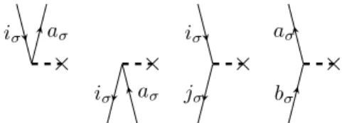
Fˆ^σ_N is an one-electron operator an thus has one vertice on which creation and anni- hilation operators can act.

×

iσ aσ

×

iσ a_σ

×

iσ

jσ

×

aσ

b_σ

Figure 2.1.: ˆF^σ_N fragments with excitation levels +1,−1, 0 and 0 (from left to right)

In figure 2.1 the four possible ˆF^σ_N fragments are shown, where σ can be either α or β. This yields in total eight diagrams. In the most left fragment two quasi creation operators are symbolized by two lines above the horizontal operator line (also called interaction line). The excitation level is calculated by subtracting the number of quasi particle lines under the interaction line (annihilation operator lines) from the quasi particle lines above it (creation operator lines) and dividing the result by two. One gets, e.g. for the most right fragment of figure 2.1 an excitation level of

(1−1)

2 = 0. Also the non-dressed Fock operator which appears in the CC2 doubles equation (2.13) will be represented by the same diagrams. It will be clear from

2.3 Construction and evaluation of Coupled Cluster diagrams 20 the context if it is a dressed or a non-dressed fragment of the Hamiltonian. A line pointing toward a vertice is called incoming line and when pointing away it is called outgoing line. Both lines on a vertice have to correspond to the same spin.

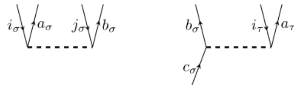
For the two-electron operator ˆV^σσ_N or ˆV^στ_N (withσ=αandτ =β or vice versa) there are two vertices and correspondingly two incoming and two outgoing lines. Diagrams for a ˆV_N^σσ and ˆV^στ_N fragment with an excitation level of +2 and +1, respectively, are shown in figure 2.2.

iσ aσ j_σ bσ

c_σ

bσ iτ aτ

Figure 2.2.: ˆV^σσ_N and ˆV^στ_N fragments with excitation levels +2 and +1

The amplitudes of the cluster operators are illustrated by solid horizontal lines.

As the cluster operators contain only quasi creation operators, they are already normal-ordered with respect to Fermi vacuum. The α or β singles cluster operator T^σ₁ =P

iσaσ tⁱ_a^σ_σ{a^†_aσa_iσ} corresponds to an excitation level of +1 and is represented as shown in figure 2.3.

i_σ aσ

Figure 2.3.: Diagrammatic representation of T^σ₁

Doubles cluster operators, T^σσ₂ = 1

4 X

iσaσjσbσ

tⁱ_a^σjσ

σbσ{a^†_aσa^†_b

σa_jσa_iσ} or

T^στ₂ = X

iσaσjτbτ

tⁱ_a^σjτ

σbτ{a^†_aσa^†_b

τa_jτa_iσ}

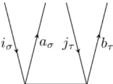
whereσ and τ can be eitherα orβ, correspond to an excitation level of +2. T^στ₂ is diagrammatically represented as drawn in figure 2.4.

iσ aσ j_τ bτ

Figure 2.4.: Diagrammatic representation of T^στ₂

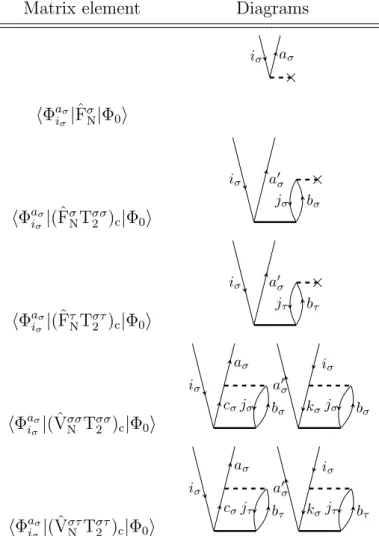
Having these elements at hand, one can draw diagrams corresponding to matrix elements in a simple way. For example the matrix elementhΦ^a_iσ^σ|Fˆ^σ_N|Φ₀iis represented by the diagram in figure 2.5.

×

i_σ aσ

Figure 2.5.: Diagrammatic representation of hΦ^a_i^σ

σ|Fˆ^σ_N|Φ₀i

The reference determinant is represented by the empty space under the horizontal line corresponding to ˆF^σ_N and the singly excited determinanthΦ^a_iσ^σ|by the two exter- nal lines. So on the top of the diagram is the bra-side and on the bottom the ket-side of the matrix element. In between are the fragments of the Hamilton operator. In figure 2.5 one has to use the ˆF^σ_N fragment with the excitation level +1 to match the excitation level on the bra-side. The agreement of the excitation level of the bra-side

2.3 Construction and evaluation of Coupled Cluster diagrams 22 and the parts of the Hamiltonian working on the ket-side has to be fulfilled when representing matrix elements by CC diagrams.

As a further example the diagram for the matrix elementhΦ₀|( ˆV^σσ_N T^σσ₂ )_c|Φ₀iis shown in figure 2.6. There one has only internal lines, i.e. lines which start and end at

iσ aσ j_σ bσ

Figure 2.6.: Diagrammatic representation ofhΦ0|( ˆV^σσ_N T^σσ₂ )c|Φ0i

operator interaction lines. No external lines like in figure 2.5 occur, because the overall excitation level of the diagram is zero.

The subscript c indicates that the cluster operators standing to the right of the Hamilton operator fragment have to be connected at least once to it. This result is obtained when carrying out Wicks theorem on the commutators introduced by the Baker-Campbell-Hausdorff expansion of the T1-dressed and normal-ordered Hamil- tonian of equation (2.40).

The evaluation of CC diagrams is carried out according to the following rules.

• The sign is calculated as (−1)^l+h, with l and h as abbreviations for loops and hole lines in a diagram.

• Each pair of equivalent lines, which start and end at the same operator inter- action line and have the same spin, like (i_σ, j_σ) or (a_σ, b_σ) in figure 2.6, yields a prefactor of ¹₂.

• A summation is carried over each index of an internal line.

• The Fock operator fragment, e.g. ˆF^σ_N, contributes an integralhout|fˆ|ini, where

”out” is the outgoing and ”in” the incoming line on the vertice of the operator.

And a cluster operator interaction line contributes the corresponding ampli-

tude to the expression, e.g. tⁱ_a^σjσ

σbσ from the diagram in figure 2.6. The indexes are taken first from the left and then from the right vertice of the amplitude.

• The two-electron operator ˆV_N^σσ contributes a dressed integral of the form hl-out r-outˆ||l-in r-ini, where l and r mean the left and right vertice of the operator. But ˆV^στ_N, with σ = α and τ = β or vice versa, contributes the integral hl-out r-outˆ|l-in r-ini. Whereas in chemist notation the corresponding integrals would be (l-out l-inˆ|r-out r-in)− (l-out r-inˆ|r-out l-in) for ˆV^σσ_N and (l-out l-inˆ|r-out r-in) for ˆV_N^στ.

• If a diagram contains n equivalent vertices, the algebraic expression is multi- plied by a factor of _n!¹. For example the diagrammatic representation of the matrix element hΦ₀|(V^αα_N T^α₁T^α₁)_c|Φ₀i, which appears in the CC2 energy equa- tion, contains two equivalent vertices (figure 2.7 ), because both T^α₁ fragments are connected the same way to V^αα_N and both vertices have incoming and out- going lines of the same spin. According to this rule the representation of the matrix element hΦ₀|(V^αβ_N T^α₁T^β₁)_c|Φ₀i does not contain equivalent vertices.

iσ a_σ jσ bσ

Figure 2.7.: Diagrammatic representation ofhΦ0|(V_N^ααT^α₁T^α₁)c|Φ0i

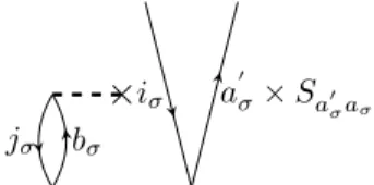
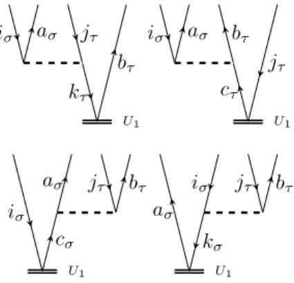
• For each external outgoing line of an amplitude vertice, i.e. the line is not connected to a fragment of the Hamilton operator, the corresponding ampli- tude has to be multiplied by the PAO overlap matrix. This rule has to be applied for example when evaluating the matrix element hΦ^a_iσ^σ|(ˆF^σ_NT^σσ₂ )_c|Φ₀i.

One possible corresponding diagrammatic representation is shown in figure 2.8.