Development of local coupled cluster response methods for vertical Ionization Potentials

coupled cluster response methods for vertical Ionization Potentials

Dissertation

zur Erlangung des Doktorgrades der Naturwissenschaften (Dr. rer. nat.) der Fakultät Chemie und Pharmazie

der Universität Regensburg vorgelegt von

Gero Wälz

aus Ingolstadt

im Jahr 2017

Prüfungsausschuss

Vorsitzender: Prof. Dr. Arno Pfitzner

Erstgutachter: Prof. Dr. Martin Schütz

Zweitgutachter: PD Dr. Denis Usvyat

Drittprüfer: Prof. Dr. Ferdinand Evers

Ersatzprüfer: Prof. Dr. Alkwin Slenczka

Ein herzliches Dankeschön geht an alle, die mich in den letzten Jahren un- terstützt haben und ohne die die Fertigstellung einer solchen Arbeit schwer vorstellbar ist. Im Besonderen sind das:

Prof. Dr. Martin Schütz, der mich fachlich unterstützt hat und mir immer wieder das Vertrauen geschenkt hat dieser Aufgabe gewachsen zu sein.

Dr. Denis Usvyat für seine ständige Bereitschaft jede Frage stets gut gelaunt zu beantworten.

Dr. Tatiana Korona, die mir den Start dieser Arbeit mit ihrem kanonischen IP-CC2 Programm sehr erleichtert hat.

Den ehemaligen Mitarbeitern des Arbeitskreises, Dr. Daniel Kats und Dr.

Keyarash Sadeghian, die für Fragen weiterhin zur Verfügung standen.

Dr. Stefan Loibl, für die schöne Zeit im Büro und in der Freizeit.

Meinen Kollegen Katrin Ledermüller, Oliver Masur, Martin Christlmaier und Alexander Krach für ihre Bereitschaft aufeinander einzugehen und mit ihrem eigenen Wissen weiterzuhelfen.

Meinen Kollegen Thomas Merz und Matthias Hinreiner für die vielen gemein- sam verbrachten Mittagsstunden und Kaffeerunden, sowie die exzellente Ver- sorgung mit Kuchen.

Meinem Freund und Kollegen David David, im Besonderen für die etlichen Glaubensgespräche.

Meinen Eltern Marita und Michael gebührt der Dank nicht nur für die letzten

Jahre, sondern für ihre Liebe und Unterstützung mein Leben lang.

Chapter 2 und Section 3.2

G. Wälz, D. Usvyat, T. Korona and M. Schütz

"A hierarchy of local coupled cluster singles and doubles response methods for ionization potentials"

The Journal of Chemical Physics

144, 084117 (2016), doi: 10.1063/1.4942234

1. Introduction 3

1.1. Coupled cluster methods . . . . 4

1.2. Approximations . . . . 8

1.2.1. Local ansatz . . . . 8

1.2.2. Density fitting . . . 10

1.2.3. Laplace transformation . . . 11

1.3. Diagrammatic techniques . . . 12

2. Hierarchy of local coupled cluster ionization potentials 15 2.1. Introduction . . . 15

2.2. Response theory for ionized states . . . 16

2.3. Approximate coupled cluster model CC2 . . . 21

2.4. Additional higher order diagrams . . . 26

2.4.1. IP-CCSD[1]

. . . 27

2.4.2. IP-CCSD[2]

. . . 28

2.4.3. IP-CCSD[f]

. . . 29

2.4.4. Local approximations . . . 31

2.5. Test calculations . . . 33

2.5.1. Accuracy of the IP-CCSD[k]

hierarchy . . . 34

2.5.2. Accuracy of local approximations . . . 37

2.5.3. Calculations on D21L6 . . . 39

3. Hierarchy extension to the five-half excitation space 43 3.1. Introduction . . . 43

3.2. Excitation energies of radicals . . . 44

1

3.3. IP-CC3

theory . . . 48 3.3.1. Co- and contravariant configuration state functions . . . 48 3.3.2. IP-CC3

Jacobian . . . 49 3.3.3. Local approximations . . . 55

4. Local coupled cluster electron affinities 57

4.1. Introduction . . . 57 4.2. Theory . . . 58

5. Summary 62

A. Supplementary information for test calculations 64

B. Coupled Cluster diagrams 77

Bibliography 81

The term theoretical chemistry sounds at the first glance contradictory. Com- monly, when people think of chemistry, they tend to imagine something hap- pening in a laboratory where some kind of synthesis is performed. And, it is true, chemistry today is still a lot of synthesizing. But chemistry contains a lot more than that. Chemistry is also examination of substances with a variety of methods, e.g. with different forms of spectroscopy. Or, coming back to a theoretical chemistry, simulation of chemical processes and prediction of prop- erties. A simulation can, for example, reveal that a planned synthesis does not lead to the desired product. Or it can be used to verify experimental results.

The combination of experimental work and theoretical prediction is a powerful tool in the hands of today’s chemists.

However, and this is a crucial point, application of theoretical methods is often not a straightforward task due to the underlying approximations, which might or might not be adequate for the substance or reaction in question.

As a result, a specific method might be very accurate in one case, but fails spectacularly in another. Therefore, one has to use theoretical methods with care and be aware of their advantages and flaws.

One of the most widely used methods is the density functional theory (DFT) [1, 2]. It can be considered a semi-empirical method and its power lies in a good balance between accuracy and low computational cost, allowing for short time calculations compared to most ab initio methods. Therefore, large systems can be handled quite easily, while the accuracy of the results remains decent. On the other hand, ab initio methods do not depend on an empirical parameterization and are generally more reliable. Thus, many groups try to develop ab initio techniques as well-controlled approximations to the exact

3

solution, such that calculations of large molecules can be completed within a reasonable amount of time.

The basic ab initio approach for the ground state is the Hartree-Fock (HF) method [3]. It is often used as a starting point for more accurate (so-called post-HF) methods. There are several classes of post-HF methods. The most common are the many-body perturbation theory MP2 [4], configuration in- teraction (CI) methods [3] like CIS, CISD, etc., and the coupled cluster (CC) methods. The Full CI can be considered a reference method as it provides the exact solution of the Schrödinger equation in case of the complete one-electron basis. Unfortunately this method implies determination of the amplitudes for all possible excited determinants, leading to factorial scaling of the computa- tional cost with system size. Therefore, Full CI applications are limited to very small molecules.

1.1. Coupled cluster methods

In this section the focus is on the CC approach which will be essential through- out this work. The coupled cluster ansatz offers a very convenient factorization of the Full CI wavefunction, maintaining the size-extensivity of the solution regardless of the excitation truncation level. Below, a short overview covers the basic formalism of this method.

The CC wave function is given by

|CCi

= exp(T)|0i. (1.1)

It is build on a reference wave function

determinant. The cluster operator is given by

T

=

i

T_i

=

i

X

µi

t

τ

, (1.2)

which sums all kinds of possible excitations: single (i = 1), double (i = 2),

triple (i = 3) excitations and so on. Cluster operators for a certain excita-

tion (T

) are implicitly defined in Eq. (1.2) as a product of corresponding amplitudes t

and excitation operators τ

.

Plugging the CC wave function into the time-independent Schrödinger equa- tion yields

H

exp(T)|0i = E

exp(T)|0i. (1.3) By projecting Eq. (1.3) onto the reference one obtains the energy:

h0|H

exp(T)|0i = E

, (1.4) while a projection of Eq. (1.3) onto

configuration state functions (CSFs)

hµ_i|

=

(1.5)

provides the unlinked amplitude equations,

hµ_i|H

exp(T)|0i = 0. (1.6) The amplitudes can be obtained by solving equations (1.6). An alternative for- mulation of the amplitude equations is obtained by multiplying with exp(−T) from left before projection:

hµ_i|

exp(−T)H exp(T)|0i = 0. (1.7) These equations define the linked CC formalism, which allows for a useful decomposition into a commutator series via the Baker-Campbell-Hausdorff (BCH) expansion,

exp(−T)H exp(T) =

+ [H,

1

2! [[H,

. . . (1.8) As a result, disconnected terms do not occur in the amplitude equations. Fur- thermore, the series (Eq. (1.8)) terminates after the fourth power of

for any number of particles or truncation in

However, the so-called similarity transformed Hamiltonian, Eq. (1.8), is

not Hermitian. Although hermiticity is a desirable property, especially in the context of excited state calculations, it is not necessarily required. Indeed, the eigenvalues of a Hermitian operator are real and its eigenvectors orthogonal to each other, thus delivering physically meaningful results. A non-hermitian approach can generally yield complex eigenvalues, but in practice this is rarely the case. It is possible to formulate Hermitian coupled cluster ansätze. To this end the factor exp(−T) is replaced or augmented by an exponential function containing deexcitation operators

. This however leads to Eq. (1.8) not terminating after the fourth power of

approaches drew certain interest [5, 6]. They have been recently employed in the context of linear response methods: TD-VCC [7, 8] and TD-UCC-H [8].

Note that any exponential function containing

does not automatically lead to a Hermitian method.

The projected amplitude equations are further simplified by projection onto contravariant CSFs, instead of the covariant ones introduced in Eq. (1.5).

Contravariant CSFs, marked with a tilde, fulfill the condition

h˜

µ

= δ

. (1.9)

I and J stand collectively for orbital indices. By projection onto the contravari- ant CSF the amount of individual terms, appearing in the working equations, is then reduced considerably.

If all excitation levels are included in the summation, Eq. (1.2), the CC

model becomes equivalent to Full CI and, thus, delivers the exact solution

within the given basis. However, computationally this is even more demand-

ing than Full CI, making it prohibitively expensive even for relatively small

molecules. Computationally less demanding CC methods can be formulated

by restricting this summation to certain excitation levels. Furthermore, addi-

tional truncations are possible due to perturbation theory arguments for higher

excitation levels. Doing so enables various methods with increasing computa-

tional cost and accuracy: from CCS (which is equivalent to HF for the ground

state), to CC2 [9], CCSD [10], CC3 [11], CCSD(T) [12, 13], CCSDT [14, 15],

CCSDTQ and so forth. The excitation space of CCSD, for example, consists exclusively of singles and doubles (i = 1, 2). The coupled cluster models CC2 (approximation to CCSD), CC3 or CCSD(T) (approximations to CCSDT) in- volve additional reductions in the doubles and triples amplitude equations, respectively, by ignoring contributions that are of higher than a certain order within the Møller-Plesset partitioning, Eq. (2.18).

Besides its adaptivity to approximations the coupled cluster model has fur- ther advantages to offer. In summary, these advantages are described by the statement that coupled cluster is suitable for a “theoretical model chemistry”, which implies that it is possible to study “a wide range of problems at a uniform level of approximation. [. . . ] The effectiveness of any model may be evaluated by comparing some of its details with real chemistry in areas where experi- mental data are available” as stated by Pople et al. [16, p. 1]. The postulated requirements for such a theoretical model chemistry were slightly adjusted and augmented by Bartlett [17]. One of these requirements is the size-extensivity, which is fulfilled by coupled cluster but for example not by truncated CI meth- ods. Size-extensivity implies the proper scaling of a model with the size of the molecule. Some other criteria are the applicability to excited states and open shell systems, which is possible for CC methods, as well as efficiency and cost effectiveness.

A lot of effort was put into the development of (efficient) coupled cluster implementations during the last decades. The first implementations aimed towards the establishment of coupled cluster methods as an alternative to existing methods back then. Since CC methods proved to be an excellent methodological choice (so far CCSD(T) is considered the gold standard) the current focus targets the efficiency of established methods to expand their ap- plicability. A lot of success was achieved with local CC2 (LCC2) allowing for efficient ground and excited state calculations. For the latter, the current im- plementations make it possible to compute excitation energies [18, 19], orbital unrelaxed and relaxed first-order properties [20–23] and analytic gradients with respect to nuclear displacements [24].

The work presented here contributes one aspect to the ongoing effort of

efficient implementations. It allows calculation of ionization potentials for ex- tended molecules (around 100 atoms and more) within a reasonable amount of time (see Tab. 2.2). By considering energy differences between ionization po- tentials it is also possible to obtain excitation energies of open-shell molecules.

This topic is addressed in Sec. 3.2.

1.2. Approximations

A general problem of coupled cluster models are their high computational cost.

Their scaling with respect to the molecular size

ranges from

(CCS),

(CC2),

(CCSD),

(CC3) to

(CCSDT). To achieve efficient meth- ods for moderate and large molecules, approximations are introduced. One of the basic principles for approximations is that the error should be smaller than the error of the approximated method itself. The approximations used in this work are presented in this section.

1.2.1. Local ansatz

One of the key concepts behind the local CC methods for extended molecu-

lar systems developed by Schütz and co-workers is the local ansatz proposed

by Pulay [25]. It utilizes the short range nature of electron correlation which

can be accessed after transforming the canonical, delocalized orbitals into lo-

cal ones. This is done separately for the occupied and virtual space. The

former is localized according to a certain criterion, e.g. proposed by Pipek

and Mezey [26] or Boys [27]. Most commonly used is the criterion of Pipek

and Mezey, which minimizes the number of atoms the occupied orbitals are

located on. Its computational complexity is as economical as Boys’ method,

but, in contrast to Boys, it is able to separate σ from π orbitals in planar

molecules. According to the chosen criterion the unitary transformation ma-

trix

is specified, which transforms the canonical occupied orbitals Φ

into localized molecular orbitals (LMOs) Φ

:

|φ^LMO_i i

=

. (1.10) Here and in the following indices i, j, k, . . . denote occupied, a, b, c, . . . vir- tual, and p, q, r, . . . arbitrary local orbitals. Indices for canonical orbitals are decorated with a bar on top of the characters.

The virtual space, on the other hand, is spanned by projected atomic orbitals (PAOs). PAOs are obtained from projection of atomic orbitals (AOs) onto the virtual space. They are mutually nonorthogonal but orthogonal to the occupied LMOs.

The local orbitals are then used to reduce the number of allowed electron excitations. Two local approximations are usually utilized, one restricting the occupied the other the virtual space. Restrictions on the virtual space are introduced by creating smaller subspaces, so-called domains, which are build for each LMO (orbital domains), as well as pairs (pair domains) or triples (triple domains) of LMOs separately. An orbital domain [i] contains only PAOs in spatial vicinity of LMO i. They are build, e.g., according to the procedure of Boughton and Pulay [28]. In case of double excitations from two LMOs i and j the corresponding pair domain [ij ] is obtained from the union of orbital domains [i] and [j ].

Furthermore, restricted pair and triples lists are used to reduce the occupied space, allowing only certain LMO combinations and discarding the others.

Such lists can be created, e.g., based on a distance criterion. Depending on the distance between two LMOs of a pair, pairs can be classified into strong, close, weak, distant and very distant pairs. This classification can then be used to treat pairs with different levels of theory, i.e., strong pairs with the highest level of theory and the other pair classes with progressively less accurate methods.

The LCC2 implementation in

[29] distinguishes only between strong

and weak pairs, the latter being treated at MP2 level. Asymptotically, the

pair- and domain-restrictions lower the overall scaling of a method up to linear,

which makes the local approach particularly effective for large molecules.

However, distance criteria are only sufficient for the ground state. Creating suitable virtual orbital subspaces and pair lists for excited states is a more delicate task due to effects like charge-transfer, excitation to Rydberg states or large π systems. These examples share a non-local behaviour where pure distance criteria will fail. An alternative to the distance based criterion is presented in section 2.4.4.

1.2.2. Density fitting

Another important approximation is the density fitting (DF) approximation.

It focuses on the two electron integrals (pq|rs) =

Z

dr

Z

dr

φ

(r

)φ

(r

)r

φ

(r

)φ

(r

)

=

dr

Z

dr

ρ

(r

)r

ρ

(r

), (1.11) expressed in terms of one-particle densities ρ of orbital products in the second equality. These densities are substituted by approximated densities ρ ˜ expanded in a fitting basis

(r)}:

ρ

(r)

ρ ˜

(r) =

P

c

Ξ

(r). (1.12) Capital letters P, Q denote the fitting functions in the following. Following the approach of Dunlap [30], minimization of the fitting error with the Coulomb metric J

= (P

leads to the linear equation system:

X

Q

J

c

= (P

(1.13)

with the fitting coefficients c

as a solution. Finally, the four-indexed integrals can be expressed in terms of two three-indexed quantities:

(pq|rs)

P

(pq|P )c

, (1.14)

According to Eq. (1.13) the fitting coefficients are c

=

Q

(J

)

(Q|pq). (1.15)

In contrast to the local approximation, density fitting does not reduce the scal- ing of methods like DF-MP2 or DF-CC2, but the multiplicative prefactor is substantially lowered. On a sidenote, a step further in the direction of factor- ization of two-electron integrals is the tensor hypercontraction illustrated by Hohenstein et al. [31, 32], who decompose the four-indexed integrals into two- indexed rather than three-indexed quantities. In contrast to density fitting, such a technique lowers the nominal scaling of CC2 from

) to

).

1.2.3. Laplace transformation

In case of quantum chemical schemes involving orbital energy denominators, the Laplace transformation (LT) is another handy tool. It allows for a con- venient partitioning of the eigenvalue problem. The doubles-doubles block of the Jacobi matrix in canonical CC2 is diagonal and the partitioned eigenvalue problem then reads,

A

(ω

)R

= A

R

+ A

A

R

ω

∆

, (1.16) forming an effective singles eigenvalue problem. In local CC2, however, this is not possible, since the Fock matrix is not diagonal, which requires either solving the doubles equations or processing doubles and singles vector together in the Davidson procedure. Introducing the Laplace transformation though

1 x =

∞

Z

0

exp(−xt)dt (1.17)

makes it possible to avoid these complications. Applying Eq. (1.17) to Eq.

(1.16) and replacing the integration by a numerical quadrature yields

A

(ω

)R

= A

R

A

∞

Z

0

dt e

e

A

R

≈

A

R

A

nq

X

q=1

w

e

e

A

R

. (1.18)

This quadrature allows one to convert the doubles residual from the local basis to canonical, multiply it with Laplace exponential factors, and convert the result back to the local basis as one transformation. This effectively reduces the Davidson space to be spanned by singles vectors only. For LT-DF-LCC2 [19]

it was found that three integration points n

, with corresponding quadrature points t

and weights w

, are sufficient. A Laplace transformed CC2 method for ionization potentials was also developed in this work, however, it was found that CC2 is not as accurate for ionization potentials as it is for excitation energies. Further development implied adding higher-order terms to the

2 3 2

block of the Jacobian, which consequently made the Laplace transformation in this context hardly useful. Therefore, the Laplace transformation is not further outlined in this thesis.

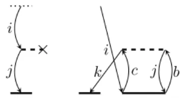
1.3. Diagrammatic techniques

A simple way to develop working equations is the usage of diagrams. Di- agrams are image representations of matrix elements, which provide a link to programmable expressions. The task of finding all necessary expressions is then replaced by finding all unique diagrams. Two example diagrams are shown in Fig. (1.1). The first diagram is connected to the bare excitation op- erator of the

side drawn as a small dashed horizontal line. Diagrams closed like this refer to matrix elements obtained by projections on covariant CSFs.

Open diagrams like the second one, on the other hand, refer to projections on

×

i j

i

k c j b

Figure 1.1.: Exemplary diagrams contravariant CSFs.

Bold dashed horizontal lines, or interaction lines, represent fragments of the Hamilton operator like the Fock operator

(first diagram) or the fluctuation potential

(second diagram). They have as many vertices as electrons they act on. Since the Fock operator is an one-electron operator the second vertex is crossed out. Non-dashed horizontal lines, representing the cluster operators

usually have an incoming and outgoing vertical line, which reflect the action of the operator on an electron. However, operators that remove (add) one electron from (to) a molecular system, as it is the case for cluster operators of ionized (electron attached) states, have one excess incoming (outgoing) line.

Vertical lines are orbital substitutions relative to the Fermi vacuum and labeled with orbital indices. They can point either downwards representing occupied orbitals (hole lines) or upwards for virtual orbitals (particle lines).

If vertical lines are connecting two vertices they are called internal. External lines have at least one open end. Exception from this rule are lines connected to the bare excitation operator: these lines are also considered external. With the following rules, diagrams can be translated into mathematical expressions:

•

Each closed loop containing exclusively internal lines contributes a factor of two.

•

The sign is given by (−1)

in which h is the number of hole lines and l the number of (closed plus non-closed) loops.

•

Summation over internal lines.

•

Horizontal lines contribute either an integral (bold dashed lines) or an

amplitude (non-dashed lines). The two-electron integrals take the form (out

in

in

), out labeled according to outgoing and in according to incoming vertical lines of a certain vertex 1 or 2. The Fock matrix is obtained similarly:

virtue of occupied (occ) and virtual (virt) indices rather than outgoing and incoming lines: t

1virt2...

. The bare excitation operators contribute nothing.

•

Vertical lines between bare excitation operators and interaction lines are dressed via similarity transformation with

amplitudes.

•

In local basis every particle line not connected to an integral gives rise to the PAO overlap matrix

.

For example, evaluation of the two diagrams in Fig. (1.1) with the given rules yields

−X

j

f ˆ

u

and

2

bcjk

(kc|jb)t

u

. (1.19)

Note that the left expression results from a diagram with a covariant CSF, the

right one from a diagram with a contravariant CSF.

cluster ionization potentials

The content of this chapter has been published already in Ref. [33]. Authors involved in this work were Dr. Denis Usvyat, Dr. Tatiana Korona and my supervisor Prof. Dr. Martin Schütz. This chapter is taken entirely from the above mentioned publication. Some minor changes and additional notes have been added.

2.1. Introduction

In section 1.1 the coupled cluster theory was briefly presented for treating molecules in their ground state. This chapter covers the formalism for excited states, in particular for ionized states. One very versatile approach is response theory [34]. From response functions frequency-dependent molecular proper- ties are obtained, from which expressions for the determination of excitation energies, transition strengths, polarizability, hyperpolarizabilities, etc. can be derived. This theory is used in the following to develop a formalism for ionized states and their ionization energies.

Another approach to excited (including ionized and electron attached) states is the equation-of-motion (EOM) CC framework. Methods for the calculation of ionization potentials (IPs) and properties of ionized states have been pre- sented before in the EOM-CC framework [35–45], yet to the author’s knowledge so far only for non-local canonical or natural orbitals, and without a DF based factorization of the Jacobian transforms. Note that ionization potentials can

15

also be simulated with existing programs for excitation energies by adding a very diffuse orbital to the space of virtual orbitals [39]. However, calculations employing this technique do not benefit from the lower scaling of a separate IP program.

2.2. Response theory for ionized states

As the time-dependent perturbation a formal non-physical operator is intro- duced, which destroys and creates a particle,

V(t) =

n

X

k=−n

exp(−iω

t)V(ω

), (2.1)

V(ω_k

) =

Y

(ω

)Y,

=

p

Y

(a

+ a

), (2.2)

with the perturbation strengths

(ω

) and the annihilation (a

) and cre-

ation (a

) operators in second quantization. By treating ionization and elec-

tron attachment processes together,

remains Hermitian. Together with the

symmetry properties ω

=

, and

(ω

) =

(ω

) the time-dependent

perturbation

is Hermitian. Since

is unphysical the “integrals” Y

of

operator

are set to one, for simplicity. With operator

exact linear response function for such a perturbation can then be written as

Y

=

I¯

h0|X|

Iih ¯ I|Y ¯

ω

(E

E

)

Iih ¯ I|X|0i ¯ ω + (E

E

)

+

A¯

h0|X|

Aih ¯ A|Y ¯

ω

(E

E

)

Aih ¯ A|X|0i ¯ ω + (E

E

)

=

pq

( X

I¯

h0|a^†_pβ|

Iih ¯ I|a ¯

ω

ω

−h0|a^†_pβ|

Iih ¯ I|a ¯

ω + ω

!

+

A¯

h0|a_pβ|

Aih ¯ A|a ¯

ω

ω

−h0|a_pβ|

Aih ¯ A|a ¯

ω + ω

!)

=

ij

X

I¯

h0|a^†_iβ|

Iih ¯ I|a ¯

ω

ω

− h0|a^†_iβ|

Iih ¯ I ¯

ω + ω

!

+

ab

X

A¯

h0|a_aβ|

Aih ¯ A|a ¯

ω

ω

− h0|a_aβ|

Aih ¯ A|a ¯

ω + ω

!

, (2.3)

where

Ii ¯ are the ionized eigenstates living in the Fock subspace F (M, N

1) with related energies E

, and

Ai ¯ the electron attached states with related energies E

living in F (M, N + 1). M and N denote the number of spin orbitals and the number of electrons of the system, respectively. The linear response function

Y

has poles for ionization energies ω

and electron affinities ω

. In this chapter only the first part of

Y

, containing the poles for ω

, is discussed. It contains only state functions for ground and ionized states. Ionized states are generated from ground state functions by an operator with one excess annihilator (cf. Eq. (2.8)). The time-dependent CC wavefunction after isolation of the phase can be written as

|

CCi

= exp(T

+

(t) + . . . )|0i, (2.4)

with

T⁽⁰⁾

=

+

+ . . . ,

(t) =

2

(t) +

(t) + . . . , (2.5) and

T⁽⁰⁾₁

= t

τ

= t

τ

,

= t

2

τ

= 1 2 t

τ

,

2

(t) = t

12

(t)τ

2

= t

(t)τ

,

2

(t) = t

2

(t)τ

2

= t

(t)τ

. (2.6) Note that Einstein convention is used above and in the following, i.e., repeated indices are implicitly summed up. Summations are written explicitly only if it is helpful for clarity.

In Eqs. (2.5) and (2.6) the particle rank m of related operators is introduced, i.e., the number of elementary operators of an operator string divided by two, as subscript indices in the individual

operators. For CC2 and CCSD the particle rank is truncated at m = 2 in the cluster operator. Furthermore, by virtue of the 2n + 1 rule it is sufficient to consider amplitudes up to first order with respect to

by superscripted numbers in parenthesis. Note that zeroth-order amplitudes with half-integer particle rank, as well as first order amplitudes with integer particle rank, are all zero.

The operators τ

in Eq. (2.6) are all spin-adapted:

τ

= a

a

+ a

a

, τ

= τ

τ

, (2.7)

τ

= a

, τ

= τ

τ

, τ

= τ

τ

. (2.8)

The operators in Eq. (2.7) with integer particle rank are spin- and particle-

conserving or singlet-coupled excitation operators, generating a singlet state

when being applied to the closed shell reference determinant

hand, the operators in Eq. (2.8) with half-integer rank produce a doublet state with S = M

=

and reduce the number of particles by one. As a sidenote, the LMO pair list for zeroth-order amplitudes t

is triangular, while it is not for the first-order amplitudes t

.

The contravariant

functions forming a biorthonormal set with the

functions take the form

h˜

µ

=

Φ ˜

= 1

2

)

,

µ

=

Φ ˜

= 1

6

+ τ

)

,

µ

2|

=

Φ ˜

=

)

,

µ

2|

=

Φ ˜

= 1

3

+ τ

)

. (2.9) With these information the time-averaged second-order quasienergy Lagrangian can be set up:

{²ⁿ⁺¹

L

(t)}

=

n

X

k=−n

hD

0

hV(−ω_k

),

(ω

)

CC

+ λ

D

˜ µ

h

V(−ωk

),

(ω

) +

(ω

)

CC

E

−

λ

m

(−ω

)ω

t

l

(ω

)

µ

CCi (2.10) +λ

(−ω

)

˜ µ

V(ω_k

) +

H⁽⁰⁾

,

(ω

) +

(ω

)

CC

where

= exp(T

)|0i is the unperturbed CC wavefunction,

µ ˜

=

µ

exp(−T

),

T⁽¹⁾_m

(ω

) = t

m

(ω

)τ

, with t

(t) =

n

X

k=−n

t

(ω

) exp(−iω

t), (2.11)

λ

(ω

) is defined analogously, and

is the unperturbed Hamiltonian. In

Eq. (2.10) the particle-rank index m runs over m = 1, 2 for zeroth-order multi- pliers λ

, and over m =

,

for first-order multipliers λ

(ω

) and amplitudes t

(ω

). The Lagrangian contains no products of

(ω

) cluster operators, since related diagrams cannot be closed, neither by operators with integer par- ticle rank nor in combination with one operator with half-integer particle rank.

This implies that the second derivative of

L

(t)}

with respect to the first-order amplitudes is zero, which is a substantial simplification relative to CC response theory for electronically excited states. The linear response func- tion with poles for the ionization potentials is obtained as the second derivative of

L

(t)}

with respect to the perturbation strengths :

hhX;

Y

= d

L

(t)}

d

(−ω)d

(ω) = η

t

+ η

t

, (2.12) with

η

l

= ∂

L

(t)}

∂

(−ω)∂t

(ω)

=

0

h

Y, τ_µ1

2

i

0

δ

2

+ λ

˜ µ

h

Y, τ³

2

i

0

δ

2

, (2.13) and m being integer and l half-integer. Note that in the first two summands of Eq. (2.10) only the reference

of the

remains since

cannot connect multiple

t

is obtained from the stationary conditions

(A

ωM)t

+ ξ

= 0, (2.14) with the CC Jacobian

A

ωM

= ∂

L

(t)}

∂λ

(−ω)∂t

(ω) , A

=

˜ µ

H⁽⁰⁾

, τ

CC

, (2.15)

metric

M

=

µ

(2.16) and

ξ

=

L

(t)}

∂λ

(−ω)∂

(ω) =

µ ˜

CCi =

µ ˜

0i , (2.17) with m and l both half-integer indices. From Eq. (2.17) it is clear that ξ

is non-zero for m =

. Therefore, t

has poles for the singular matrix

ωM (cf. Eq.(2.14)), which, in turn, leads to poles for these ω in the linear response function

Y

according to Eq. (2.12). The eigenvalues of the CC Jacobian

hence correspond to the ionization potentials of the molecular system as described by the CC model.

2.3. Approximate coupled cluster model CC2

As outlined earlier, CCSD scales as

. The motivation for CC2 is to obtain a cheaper coupled cluster method which still contains correlation energy unlike CCS. Christiansen et al. [9] presented this method 1995. CC2 is designed such that the ground state energy is correct through second order, in contrast to CCSD which is correct through third order. Therefore, the total energy is of MP2 quality, however, CC2 allows for calculating excitation energies and tran- sition moments. The CC2 model is based on the Møller-Plesset partitioning of the Hamiltonian,

H⁽⁰⁾

=

+

, (2.18)

with

representing the Fock operator, and

the fluctuation poten-

tial. The order with respect to the fluctuation potential, and with respect

to

is indicated by superscript numbers in brackets, and parenthesis, re-

spectively. In the following these superscripts are dropped for the Hamiltonian

and its fragments. Lower scaling and an energy correct through second order is

achieved by approximation of the CCSD amplitude equations: the singles am-

plitude equations remain unchanged and the doubles amplitude equations are

approximated to be correct through first order with respect to the fluctuation

potential,

0 =

˜ µ

H

ˆ +

H,

ˆ

0

, (2.19)

0 =

˜ µ

H

ˆ +

F,T⁽⁰⁾₂ i

0

, (2.20)

with the similarity-transformed Hamiltonian

H

ˆ = exp(−T

)H exp(T

). (2.21) The singles amplitudes have a special role: although singles amplitudes appear at second order with respect to the fluctuation potential for the first time, this is due to the fact that Hartree-Fock is used as a reference [11]. Otherwise, singles already appear at zeroth order. Since singles are important to approx- imate orbital relaxation effects they are assigned to be zeroth-order in

The similarity transformation of the Hamiltonian is a convenient way to keep the singles amplitudes in the equations. This transformation leads to dressed integrals,

(pq ˆ

λ

λ

λ

, (2.22) decorated with a hat. The coefficient matrices λ

and λ

transform from AO basis (indexed by Greek letters µ, ν, . . . ) to MO basis. They are calculated from the LMO and PAO coefficient matrices

and

overlap matrix

and zeroth-order singles amplitudes t

:

λ

= P

L

t

S

, λ

= L

λ

= P

, λ

= L

+ P

t

. (2.23)

These coefficient matrices are the origin for the fifth diagrammatic rule in

Sec. 1.3, stating that only vertical lines between the bra side and an interac-

tion line are similarity transformed. Looking closely at the four transformation

matrices reveals that only outgoing lines which point upwards (λ

) and in-

coming lines which point downwards (λ

) include the singles amplitudes. The

only possibility for such lines are vertical lines connecting the bra side with an interaction line. Vertical lines going out (λ

) or coming in (λ

) from below of an interaction line are not dressed.

The density fitting approximation can still be applied in a straightforward way,

(pq ˆ

(pq ˆ

)ˆ c

. (2.24) As a result, the three-indexed quantities are similarity transformed. The dressed Fock matrix is defined as

f ˆ

= ˆ h

+

i

2(ii ˆ

(iq ˆ

. (2.25)

In this work, constraints according to the local ansatz presented in Sec. 2.4.4 are imposed on the zeroth-order doubles amplitudes

:

T⁽⁰⁾₂

= 1 2

X

ij∈P₀

X

ab∈[ij]

t

τ

, (2.26)

with P

refering to the (restricted) ground state pair list. The pair list and domains for the ground state are determined on basis of spatial locality ar- guments. Detailed information for the test calculations can be found in Sec- tion 2.5.

The CC2 Jacobian for ionized states is obtained by differentiation of the time-averaged second-order quasienergy Lagrangian for the CC2 model, yield- ing

A

=

2 1

2 A¹

2 3 2

A³

2 1

2 A³

2 3 2

!

=



 D

˜ µ

2

hH, τ

ˆ

i

exp(T

)

0

E D

˜ µ

2

hH, τ

ˆ

i

0

E D

˜ µ

2

hW, τ

ˆ

2

i

0

˜ µ

2

h

F, τ_ν3

2

i

0





(2.27)

The ionization potentials ω

for the lowest ionized states

I ¯

are obtained by

solving the right eigenvalue problem

AR( ¯

I) = ω

I ). (2.28) To this end a Davidson procedure generalized to nonsymmetric matrices is employed [46, 47] such that only matrix trial-vector products

rather than the full matrix

I ¯

N

denotes a particular ionized state. N

is equal to the number of states treated in a multistate calculation. On the other hand, I

corresponds to a certain basis vector of the Davidson subspace, which, in turn, belongs to a certain I. At the start of every calculation and at a refresh of the subspace ¯ N

= N

. With every iteration basis vectors are added to the Davidson subspace and N

grows accordingly. No state-specific local approximations are introduced on the trial vectors U (I ) and eigenvectors R( ¯ I) at the CC2 level. Only the truncation of the zeroth-order doubles amplitudes is utilized in the computation of the intermediate V

(cf. Eq. (2.31)). Moreover, the locality in the orbitals is exploited for prescreening in the evaluation of the diagrams given below.

Diagrams for the CC2 Jacobian are shown in Fig. (2.1). From these the ex- pressions for the right matrix trial-vector product

(I ) are obtained.

The final working equations, including the factorization of ERIs according to the DF approximation, are

vⁱ

=

f ˆ

+ u

Z

+ ˆ f

u ˜

W

(ki ˆ

), (2.29)

= ˆ c

B ˆ

+ f

u

S

u

f

S

u

f

, (2.30) with the intermediates

Z

=

)V

, V

= ˜ t

c

fc

W

= c

u ˜

, B ˆ

=

(ki ˆ

). (2.31)

Amplitudes and trial vectors decorated with a tilde correspond to contravariant

× × ×

× ×

× × × ×

Figure 2.1.: Covariant diagrams of the CC2 Jacobian arranged in corresponding block structure and in order according to Eqs. (2.29) and (2.30). To each summand of these equations belong two consecutive diagrams, except the first one of

2 1

2

. Using contravariant

CSFs cancels the second diagram of each couple of diagrams in

2 1

2

and

2 3 2

.

bra

functions as defined in Eq. (2.9). They are calculated according to

˜ t

= 2t

t

, and u ˜

= 2u

u

. (2.32) For a clearer formulation the explicit dependence of trial vectors U and pro- ducts

on the ionized states is dropped.

As is evident from Fig. (2.1) fifteen covariant diagrams contribute to the CC2 Jacobian. However, only eight summands remain in the final working equations (2.29) and (2.30). This is an effect of the contravariant

CSFs and their corresponding contravariant amplitudes and trial vectors (Eq. (2.32)), as well as their ability to reduce the number of actual expressions in the working equations.

As a sidenote, the right matrix trial-vector produt

for the ADC(2), also known as TD-UCC[2]-H [8], Jacobian

is very similar to Eqs. (2.29)-(2.31).

Only the

part differs, reading instead

=

f

+ 1

2 u

(Z

+ Z

)

W

(ki|P ) (2.33)

and all integrals and Fock matrix elements are undressed. Since ADC(2) relies

on a MP2 ground state calculation the singles amplitudes t

are zero and hence ADC(2) is Hermitian.

2.4. Additional higher order diagrams

The CC2 model for ionized states as specified in Sec. 2.3 does by itself not provide ionization potentials of satisfactory accuracy. It is, however, used to generate initial guesses for the right eigenvectors R( ¯ I), as well as initial state-specific local approximations. Due to the generation of an electron hole through the ionization process, orbital relaxation effects are expected to be of greater importance for ionization potentials than for electronic excitation energies, where the CC2 model already provides acceptable accuracy for many applications.

In order to improve on the CC2 model, higher-order diagrams are added to the CC2 Jacobian, while still sticking to the m =

excitation space.

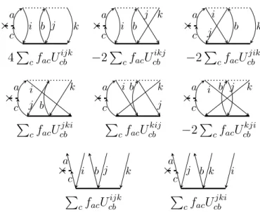
From Eq. (2.27) it is clear that the

2 1

2

and

2 3

2

submatrices are already complete in the sense that they contain all possible diagrams, whereas for the submatrices

2 1

2

and

2 3

2

this is not the case. The latter are only correct

to first- and zeroth-order with respect to the fluctuation potential

tively. Therefore, the order of these submatrices is increased step by step. For

further reference the methods of this hierarchy are called IP-CCSD[k]

, with

k

[0, 1, 2, f]. This acronym implies that

used in the eigenvalue problem

(2.28) is an approximation to the CCSD Jacobian, correct to order k with re-

spect to

on top of a CC2 ground state calculation. Consequently, the pure

CC2 approach corresponds to the acronym IP-CCSD[0]

. IP-CCSD[f]

as

well as IP-CCSD

denote the full CCSD Jacobian.