Dissertation submitted to the
Combined Faculties for the Natural Sciences and for Mathematics of the Ruperto-Carola University of Heidelberg, Germany
for the degree of Doctor of Natural Sciences
presented by Diplom-Physicist: Uwe Langend¨orfer
born in: Karlsruhe
Oral examination: 18th July, 2001
Oxygen isotopes as a tracer of biospheric CO 2 gross fluxes
- a local feasibility study -
Referees: Priv.-Doz. Dr. Ingeborg Levin Prof. Dr. Konrad Mauersberger
Abstract
Oxygen isotopes as a tracer of biospheric CO2 gross fluxes - a local feasibility study -
Quantitative knowledge of gross biospheric CO2 fluxes is crucial in atmospheric carbon cycle budgeting, especially in view of unknown biospheric feedback mechanisms to an increasing atmospheric CO2 mixing ratio or to temperature changes. The18O/16O ratio of CO2 has the potential to separate respiration and assimilation fluxes because of their characteristic iso- topic signatures derived from equilibration with respective water reservoirs (i.e. soil and leaf water). The associated processes were investigated here on a local scale during three intensive measurement campaigns in a natural boreal forest reserve in Russia. Diurnal cycles of atmo- spheric CO2 and its stable isotope ratios, of the18O/16O ratio of atmospheric water vapour, leaf and soil water were measured. The data sets were then quantitatively interpreted in a
222Radon-transport-calibrated 1-D canopy box model. On the basis of observations and plant physiological parameterisations, for the first time, the feasibility to separate gross ecosystem CO2 fluxes could be demonstrated. Reasonable agreement with classical local scale methods could be achieved, whereby the model results are most sensitive to the parameterisation of leaf internal CO2 gradients. Concurrent year-round aircraft CO2 and stable isotope obser- vations showed that the biospheric ecosystem 18O signals are effectively transferred into the free troposphere. Provided that adequate parameterisations on the leaf scale can be achieved, this gives the perspective to successfully use the 18O/16O ratio in atmospheric CO2 within coupled mesoscale or even global biosphere-atmosphere models of the carbon cycle.
Zusammenfassung
Sauerstoffisotope als Indikator f¨ur biosph¨arische CO2 Bruttofl¨usse - eine lokale Machbarkeitsstudie -
Die Bestimmung der biosph¨arischen Brutto-CO2-Fl¨usse ist notwendig zur quantitativen Bi- lanzierung des atmosph¨arischen CO2-Mischungsverh¨altnisses, insbesondere im Hinblick auf m¨ogliche biosph¨arische R¨uckkopplungen auf den globalen atmosph¨arischen CO2-Anstieg oder auch Klimaver¨anderungen. Das18O/16O-Verh¨altnis im atmosph¨arischen CO2 erlaubt es po- tentiell, die Assimilations-und Respirationsfl¨usse zu separieren, aufgrund ihrer charakteristis- chen Isotopensignaturen, welche durch ¨Aqulilibrierungsprozesse mit den zugeh¨origen Wasser- reservoiren (Blatt-und Bodenwasser) zustande kommen. Im Rahmen dieser Arbeit wur- den diese Prozesse w¨ahrend dreier intensiver Feldkampagnen in einem nat¨urlichen borealen Wald in Rußland untersucht. Es wurden Tagesg¨ange von CO2 und seinen stabilen Isotopen- verh¨altnissen, der 18O-Isotopie des Luftwasserdampfs sowie des Blatt- und Bodenwassers gemessen. Die Messungen wurden mit Hilfe eines eindimensionalen, mit222Radon transport- kalibrierten, ¨Okosystemmodells untersucht. Auf der Basis der Messungen und mit Hilfe von pflanzenphysiologischen Parametern konnte zum ersten Mal gezeigt werden, daß es m¨oglich ist, die CO2- ¨Okosystembruttofl¨usse zu separieren. Das Modell liefert Ergebnisse, die sich gut mit klassischen lokalen Methoden vergleichen, es zeigt jedoch eine starke Abh¨angigkeit der Fl¨usse von der Parameterisierung des blattinternen CO2-Gradienten. Parallele, quasi- kontinuierliche Flugzeugmessungen von CO2und seinen stabilen Isotopenverh¨altnissen zeigen dar¨uber hinaus, daß sich die kleinskaligen biosph¨arischen 18O-Signale in der freien Tro- posph¨are abbilden. Dies er¨offnet die M¨oglichkeit, das 18O/16O-Verh¨altnis im CO2 in gekop- pelten mesoskaligen oder sogar globalen Biosph¨are-Atmosph¨are-Modellen zu nutzen, wenn eine ad¨aquate Parameterisierung auf der Blattebene gefunden werden kann.
Contents
1 Introduction 3
1.1 The Global Carbon Budget . . . 4
1.2 Temporal and Spatial Evolution of CO2 in the Atmosphere . . . 6
1.2.1 CO2 Mixing Ratio . . . 6
1.2.2 13C/12C Isotope Ratio of CO2 . . . 9
1.2.3 18O/16O Isotope Ratio of CO2 . . . 13
1.3 Summary . . . 16
2 Terrestrial Biospheric CO2 Exchange 18 2.1 CO2 Mixing Ratio . . . 18
2.1.1 Assimilation . . . 21
2.1.2 Respiration . . . 22
2.1.3 Boundary Layer and Canopy Meteorology . . . 23
2.2 CO2 Isotope Ratios . . . 26
2.2.1 13C/12C . . . 26
2.2.2 18O/16O . . . 28
2.3 Open Questions and Motivation for this Work . . . 32
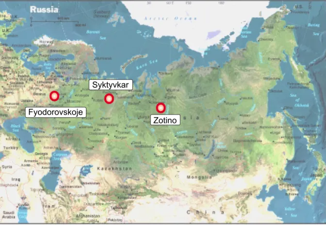
3 Experimental 33 3.1 The Areas of Investigation . . . 33
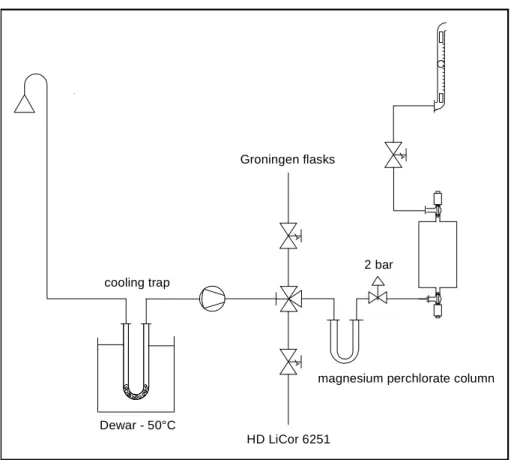
3.2 Measurements . . . 35
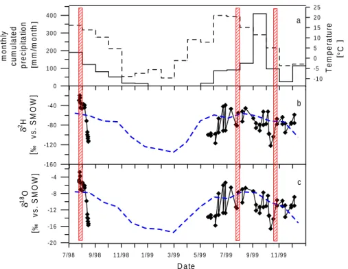
4 Results of the Field Campaigns in Russia 39 4.1 Hydrological Characterisation . . . 39
4.2 Summer 1998 . . . 40
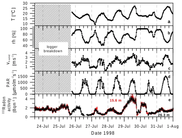
4.2.1 Meteorology . . . 40
4.2.2 CO2 Mixing Ratio and Stable Isotopes . . . 42
4.2.3 H162 O/H182 O of Plant Tissue . . . 47
4.3 Summer 1999 . . . 49
4.3.1 Meteorology . . . 49
4.3.2 CO2 Mixing Ratio and Stable Isotopes . . . 50
4.3.3 H162 O/H182 O of Plant Tissue and Water Vapour . . . 53
4.4 Autumn 1999 . . . 55
4.4.1 Meteorology . . . 55
4.4.2 CO2 Mixing Ratio and Stable Isotopes . . . 55
4.4.3 H162 O/H182 O of Plant Tissue and Water Vapour . . . 58
4.5 Summary of Experimental Findings and Conclusion . . . 60 1
5 1-D 222Radon Calibrated Canopy Model 62
5.1 Model Set- up . . . 62
5.2 Turbulent Vertical Transport . . . 62
5.3 Parameterisation . . . 64
5.4 Results . . . 67
5.4.1 Standard Simulation . . . 67
5.4.2 Sensitivity Runs . . . 72
5.5 Discussion & Prospects . . . 81
6 Regular Flights at Syktyvkar 83 6.1 Seasonality . . . 83
6.2 Longitudinal Variation over Euro-Siberia . . . 85
Outlook 89
A Model code 9 0
List of Figures 106
List of Tables 110
Bibliography 111
Acknowledgements 120
Chapter 1
Introduction
”As early as at the beginning of this century, the great french physicists Fourier and Pouillet had established a theory according to which the atmosphere acts extremely favourably for raising the temperature of the earth’s surface. They suggested that the atmosphere functioned like the glass in the frame of a hotbed.”...”The main components of the air, oxygen and nitrogen, do not absorb heat to any appreciable extent, however the opposite is true to a high degree for the aqueous vapour and carbonic acid in the air although they are present in very small quantities. And these substances have the peculiarity that to a great extent they absorb the heat radiated by the earth’s surface while they have little effect on the incoming heat from the sun.
If now the quantity of carbonic acid in the air is increased, the temperature of the earth’s surface increases.” 1
Svante Arrhenius principal predictions on the increase of the earth’s surface tempera- ture linked to the simultaneous increase of carbon dioxide (the atmospheric precursor of carbonic acid mentioned by Arrhenius) still hold true after the modern scientific perceptions achieved in the last hundred years. He was the first to quantify the potential temperature changes due to an increasing CO2 concentration in the atmosphere, which again was explained by a colleague of Arrhenius, Arvid H¨ogbom (1857-1940), to originate from anthropogenic coal burning. While calculating this so called ”green house effect” he also recovered a relevant accompanying feedback process, namely the increases of atmospheric water vapour: ”This also causes some increase in the amount of aqueous vapour in the air, resulting in a slight intensification of the effect.”1 Therefore, he indirectly stated the present day finding that atmospheric interactions and variabilities behave highly non-linearly.
Besides the other major greenhouse gases methane, nitrous oxide and the halocarbons, carbon dioxide provides the largest individual contribution of 1.46 Wm−2 (about 60 %) to the overall radiative forcing due to changes from pre-industrial to present day conditions [IPCC, 2001]. Therefore, the understanding of the carbon cycling processes and the pre- dictability of the atmospheric CO2 concentration development -under prescribed emission scenarios -are framing the potential of political decision making with the intention to stabilize future atmospheric CO2 concentration.
As Arrhenius and H¨ogbom were formulating their scientific interest with the focus on long time scales, mainly directed towards exploring the extension and effects of the last glaciation, present-day scientific questions are asked within the context of the public, and more and more political “global change” debate:
1Excerpts of notes from a lecture ”Nature’s heat storage” given by Prof. Svante Arrhenius (1859-1927) at Stockholm University on third of February 1896 (printed in Swedish in Nordisk Tidskrift 14(1896), 121-1130).
3
• How will the atmospheric CO2 concentration develop due to future anthropogenic CO2 emissions ?
• What are the key feed back reactions of the oceanic and the terrestrial carbon systems on changes of the climate system ?
1.1 The Global Carbon Budget
The prerequisite to predict the future evolution of the CO2 concentration in the atmosphere, and therewith the potential global climate impact of future elevated CO2 in the atmosphere, is understanding of processes that control the actual carbon system. The present quantitative knowledge of the net fluxes between the three major carbon reservoirs, the atmosphere, the oceans and the terrestrial biosphere, is summarized in Table 1.1. Fluxes are given in PgC yr−1 2. The determination of the annual net fluxes is a general (measurement) problem, if Table 1.1:Global atmospheric carbon balance based on CO2 and O2 budgets [Heimann, 2000]
(fluxes in PgC yr−1).
1980 to 1989 1990 to 1999
Atmospheric increase 3.3±0.1 3.2±0.1
Emissions(fossil fuel, cement) 5.4±0.3 6.3±0.4
Ocean-atmosphere flux -2.0±0.6 -1.8±0.6
Land-atmosphere flux* -0.2±0.7 -1.4±0.7
*Partitioned during 1980 to 1989 as follows (range of uncertainty given in parenthesis):
Land-use change 1.6 (0.5 to 2.4)
Residual terrestrial sink -1.8 (-3.7 to 0.4)
one bears in mind the numbers of the annual gross fluxes between the reservoirs given in Table 1.2. Here small differences, the net fluxes, between large numbers, the gross fluxes, are particularly hard to determine precisely as the net fluxes are about two orders of magnitude smaller than the ’one-way’ gross fluxes. The gross fluxes given in Table 1.2 represent mean Table 1.2: Gross fluxes (PgC yr−1) between the reservoirs and inventory (PgC) of the reser- voirs within the global carbon cycle over the period 1980 to 1989 [Houghton et al., 1996].
Carbon reservoir Content Gross flux Gross flux to atmosphere from atmosphere (PgC) (PgC yr−1) (PgC yr−1)
Ocean 39000 90 -92
Land biosphere 2200 60 -61.4
Atmosphere 750 --
values, and are itself afflicted with uncertainties in the order of 30 % for the lands biosphere
21 Pg = 1015g = 1 Gigaton
1.1. THE GLOBAL CARBON BUDGET 5
and of about 15 % for the ocean fluxes. Furthermore, the uncertainties of the fluxes between the reservoirs given in Tables 1.1 and 1.2 illustrate another principal problem of balancing the global carbon cycle: the possible scientific accessibility of each reservoir and flux, respectively.
The most precise value of the determined inventories within the global carbon cycle is the change of the atmospheric CO2 inventory with an uncertainty of about ±4 %. This is due to the fact, that the atmosphere is a relatively well mixed system. Furthermore the atmo- sphere is accessible easily by measurements, which is done worldwide [Francey et al., 1990;
Levin et al., 1995; Nakazawa et al., 1997]. The largest monitoring network is operated by NOAA/CMDL (National Oceanic & Atmospheric Administration / Climate Monitoring &
Diagnostics Laboratory) since 1967 with stations shown in Figure 1.1 [Conway et al., 1994].
The first station that started long term observation of CO2 mixing ratios was initiated in the middle of the Pacific ocean at Mauna Loa, Hawaii, by C.D. Keeling in 1958 [Keeling, 1958].
Figure 1.1: The NOAA/CMDL monitoring station network [Pieter Tans, NOAA, http://www.cmdl.noaa.gov]
According to Table 1.1 the emission flux of anthropogenic carbon is the second best known value in the budget with an uncertainty of about 7 %. These data are derived from global fossil fuel burning and cement production emission statistics including the information of the spatial distribution of the emissions [Marland and Boden, 1997]. The observed rise in atmospheric CO2 amounts to only about 50 to 60 % of the anthropogenic emissions, which implies that the residual carbon has to be stored in the oceans and/or the terrestrial biosphere. Whereas the net ocean-atmosphere flux (via uptake of CO2 through air-sea exchange) can be determined as an atmospheric sink with a circa 30 % accuracy, the land-atmosphere fluxes (via the gross fluxes resulting from photosynthesis as an atmospheric sink and ecosystem respiration as an atmospheric source) net direction from 1980 to 1989 can not even unequivocally be stated.
For the period from 1990 to 1999, however, a significant net sink flux from the atmosphere to the land biosphere could be detected. The principal problem in determining the fluxes between the land biosphere and the atmosphere is twofold: First, the net flux has to be separated into two components as shown in Table 1.1. Changes in land use cause a net source for atmospheric CO2 due to deforestation, a process that is believed to be counterparted by a residual terrestrial CO2 sink. The second principal problem is caused by the heterogeneity of the terrestrial biosphere itself. The global biosphere consists of a large number of different ecosystems that may also variably react on climatic conditions. Furthermore, it is well known, that the biospheric exchange does not only act on a daily or seasonal timescale but also on a long term scale, a fact that complicates future predictions. As the net CO2 emission flux of land use change is determined with an accuracy of only about 50 %, the error of the estimated residual terrestrial sink is about 100 %. For this reason, the accurate quantification of regional biospheric surface fluxes of CO2 is essential to minimize the lack of information on larger scales by (model) extrapolation up to the global scale.
1.2 Temporal and Spatial Evolution of CO
2in the Atmosphere
1.2.1 CO2 Mixing Ratio
Besides the investigation of the actual processes that control the exchange of carbon between the respective pools, the past status of the atmosphere and the global climate yield basic information to explore the global climate system. The inspection of the anthropogenically undisturbed system should provide the natural amplitudes of the relevant climate signals.
Therefore, the significance of the recent changes including the anthropogenic influence can largely benefit from the assessment of past variations.
Although the degree and chronology of change observed in climate archives may differ from actual and future variations, they provide an important insight into the system. The most valuable perception is the strong association between CO2 and temperature changes during glacial-interglacial transitions gained from ice core measurements. Figure 1.2 presents the early results of the Vostok ice core, drilled in Antarctica [Jouzelet al., 1993].
After the recent extension of this ice core back to the past 420,000 years, four glacial- interglacial cycles are covered by this record. The main result of these extensive studies are [Jouzel et al., 1993; Petitet al., 1999]:
• The present-day high atmospheric load of the two major greenhouse gases, CO2 and CH4, seems to be unique and has never been observed in the last 420,000 years. CO2 mixing ratios in the atmosphere varied between 180 to 200 ppm3during glacial and 280 to 300 ppm during warm periods. These values are to be compared with recent annual mean atmospheric CO2 mixing ratios in Antarctica of about 368.2 ppm; ∼21 % more than the highest values detected in the Vostok core (on the basis of latest data at the Neumayer station, Antarctica, with an annual mean CO2 mixing ratio of 365.22 ppm [Schmidt et al., 2001], assuming a CO2 growth rate of about 1.5 ppm per year for 2000 and 2001).
• There is a strong correlation between the changes in temperature4 and the greenhouse gases; the succession of the changes through the climate periods was similar.
31 ppm = 1 part per million, mol fraction
4The temperature anomalies relative to the present temperature are derived fromδD (H2O)ice variations [Petitet al., 1999].
1.2. TEMPORAL AND SPATIAL EVOLUTION OF CO2 IN THE ATMOSPHERE 7
2 0 0 2 4 0 2 8 0 3 2 0
CO2 [ppm]
0 1 0 0 0 0 0 2 0 0 0 0 0 3 0 0 0 0 0 4 0 0 0 0 0
A g e (y e a rs B P ) -1 2
-8 -4 0 4
Temperature change [ °C]
Figure 1.2:The Vostok (Antarctica) ice core record over the past 420,000 years [Jouzel et al., 1993; Petit et al., 1999]. Top: CO2 concentration, bottom: temperature anomalies relative to present temperature.
Still the remaining open question and matter of debate left from these studies is: What are the driving forces of natural climate changes? The Vostok ice core temperature, CO2 and CH4 increase more or less in phase during terminations [Petitet al., 1999]. The time, and therefore depth resolution of an ice core is restricted by the ubiquitous uncertainty in gas- age/ice-age differences. Petit et al., [1999] state this uncertainty to be well over ± 1 kyr.
For that reason, they could not detect any significant phase shift between the changes in temperature and the greenhouse gases. Any statements on a potential principle of cause and effect of climate changes are thus still impossible. However, in a recent study, Fischer et al.,[1999] investigated parts of the Vostok core and the Taylor Dome core (also Antarctica) around the last three glacial terminations in high time resolution. They found that CO2 mixing ratios increased by 80 to 100 ppm 600±400 yearsafter the warming of the last three deglaciations. CO2 concentrations were also observed to stay high for several thousands of years during glaciations. These results are based on an assumed gas-age/ice-age uncertainty of 100 to 1000 years [Fischeret al., 1999]. They could imply that temperature variations are driving the burden of greenhouse gases in the atmosphere due to their effect on the ocean- atmosphere carbon transfer (increasing with temperature), the control of land ice coverage and the build-up of the terrestrial biosphere. But the identification of a time lag between temperature and CO2 changes smaller than 1000 years of Fischer et al., [1999] takes the present knowledge of ice core signals to a limit and is therefore critizised [Stauferet al.,1993;
Petitet al., 1999].
Still the discussion on the uncertainty of gas-age/ice-age and the possible interpretation of ice core records is ongoing and the question of what is the hen and what is the egg in natural climate change remains unanswered. Especially the reaction of the global climate to the anthropogenic emissions of greenhouse gases since the industrialisation can not be evaluated. Therefore, the scientific focus is largely directed towards the interpretation of recent measurements performed worldwide (Figure 1.1).
CO2measurements at the Pacific Mauna Loa station since 1958 constitute the longest con- tinuous record of direct atmospheric CO2 concentrations available in the world. The Mauna Loa site is considered one of the most favorable locations for measuring undisturbed air because possible local influences of vegetation or human activities on atmospheric CO2 con- centrations are minimal and any influences from volcanic events can be excluded from the records. The Mauna Loa record (Figure 1.3) shows a 16.6 % increase in the mean annual mix- ing ratio, from 315.83 ppm of dry air in 1959 to 368.37 ppm in 1999 [Keeling and Whorf, 2000].
1 9 6 0 1 9 7 0 1 9 8 0 1 9 9 0 2 0 0 0
3 1 0 3 2 0 3 3 0 3 4 0 3 5 0 3 6 0 3 7 0
CO2[ppm]
B a rro w , 7 1 °N - 1 5 6 °W M a u n a L o a , 1 9 °N - 1 5 5 °W S o u th P o le , 8 9 °S - 2 4 °W
Figure 1.3: The SIO (Scripps Institution of Oceanography) atmospheric CO2 records from Barrow (Alaska), Mauna Loa (Hawaii) and the South Pole (Antarctica) [Keeling and Whorf, 2000].
Detailed analysis of the Mauna Loa record and the comparison with other time series at Barrow and at the South Pole delivers significant temporal and spatial differences of the CO2 concentration variabilities:
• There is a growing difference in annual mean CO2 concentration between the Northern and Southern Hemisphere ([CO2]M aunaLoa -[CO2]SouthP ole: changing from ∼0.5 ppm in 1958 to∼2.5 ppm in 1994). Furthermore, this difference is observed to scale linearly with fossil fuel CO2 emissions from 1959 to 1992 [Keelinget al.,1989; Heimann, 1999].
• The peak-to-peak amplitudes of the seasonal cycles are increasing northward from about 1 ppm at the South Pole to about 15 ppm in the boreal forest zone of the Northern Hemisphere (55 to 65 ◦N). This cycle is mainly caused by the seasonal uptake and re- lease of atmospheric CO2 by the terrestrial biosphere and to a small portion by oceanic processes [Heimann et al., 1989b; Keeling et al., 1995]. The amplitude is observed to increase with time (e.g. from 5.2 ppm from the beginning of the Mauna Loa record in 1958 to 5.8 ppm in the 1980s). As this increase is not well correlated with the CO2
1.2. TEMPORAL AND SPATIAL EVOLUTION OF CO2 IN THE ATMOSPHERE 9
concentration increase, a more or less significant evidence for CO2 fertilization of the terrestrial vegetation is discussed by several authors [Enting, 1987; Manning, 1993; Idso and Kimball, 1993; Heimannet al., 1996]. However, the changes in biological activity of the terrestrial biosphere can not necessarily be causally connected to increased pho- tosynthetic storage [Houghtonet al., 1996].
• The growth rate of 2.9 ppm yr−1 of the Mauna Loa record between 1997-98 rep- resents the largest single yearly jump since the Mauna Loa record began in 1958 [Keeling and Whorf, 2000]. Since 1975 the average increase is 1.5 ppm yr−1, with a minimum of 0.5 ppm yr−1 between 1991-92 and maximum growth rates of 2.0 ppm yr−1 from 1988-89. Because fossil fuel emissions after 1985 increased quite linearly at a rate of 0.1 to 0.2 PgC yr−1 [Bodenet al., 1994] the variability of the growth rate must be due to variations in the source/sink behaviour of the terrestrial biosphere and the ocean, respectively.
These findings demonstrate that there must be strong sink/source variabilities currently absorbing/respiring CO2 at the Earths surface, whereby both, the ocean and the terrestrial biosphere may contribute. As the budgeting of the global carbon cycle with the aid of at- mospheric CO2 concentration observation and ocean global circulation modelling is limited, further CO2 inert tracers are essential to distinguish between land-atmosphere and ocean- atmosphere fluxes.
1.2.2 13C/12C Isotope Ratio of CO2
The CO2 molecule consists of one carbon and two oxygen atoms. The element carbon is found to exist naturally as the stable isotopes12C and 13C and as a radioactive isotope 14C (half-life: 5730 years). Oxygen is an element that naturally exists as three stable isotopes
16O, 17O and18O. In the following considerations and the work presented here the focus will be on the processes in which the stable isotope ratios13C/12C and18O/16O are involved.
Isotopic ratios are usually reported in the standardδ-notation:
δErare=
Rsample
Rstandard −1
·1000 [o/oo] (1.1)
with e.g.
R=
[Erare] [Emain]
and
Rsample : isotopic ratio of the sample Rstandard : isotopic ratio of the standard
Emain : main isotope of the element “E” (e.g. 12C, 16O) Erare : rare isotope of the element “E” (e.g. 13C, 18O)
The reference standard is Vienna Pee Dee Belimnite (VPDB) (discussed in Allison et al.,[1995]), a virtual material related to the original Pee Dee Belimnite (PDB) [Craig, 1957].
The 13C/12C ratio of VPDB is taken from the PDB (13C/12C (PDB) = 1.1237 ×10⁻²).
The 18O/16O ratio is related to the isotopic ratio of Vienna Standard Mean Ocean Water (VSMOW) and the δ18O value of VPDB on the SMOW scale (18O/16O (SMOW) = 2.0088
×10−3, for details see Allison et al., [1995], Gonfiantini et al., [1995] and Neubert [1998]).
The reference materials are distributed by the International Atomic Energy Agency (IAEA) in Vienna.
A fractionation associated with a CO2flux from a reservoirAto a reservoirBis generally defined with a fractionation factorα as
αA→B = RA RB
(1.2) with e.g.
R=
13C
12C
Ifα >1, reservoirB is referred to as isotopically depleted with respect to reservoirA, and vice versa ifα <1, reservoirBis referred to as isotopically enriched. Furthermore, the fractionation is defined as
= (α−1)×1000 [o/oo]
Generally speaking, the 13C/12C isotope ratio in atmospheric CO2 gets modified during ex- change between CO2 reservoirs. Therefore, the isotope ratio of CO2 is a potential tracer of the global partitioning between the fluxes of atmospheric CO2 to the oceans and the land biosphere, respectively. This is due to the fact that plant CO2 uptake via photosynthesis strongly discriminates against 13C which causes the 13C/12C ratio of plant tissues to be smaller (also referred to as isotopically depleted) than the13C/12C ratio of atmospheric CO2. The repatriation of CO2 to the atmosphere via plant respiration is not observed to change the isotopic composition of CO2, CO2 from this source is, therefore, also depleted in13C. The degree of depletion is specific to the plant’s genome and varies from about=17 to 19o/oo for C3 plants to about 4 to 5o/oo for C4 plants [Vogel 1980; Farquhar et al., 1989]. Discrimination also depends on plant physiological parameters, which will be discussed in more detail in chapter 2.2.1. As the uptake of CO2 in the ocean is associated with a smaller depletion of only about =1o/oo [Mook, 1994] the isotopic signatures of the ocean-atmosphere CO2 flux and the land-atmosphere CO2 flux differ significantly.
The 13C signature of fossil fuel CO2 emissions is also depleted due to the biologi- cal origin of fossil energy sources. There is a dependence of the 13C signature on the type of fuel and its specific region of origin. The 13C/12C ratio of oil ranges from δ13C = -30o/oo to -26.4o/oo, natural gas carries a signature of about δ13C = -44o/oo, and coal of aboutδ13C = -24.1o/oo [Andres et al., 1999]. The global mean value of the 13C signature of fossil fuel CO2 is determined to -28.4o/ooin the period from 1990 to 1992 [Andreset al., 1993]
and changed to -29.4 ± 1.8o/oo in 1995 (personal communication with R. J. Andres in [Battleet al., 2000]). The shift in time to a lower 13C content coincides with a pro rata displacement from coal towards natural gas burning. This trend could directly be observed via atmospheric measurements on a regional scale in Heidelberg, Germany. Schmidt [1999]
found a change of the fossil CO2 δ13C source signature fromδ13C = -28.6±0.6o/ooin 1982/83 toδ13C = -38.5± 1o/oo in 1996.
As a consequence of the input of fossil fuel CO2 into the atmosphere, with a recent δ13C signature of -7.9o/oo, the13C content of atmospheric CO2 is decreasing with time. Figure 1.4 illustrates, that the decrease of the 13C/12C ratio of atmospheric CO2 is anticorrelated to the increase of the atmospheric CO2 concentration. The CO2 and δ13C data presented in Figure 1.4 are gained from ice core measurements (Law Dome, Antarctica), which could be chronologically linked to recent atmospheric measurements at Cape Grim, Antarctica.
The observed increase in the atmospheric CO2 mixing ratio from about 280 ppm to 350 ppm within the last 1000 years is accompanied with a decreasingδ13C signature from about -6.4o/oo to -7.8o/oo. The trend in the atmospheric13C signal is, however, also a function of the changing land use. As the global net storage of carbon in the biosphere translates directly in an isotopic enrichment of the atmospheric13C signal, a net source behaviour of the land’s
1.2. TEMPORAL AND SPATIAL EVOLUTION OF CO2 IN THE ATMOSPHERE 11
Figure 1.4:Law Dome (Antarctica) ice core CO2 record (a) [Etheridgeet al., 1996] andδ13C record (b) [Francey et al., 1999] (from [Trudinger et al., 1999]).
biosphere leads to an isotopic depletion of the atmospheric 13C signal. Since there is no, or only a negligible, fractionation occurring during the combustion and respiration of fossil, plant or soil carbon, both, industrial and land use changes cause similar changes in the atmospheric
13C signal.
Figure 1.5 illustrates the present global latitudinal distribution of the 13C/12C ratio of carbon dioxide in the marine boundary layer. The Northern Hemisphere CO2 is depleted in
13C with respect to the Southern Hemisphere CO2. The North Pole minus South Pole gradient in δ13C is about -0.3o/oo [Trolier et al., 1996]. This is interpreted as a direct consequence of the predominant emissions of fossil fuel CO2 in the Northern Hemisphere, which can also be manifested in the actual north-south gradient of CO2 mixing ratios of about 3 ppm (see also Figure 1.3). The correlated behaviour of CO2 and theδ13C signature is also observed in the differences of the amplitudes of the seasonal δ13C cycles between the hemispheres. The growing impact of biospheric activity, principally increasing from South to North, results in higher amplitudes in theδ13C (CO2) in northern latitudes.
There have been several global modelling studies which also include the 13C signature of atmospheric CO2 simulating the carbon exchange within the ocean-land-atmosphere system [i. e. Francey et al.,1995; Keeling et al.,1995; Ciais et al.,1995b]. In principal, these studies allow one to distinguish between ocean-atmosphere and land-atmosphere fluxes using the strongly different 13C fractionation factors mentioned above. The most recent study con- cludes, that there was a strong terrestrial biospheric sink in the mid 1990s in contrast to a more or less neutral biosphere in the 1980s [Battleet al., 2000]. Via an inverse modelling approach Ciais et al. [1995a] located a large terrestrial sink in the temperate latitudes of the Northern Hemisphere for the years 1992 and 1993, that reached roughly half of the mag-
Figure 1.5: 3-dimensional global latitudinal distribution of δ13C in atmospheric CO2 in the marine boundary layer. The surface represents data smoothed in space and latitude. [Jim White, NOAA, http://www.cmdl.noaa.gov]
nitude of fossil fuel emissions. Moreover these studies show a highly variable behaviour of the partitioning between ocean-atmosphere and land-atmosphere fluxes in space as well as in time. Whereas the total net flux in the latitudinal band from 30◦N to 90◦N from atmosphere to land and ocean was calculated to 4.6 PgCyr−1 in 1992, it decreased to 3.7 PgCyr−1 in 1993. Even more did the partitioning ratio of the fluxes atmosphere-land/atmosphere-ocean change for the same latitudinal band: from 13.1 in 1992 to 4.6 in 1993. [Ciais et al., 1995a].
The uncertainties of this approach illustrate the process dependency of the CO2 exchange and may also explain the high temporal variabilities via unknown feedback mechanisms. The process based uncertainties are principally threefold:
• The calculation of the discrimination of13C by plant photosynthesis in biosphere models is a function of the CO2partial pressure in the chloroplasts and other plant physiological parameters. The uncertainty of the13C discrimination is in the order ofδ=1o/oo, which contributes about 7 % to the uncertainty of the global atmosphere-land flux.
• The ‘isotopic disequilibrium’ of the soil CO2 flux: As the 13C content of atmospheric CO2is decreasing with time due to fossil fuel emissions, organic carbon in soils contained less depleted 13C in the past than today. Or in other words: carbon that is respired is isotopically enriched compared to carbon that is fixed photosynthetically at the same time. This is due to the time lag between carbon fixation via photosynthesis and the respiration of soil carbon because of the residence time (in the order of 30 to 100 years) of carbon in the biosphere (discussed by Ciaiset al., [1999]). This uncertainty is about 30 %, which contributes about 4 % to the uncertainty of the global atmosphere-land net
1.2. TEMPORAL AND SPATIAL EVOLUTION OF CO2 IN THE ATMOSPHERE 13
flux.
• The ‘isotopic disequilibrium’ of the ocean CO2flux, in principle the same mechanism as the soil disequilibrium, causes an uncertainty of about 30 %, which contributes about 25 % to the uncertainty of the global atmosphere-ocean flux.
These uncertainties illustrate the strong dependency of the models on an accurate knowledge of the controlling processes of carbon exchange between the atmosphere and the terrestrial biosphere and the oceans. Beyond that, however, the use of time series of13C/12C to determine a global CO2 budget is also seriously limited by the measurement precision of the atmospheric
13C/12C CO2 ratio and the density of the global monitoring network. At present, model calculations determine net source/sink fluxes with an uncertainty, which has the same order of magnitude as the fluxes themselves [Ciaiset al.,1995b; Ciais and Meijer, 1998]. Therefore, a strong effort is undertaken at present to intercompare the different monitoring networks and to reach the required measurement precision of 0.01o/oo forδ13C. Despite this, the status quo of the13C modelling approaches after all permits a reasonable detection of atmosphere- land-ocean fluxes on a regional scale.
1.2.3 18O/16O Isotope Ratio of CO2
In principle, the 18O/16O ratio of atmospheric CO2 gets modified in the same way as the
13C/12C ratio during CO2exchange processes between the respective carbon reservoirs. How- ever, the basic difference between the observed 13C/12C and 18O/16O ratios of atmospheric CO2 is due to the fact that gaseous CO2 may exchange an 18O atom with water according to the isotopic equilibrium reaction:
H218O(l)+C16O16O ↔H++ [HC16O16O18O]−(aq)↔H216O(l)+C16O18O(g) (1.3) The equilibrium fractionation,eq−CO2, between the oxygen in water and CO2 is dependent on temperature according to:
eq−CO2(T) = 17604/T−17.93 (1.4) with T in◦K and deq−CO2/dT=-0.20o/oo/◦C, resulting for example ineq−CO2= + 41.11o/ooat a temperature of 20◦C [Brenninkmeijeret al., 1983].
In the atmosphere, the prominent feature of the global meridionalδ18O (CO2) distribution is a huge North-South gradient of almost -2o/oo [Mook et al.,1983; Francey and Tans, 1987;
Ciais and Meijer, 1998]. Figure 1.6 presents the δ18O (CO2) records from the the Scripps (Scripps Institution of Oceanography, La Jolla) and CIO (Centrum voor IsotopenOnderzoek, Groningen)[Mook et al., 1983; and in Ciais and Meijer, 1998]. The δ18O becomes depleted going from South to North, and the seasonal cycle amplitudes of theδ18O CO2signal increase significantly from about 0.3o/ooat the South Pole to about 1.3o/oo at Point Barrow. Compared to the observedδ13C meridional gradient, the North-South gradient ofδ18O is larger by one order of magnitude. This behaviour suggests very strong C16O18O fluxes opposing any active meridional atmospheric mixing. The seasonal cycles ofδ18O behave similar to those ofδ13C.
There is, however, a phase shift observed in the Northern Hemisphere between the seasonal cycles ofδ13C together with CO2 concentrations and the δ18O signal. This phase shift is in the order of several months. There seems to be a trend in the δ18O record of Point Barrow in Figure 1.6. Within the period from 1982 to 1989 the autumn minima of δ18O at Point Barrow seem to decrease slightly by about 0.2o/oo. The δ18O time series at the South Pole and at Mauna Loa also seem to trend towards more depleted values for the same time period, even though not as significant as at Point Barrow.
Figure 1.6: δ18O (CO2) measurements of the Scripps (Scripps Institution of Oceanography, La Jolla)/CIO (Centrum voor IsotopenOnderzoek, Groningen) cooperation at Point Barrow (71.3◦N), Mauna Loa (19.5◦N) and the South Pole (90.0◦S)(from Ciais and Meijer, 1998).
As described in Reaction 1.3, water must be in the liquid phase for the CO2 hydration reaction to occur. Direct isotopic exchange between CO2 and atmospheric water vapour is excluded due to the slow rate of hydration which demands several minutes. Furthermore, only a very small portion of CO2 is dissolved in the small liquid water fraction of clouds (about 1 %) at any time [Francey and Tans, 1987], so that the 18O equilibration process is very unlikely to occur in the atmosphere.
Since the isotopic composition of water vapour is successively depleted via the rain-out of clouds travelling northward and into the continents, the precipitation water also gets succes- sively depleted. The isotopic difference of evaporating ocean water (δ18O about 0o/oo SMOW) and the precipitation in polar regions (δ18O of about -25o/oo SMOW) [Mook, 1994] delivers a depleted water pool for CO2 isotopic equilibration in northern continental regions. The same Raleigh-condensation effect leads to a progressively depleted δ18O of precipitation in direction of continental interiors [Sonntaget al., 1983].
Assuming a 10o/oo lower overall water equilibration pool in the Northern Hemisphere, Francey and Tans [1987] showed by means of an order of magnitude calculation, that a CO2 flux of about 200 PgC yr−1is needed for the Northern Hemisphere only to explain the strong δ18O CO2 meridional gradient. But such enormous fluxes are not observed (see Table 1.2.
For comparison, the global gross fluxes of the ocean and the terrestrial biosphere to the atmosphere together are about the same value [Houghton et al., 1996].
Another explanation for the observed gradient could be the combustion of fossil fuel CO2 carrying a -17o/oo source signature for δ18O. Francey and Tans [1987] showed that fos-
1.2. TEMPORAL AND SPATIAL EVOLUTION OF CO2 IN THE ATMOSPHERE 15
sil fuel emissions can explain an interhemispheric gradient of about 0.3o/oo only. There is also no exchange of CO2 with atmospheric O2 except in the upper stratosphere with ozone molecules [Thiemenset al., 1995]. It was first observed by Mauersberger [1981] that strato- spheric ozone is enriched in 18O beyond that expected from theory. δ18O measurements of stratospheric CO2 showed a 3o/oo enrichment in the lower stratosphere [Gamo et al., 1989].
Yunget al. [1991] suggested that this18O ozone enrichment could be transferred to CO2 via the isotopic exchange between O(1D), produced from ozone photolysis, and CO2. As there is no stratospheric loss of CO2, the stratospheric enrichments are lost only at the earth’s surface by isotopic reactions with water reservoirs. As the stratosphere-troposphere annual CO2 exchange flux is about one third or less of the total ocean-biosphere-troposphere flux [Boazet al., 1999], the tropospheric 18O signal in CO2 should be controlled by processes at the Earth’s surface.
The summary of the basic differences between the features of δ18O and δ13C in atmo- spheric CO2 is as follows:
Feature δ13C (CO2) δ18O (CO2)
Formation of the By fractionation processes during By18O exchange in oceanic and atmospheric exchange between reservoirs,δ13C meteoric water via Equation 1.3 signal values of different reservoirs and by fractionation processes
influence each other
North-South North-South gradient mainly North-South gradient mainly gradient controlled by the uneven controlled by the unequal
distribution of fossil fuel distribution of ocean and land
combustion between the hemispheres and the
entirely differentδ18O of oceanic and meteoric H2O Association with All variations in some way Not all variations are associated, CO2 concen-associated as theδ18O of CO2 is also
tration changes determined via the isotopic
exchange with water
After several years of research on this phenomena it was learnt from plant physiologists that during the plant uptake of CO2 via photosynthesis much more CO2 than expected gets in contact with leaf (chloroplast) water without being irreversibly fixed by the plant. About one- third of the CO2 diffusing into the leaves is fixed and the remaining two-thirds are diffuse back to the atmosphere after18O equilibration with leaf water. The dissolution of CO2 in leaf water is catalysed with the enzyme CA (carbonic anhydrase), which is ubiquitous in plant tissues, and therefore the isotopic equilibrium Reaction 1.3 in leaf water takes place quasi instantaneously [Francey and Tans, 1987; Farquharet al., 1993a; Ciaiset al., 1997a]. This huge retrodiffusive flux has therefore no influence either on the atmospheric CO2 concentration or on the 13C/12C ratio of atmospheric CO2, but controls only the atmospheric δ18O(CO2) signal.
Farquhar et al. [1993] combined the global information on the δ18O of precipitation and ground water, a description of leaf water enrichment and the oxygen exchange process within the leaf and a global biosphere model. Leaf exchange is enriching the δ18O isotopic compo- sition of atmospheric CO2 because leaf water gets enriched during plant evapotranspiration [Craig and Gordon, 1965] with respect to the source water. The results of the investigation of Farquhar et al. [1993] showed a satisfying agreement with the observed averages of the global atmospheric δ18O(CO2) observations. Deeper insight into the latitudinal differences and the seasonal cycles ofδ18O in CO2 was obtained by the work of Ciaiset al.[1997a,b]. The major
outcome of this modelling study was the finding that the isotopic exchange with soils induces a large isotopic depletion of theδ18O (CO2) signal over the Northern Hemisphere continents which is larger than the opposite effect of isotopic enrichment due to leaf exchange. Further- more, they concluded a relatively minor influence of the ocean fluxes and the anthropogenic CO2 emissions on the atmospheric δ18O seasonal cycle compared to the impact of the land biosphere fluxes.
There is a number of additional novel characteristics that makeδ18O in atmospheric CO2 an important new tool in global carbon cycle studies. First, as mentioned above, the seasonal cycle inδ18O shows a phase shift of up to several months from both CO2 andδ13C of atmo- spheric CO2. While the seasonal cycle amplitude is of the same magnitude, the latitudinal gradient inδ18O is almost 10 times larger than that ofδ13C . These characteristics illustrate that the mechanisms controlling the18O/16O ratio of atmospheric CO2 are almost completely independent from those of 13C/12C . The terrestrial biosphere exerts major control over the
18O signal. Furthermore, it is the gross one-way fluxes, photosynthesis and total respiration, in terrestrial ecosystems that cause changes in the δ18O composition of atmospheric CO2. While affected by gross photosynthesis and total respiration, the18O signal is controlled by the isotope ratio of the water pool in plant leaves (assimilation) and soils (respiration). Water in plant leaves has a very different oxygen isotope composition than that of water in soils, which induces different 18O signals when CO2 exchanges with leaves and soils, respectively.
In this manner, the respective one-way fluxes associated with photosynthesis and soil respi- ration can potentially be separated and studied directly.δ18O in atmospheric CO2, therefore, carries the potential to determine biospheric gross fluxes. Since the processes controlling the
13C composition of atmospheric CO2 are almost completely independent from those affecting the18O composition, measurements of both isotopes can be used to provide independent in- formation about large scale CO2 exchange processes. Consequently, the use of the 18O signal is potentially large but it requires a detailed understanding of hydrological processes that influence the18O content of water in plant leaves and soils. In this context, more knowledge is required on the fractionation processes that occur during CO2 - H2O exchange. Even with the uncertainties, however, soil-respired CO2 should largely reflectδ18O depleted soil water.
In comparison to that depleted signature, the photosynthetic assimilation leaf CO2 exchange will reflect the large enrichment of leaf water. Due to that difference of the resulting isotopic composition ofδ18O in atmospheric CO2 it should be potentially possible to distinguish be- tween individual photosynthetic and respiratory gross fluxes of an ecosystem. Therefore,δ18O in atmospheric CO2 represents a unique tool, because it is sensitive to different fluxes and pools within an terrestrial ecosystem.
1.3 Summary
As discussed before, the role of the terrestrial biosphere is a major subject of debate within the global carbon cycle research. Estimates of fossil fuel emissions and measurements of the spatial and temporal distribution of CO2 and δ13C showed evidence for an actual strong terrestrial carbon sink [Ciais et al., 1995a; Ciais et al., 1995b; Francey et al., 1995; Enting et al., 1995]. The 18O/16O ratio in atmospheric CO2 has been identified as a unique tracer with the potential to constrain separately the gross uptake (photosynthesis) and release (res- piration) of carbon by terrestrial biota. CO2 can exchange an18O atom with two isotopically distinct water reservoirs: evaporating leaf water during photosynthesis and soil moisture dur- ing respiration. Thus, the18O/16O isotopic composition of CO2is controlled indirectly by the
18O/16O ratio of water in the biosphere, and thus is linked to the global water cycle. The use of stable CO2 isotopes, however, requires the precise knowledge of the controlling processes
1.3. SUMMARY 17
which determine the13C and18O composition during the biospheric CO2 exchange.
Therefore, knowing the δ13C and δ18O values of CO2 as it enters and leaves terrestrial ecosystems is extremely important for interpreting global CO2 observations. It is precisely this kind of information that allows to interpret the source and sink strength of different carbon-compartments (ocean versus land) and should be applicable to understand which ecosystems are active in gas exchange (C3 versus C4, forest versus grassland, etc.). Especially one would like to apply a tool to control the reaction of global biospheric activity in the context of rising atmospheric CO2 mixing ratios in terms of gross fluxes. However, the global information ofδ18O in atmospheric CO2 can not be used yet to quantitatively determine the global terrestrial gross fluxes of CO2. That is, besides model-intrinsic problems like e.g. the validation of sensitivity tests, due to the fact that several processes are poorly understood and need to be investigated:
• More realistic values for the isotope fractionation during CO2 exchange with leaves and soils need to be determined.
• The characterisation of the isotopic composition of the different H2O pools (leaf water, soil water and water vapour) of an ecosystem has to be improved.
• The formulation of the leaf water enrichment has to be validated on the ecosystem scale.
At present the understanding of the isotopic gas exchange of land surfaces is still in its infancy.
In pursuing and improving the monitoring of atmospheric CO2 and its isotopic composition, there is a crucial need to augment the coverage of poorly known continental areas, thus improving our ability to characterise and quantify carbon fluxes on the continents via local scale investigations.
Terrestrial Biospheric CO 2 Exchange
In order to assign the characteristic biospheric CO2 mixing ratio and CO2 stable isotope variabilities to the respective processes, the mechanisms of biospheric CO2 exchange have to be investigated. As the observable atmospheric variation of CO2 is always a potpourri of reservoir exchange processes and atmospheric transport, the local scale micro-meteorology has to be characterised as well.
2.1 CO
2Mixing Ratio
The terrestrial biosphere, like the global carbon cycle, can be subdivided into carbon fluxes and reservoirs and fluxes between them. In the following, the processes controlling these fluxes and the nomenclature of these fluxes within a biospheric ecosystem will be defined and specified, respectively. The scheme of the respective CO2 carbon reservoirs and fluxes, illustrated in Figure 2.1, shows the basic flow of carbon. Beginning in the atmosphere, the very first step of interaction between the atmosphere and plants is the conversion of atmospheric CO2 into carbohydrate compounds in the plant via photosynthesis (PS):
CO2+H2O+hν→CH2O+O2+chemical energy (2.1) It is this mechanism that converts light energy from the sun into chemical energy used by all other forms of life on earth and it produces oxygen which is needed for cellular metabolisms of many other organisms. Therefore, photosynthesis is undoubtedly one of the most important chemical reactions on our planet. The synthesis reaction 2.1 reduces CO2 to carbohydrates in a rather complex set of reactions. Electrons for this reduction reaction ultimately come from water, which is then converted to oxygen and protons. Energy for this process is provided by light, which is absorbed by pigments, primarily chlorophylls. Chlorophylls absorb blue and red light that, by the way, makes the tree itself look virtually green. The initial CO2 fixation reaction involves the enzyme Ribulose-1,5-Bisphosphate Carboxylase/Oxygenase (RuBisCO), which can react with either oxygen (leading to a process named photorespiration not resulting in carbon fixation) or with CO2. Non-photosynthetic organisms as well as photosynthetic or- ganisms need to crack complex organic bonds like carbohydrates during darkness to produce energy while respiring CO2. Therefore, photosynthesis and respiration (R) are antagonis- tic processes, that change energy forms and keep water and carbon in the biospheric cycle [Lawlor, 1990].
CH2O+O2→CO2+H2O+energy (2.2) 18
2.1. CO2 MIXING RATIO 19
In a biospheric ecosystem one has to distinguish between two different forms of respiration, both respiring CO2 basically following reaction 2.2. Plant or autotrophic respiration (Ra) corresponds to the loss of carbon due to respiration by the living biomass of the vegetation.
Soil or heterotrophic respiration (Rh) is the carbon released to the atmosphere by heterotrophs (bacteria) in the soil from breakdown of litter and organic compounds.
Following Schulze et al. [2000] the definition of the CO2 fluxes given in Figure 2.1 classifies
Figure 2.1:Scheme of the terrestrial carbon cycle. Fluxes are indicated by arrows; reservoirs are indicated by boxes. CWD: coarse wood debris; PS: Photosynthesis; Rh: heterotrophic res- piration by soil organisms; Ra: autotrophic plant respiration [Schulze et al., 2000].
the carbon cycle fluxes of a terrestrial ecosystem as follows:
• GPP: Gross Primary Production, represents the total carbon uptake via photosynthesis.
• NPP: Net Primary Production (= GPP -Ra), represents the fraction of GPP resulting in plant growth when plant autotrophic respiration,Ra, is subtracted.
• NEP: Net Ecosystem Production (= NPP - Rh), represents the fraction of NPP when the heterotrophic respiration of soil organisms,Rh, is taken into account. NEP describes the local, site-specific carbon balance. (Furthermore NEE: Net Ecosystem Exchange (NEE = -NEP in case of NPP< Rh).
• NBP: Net Biome Production ( = NPP -(Rh+ disturbance), takes nonrespiratory losses such as fire and harvest into account.
![Figure 1.2: The Vostok (Antarctica) ice core record over the past 420,000 years [Jouzel et al., 1993; Petit et al., 1999]](https://thumb-eu.123doks.com/thumbv2/1library_info/5513141.1686431/13.918.207.719.69.398/figure-vostok-antarctica-core-record-years-jouzel-petit.webp)
![Figure 1.4: Law Dome (Antarctica) ice core CO 2 record (a) [Etheridge et al., 1996] and δ 13 C record (b) [Francey et al., 1999] (from [Trudinger et al., 1999]).](https://thumb-eu.123doks.com/thumbv2/1library_info/5513141.1686431/17.918.250.675.70.483/figure-dome-antarctica-record-etheridge-record-francey-trudinger.webp)