2 CO –forcedTropicalClimateChangesintheKielClimateModelwithRelevancetoTropicalCycloneDevelopment

(1)

CO ₂ –forced Tropical Climate Changes in the Kiel Climate Model

with Relevance to

Tropical Cyclone Development

Bachelor Thesis

–B. Sc. Physics of the Earth System–

Meteorology, Oceanography, Geophysics Faculty of Mathematics and Natural Sciences

Christian-Albrechts-University, Kiel

Jessica Kern

Matriculation Number: 1008449

First Examiner: Prof. Dr. Mojib Latif Second Examiner: Dr. Wonsun Park

Kiel, July 10, 2016

(2)

(3)

Abstract

Tropical cyclones (TCs) are affected by several large-scale environmental parameters. To investigate how those change with an increasing CO₂ concentration two integrations of the Kiel Climate Model (KCM), a global climate model, are analyzed. One experiment is a twentieth-century equivalent (20C) control simulation without varying external forcing, the other is a twenty-first-century equivalent (21C) global warming simulation with a rising CO₂ concentration. The global warming simulation consists of 22 individual runs with different initial conditions of the 20C control run. The 22 runs are each 100 years long.

The data of the International Best Track Archive for Climate Stewardship (IBTrACS) are used to select the seven tropical cyclone (TC) development regions in the tropical belt. Four environmental variables, affecting TC formation, are selected. These include the latent heat flux, the stability between 500 hPa and 850 hPa, the sea surface temperature (SST) and the vertical wind shear between 200 hPa and 850 hPa.

The change of the vertical wind shear distribution between the first 30 years (F30) and the last 30 years (L30) of the 21C global warming simulation indicates regional differences.

This study focuses on the following three regions: the North Atlantic, Australia and North Indian Ocean. These areas show contradicting results in the vertical wind shear response.

The simulated seasonal cycles of the large-scale environments are fairly realistic in the KCM, although there are significant biases including excess values of vertical wind shear from August to October in the North Atlantic. The correlation between the annual cycles of the TC counts and the environmental parameters are evaluated. Not all variables exhibit a significant impact on TC genesis, the latent heat flux is an example.

This study concludes that, in a future climate TC formation in the North Atlantic could be reduced by an increase of vertical wind shear. In Australia, on the other hand, the number of TCs could increases, since there the vertical wind shear decreases, whereas for the North Indian Ocean the TC count is most likely to remain unchanged.

(4)

(5)

Zusammenfassung

Tropische Wirbelstürme werden durch großräumige Umweltfaktoren beeinflusst. Um zu untersuchen, wie sich diese durch einen Anstieg der CO₂ Konzentration verändern, wurden zwei Modellszenarien des Kieler Klimamodells (KCM) ausgewertet, ein globales Klimamod- ell. Das eine Modellszenario ist ein Kontrollszenario ohne äußere Antriebe, das dem Klima des 20. Jahrhunderts (20C) entsprechen soll. Das andere ist ein Erderwärmungsszenario, in dem die CO₂ Konzentration ansteigt, dessen Klima dem des 21. Jahrhunderts (21C) ähneln soll. Das Erderwärmungsszenario besteht aus 22 einzelnen Läufen mit unterschiedlichen An- fangsbedingungen, die aus dem Kontrollszenario stammen. Die einzelnen Läufe erstrecken sich über einen Zeitraum von 100 Jahren.

Die Daten des ,,International Best Track Archive for Climate Stewardship (IBTrACS)” werden benutzt um die sieben Entstehungsgebiete von Tropischen Wirbelstürmen im Tropen- gürtel auszuwählen. Vier Umweltfaktoren, die die Entstehung von Tropischen Wirbel- stürmen beeinflussen, wurden gewählt. Diese sind der latente Wärmefluss, die Stabilität zwischen 500 hPa und 850 hPa, die Meeresoberflächentemperatur (SST) und die vertikale Windscherung zwischen 200 hPa und 850 hPa.

Die Veränderung der vertikalen Windscherungsverteilung zwischen den ersten und letzten 30 Jahren des Erderwärmungsszenarios (21C) zeigt regionale Unterschiede. Diese Arbeit legt ein Augenmerk auf die folgenden drei Gebiete: den Nordatlantik, Australien und den nördliche Teil des Indischen Ozeans. Diese Gebiete zeigen gegensätzliche Ergebnisse in der vertikalen Windscherungsverteilung.

Der simulierte Jahresgang der großräumigen Umweltfaktoren ist im KCM realistisch si- muliert, allerdings gibt es signifikante Fehler wie zum Beispiel zu hohe vertikale Wind- scherungswerte von August bis September im Nordatlantik. Die Korrelation zwischen den Jahresgängen der Tropischen Wirbelsturmfrequenz und den Umweltfaktoren wurde analy- siert. Jedoch zeigen nicht alle Umweltparameter, wie zum Beispiel der latente Wärmefluss, eine signifikante Auswirkung auf die Wirbelsturmentstehung.

Diese Arbeit kommt zu dem Schluss, dass durch eine stärkere vertikale Windscherung in einem zukünftigen Klima die Anzahl der Tropischen Wirbelstrüme im Nordatlantik ab- nehmen könnte. In der Australischen Region hingegen könnte sich die Anzahl erhöhen, weil dort die vertikale Windscherung abnimmt. Im Gegensatz dazu wird die Frequenz der Tropischen Wirbelstrüme im nördliche Teil des Indischen Ozeans wahrscheinlich un- verändert bleiben.

(6)

(7)

1 Introduction

A tropical cyclone (TC) is a non-frontal low-pressure system with defined cyclonic surface winds around the center. TCs develop sporadically from a tropical disturbance. In this way, worldwide, approximately 80 TCs originate each year over the tropical or subtropical oceans. Mature TCs with maximum sustained winds of 33 m s^-1 are differently referred to based on where they evolve. In the North Atlantic and the eastern North Pacific they are called hurricanes, in the western North Pacific typhoons, in the North Indian Ocean severe cyclonic storms and around Australia and in the Southwest Pacific severe tropical cyclones (Emanuel, 2003, 2005).

TCs do not form spontaneously. They always require a pre-existing tropical disturbance, which is a cyclonic system with organized convection without a low-pressure center (Emanuel, 2003). To develop into a TC the following conditions are necessary but not sufficient:

• The distance from the equator needs to be roughly 500 km (4−5° N or S) because there, the Coriolis parameter is too weak to rotate the air particles of a horizontal convergence zone (Gray, 1979;Emanuel, 2003).

• For TC formation it is necessary to have a tropical disturbance with a positive low- level vorticity (Gray, 1979).

• The ocean’s sea surface temperature (SST) must be of above 26°C to a depth of around 60 meters since TCs can affect the ocean to that depth and rely on the warm ocean for thermal energy (Palm´en, 1948; Gray, 1998).

• The decrease in the potential temperature between the lower (850 hPa) and upper (500 hPa) troposphere needs to be sufficiently strong, so that the atmospheric strati- fication is unstable. An unstable atmosphere leads to convection, which is a vertical movement of fluid particles initiated by a variation in density (Gray, 1979; Emanuel, 1994).

• The values of vertical wind shear, differences between the horizontal wind of the lower (850 hPa) and upper (200 hPa) atmosphere, should be lower than 10−15 m s^-1. A stronger vertical wind shear could inhibit tropical cyclogenesis or be detrimental for TCs due to an interference with the convection (Zehr, 1992; Frank and Ritchie, 2001; Paterson et al., 2005).

• The middle troposphere should be relatively humid. Relative humidity is associated with the latent heat flux, which transfers energy, which is connected to the SST, from the ocean to the atmosphere by evaporation (Emanuel, 2005;Gray, 1998;Zhou et al., 2014).

(10)

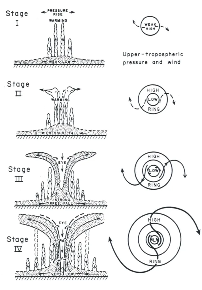
Fig. 1:The schematically evolution of a symmetrical tropical cyclone (TC) divided into four stages. The left side outlines the structure of a developing TC, whereas the right side shows the wind and pressure in the upper troposphere for a TC in the Northern Hemisphere (NH) (Palm´en and Newton, 1969).

(11)

1 Introduction

The development of TCs is not fully understood (Thatcher and Pu, 2011; Vecchi et al., 2013), although the description of tropical cyclogenesis as presented by Palm´en and New- ton (1969) is a widely accepted approximation. Correspondingly, the TC formation is split into four consecutive stages displayed in Fig. 1.

Stage I illustrates the transformation of atmospheric disturbance into a tropical depression, the weakest form of a TC. The intensification to a weak low-pressure system leads to convection of moist air, which triggers convective instability and thereby the formation of cumulonimbus clouds. In this process the rise of moist air releases latent heat and the temperature of the upper troposphere increases, which causes the pressure to rise aloft. As a consequence the air of the upper troposphere diverges and the surface pressure decreases.

The inflowing moist air strengthens resulting in higher wind velocities.

In Stage II the convection and the cyclonic circulation increase through the enhancement of the inward flow. This is associated with a reinforced convection and a higher release of latent heat, which further warms the troposphere from the upper center of the system downward and outward. There, the cyclonic vortex starts to form due to convective pro- cesses. In the upper troposphere around the vortex a high pressure ring develops from which the winds flow outward radially and a feeble low originates in the center of the ring.

The convective cumulonimbus clouds organize into spiral rain bands with the innermost spreading outward at the top to form the cirrus cloud shield (Fig. 2).

Stage III is characterized by the expansion of the upper cloud system and the downward evolution of the TC’s center, called the eye. The formation of the eye is caused by the elevation of air from lower levels with a strong cyclonic circulation to levels where in order to balance out the radial pressure gradient, the cyclonic rotation needs to be weaker or even anticyclonic. Since the air cannot rapidly adjust its strong cyclonic vorticity the air particles are deflected outward by the Coriolis and centrifugal force. The greater mass divergence in the upper troposphere is connected to a considerably faster fall of pressure in the central region. Within the eye, the descent of air leads to an adiabatic warming suppressing the clouds downward.

In Stage IV the formation reaches its climax in a mature TC with the final values of vertical mass circulation and of latent heat release. The cyclonic vorticity has strengthened so that air particles near the surface are unable to reach the center and the eye extents to the sea level.

The schematic structure of a mature TC, with its characteristic features, is illustrated in Fig. 2. The most remarkable feature of a mature TC is the eye in its center, which is nearly

(12)

Fig. 2:Structure of a mature TC in the NH (UCAR, 2010).

cloud-free. It is the region with the lowest pressure and has a typical size of 20−50 km.

The upper central region of the TC is up to 10°C warmer than the environment and forms the hot core. This is a result of the subsiding air in the eye releasing latent heat (Palm´en and Newton, 1969). Within the center of the eye, the winds are weak although they are increasing expeditiously outward reaching their maximum in the eyewall, which is associated with the strongest precipitation, pressure gradient and convection, near the surface.

There, the vertical winds can reach values of 5−10 m s^-1. The air spreads outward at the upper troposphere forming the cirrus cloud shield. The rain bands of convective clouds surround the eyewall spirally, occasionally touching it, and have the same direction as the inflow (Emanuel, 2003).

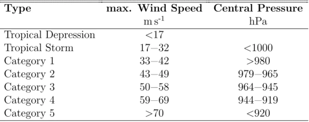
In Table 1 the Saffir–Simpson–Scale is illustrated. According to it TCs are scaled by their maximum sustained wind speed and central pressure. TCs with wind speeds above 32 m s^-1 are mature TCs which are broken down into five categories.

Table 1:Saffir–Simpson–Scale categorizes TCs by the maximum sustained wind speed and their central pressure (Kantha, 2006).

Type max. Wind Speed Central Pressure

m s^-1 hPa

Tropical Depression <17

Tropical Storm 17−32 <1000

Category 1 33−42 >980

Category 2 43−49 979−965

Category 3 50−58 964−945

Category 4 59−69 944−919

Category 5 >70 <920

(13)

1 Introduction

1.1 Tropical Cyclones in a Changing Climate

An issue, that has been addressed in several studies, is how frequency and intensity of TCs have changed or will change in a CO₂–warmed climate (e.g., Webster et al., 2005;

Latif et al., 2007; Emanuel, 2008; Emanuel et al., 2008; Kim et al., 2014). A review of studies is given by Knutson et al. (2010) which summarizes a presumed global decrease in TC frequency of −6 to −34 %, while TC intensity is supposed to increase by +2 to +11 % due to the greenhouse warming in the future. This increase in TC intensity is also supported byElsner et al. (2008). They examined observational data for the years 1981 to 2006 and showed a positive trend in the activity of the strongest TCs (categories 4 and 5).

Although the results of some studies are conflicting, Webster et al. (2005) suggested that observational data show an increase in the frequency of TC with hurricane strength in the North Atlantic during 1970 and 2004 related to a statistically significant positive trend of SST. The correlation between the SST and TC activity has been statistically significant over the past 50 years, especially in the North Atlantic (Goldenberg and Shapiro, 1996;

Emanuel, 2003, 2008;Knutson et al., 2010;IPCC, 2014). Bengtsson et al.(2007a) expounds that, although the spatial distribution of the tropical SST is an essential component of understanding TCs, it would be deceiving to exclusively consider SST regarding TC activity.

In contrast toWebster et al.(2005),Kim et al.(2014) suggest a negative trend of simulated TC activity in the North Atlantic (−30 %) caused by CO₂ doubling in general agreement with other studies (Held and Zhao, 2011;Knutson et al., 2010, 2013).

The challenge of detecting climate changes in TC activity from observational data is to ascertain whether changes in TC frequency are caused by natural variability or by specific climate forcings like aerosols or CO2 concentration. This uncertainty depends on the limitations of TC observations in the pre-satellite era (before 1966). In order to correct the historical records an approximated number of undetected TCs, due to ship-reportings, are added. After this adjustment, Knutson et al. (2010) show that the significant positive trends are greatly reduced. Additionally, this positive trend consists mainly of an increase in short duration TCs (<2 days), which is mostly associated with observational changes (Knutson et al., 2010). Therefore, an increase in long-term observational TC activity has a low confidence (IPCC, 2014).

The correlation of TC activity to certain large-scale environments like SST, static stability, vertical wind shear or relative humidity has been suggested in several studies (e.g., Goldenberg and Shapiro, 1996; Emanuel, 2003). An alternative to the direct analysis of observed or simulated TCs is to determine how large-scale environmental parameters are affected by climate change. How an increase of vertical wind shear in the North Atlantic can inhibit TC development is yielded by the El Ni˜no – Southern Oscillation (ENSO), a tropical circulation pattern which is associated with an ascent in vertical winds over the Western Pacific followed by a rise of vertical wind shear in the North Atlantic (Bengtsson

(14)

et al., 2007a,b; Goldenberg and Shapiro, 1996). Tang and Neelin (2004) suggested that the stability in the North Atlantic is also linked with the ENSO. In a warming climate, static stability is supposed to increase and this could cause the specific humidity to rise (Bengtsson et al., 2007b). Those effects are counteracting since a more stable troposphere would be detrimental for TC genesis, whereas humidity is advantageous. Kim et al.(2014) could not single out an individual variable that caused a significant global response of TCs despite the suggestion, that the inhomogeneous spatial changes of the environments could explain the response of simulated TCs on a sub-basin scale.

1.2 Research Motivation

TCs are among the most destructive natural disasters and the most lethal geographical hazards after floods (Emanuel, 2003;Emanuel et al., 2008). Therefore understanding how tropical cyclogenesis is affected by a warming climate is important not only scientifically but in terms of social economy (Camargo et al., 2007). As mentioned in the previous section, large-scale environmental factors like vertical wind shear, latent heat flux, stability and SST impact the development of TCs. However, the individual impacts are hard to distinguish.

This study addresses the question as to how large-scale environmental variables are affected by a doubling CO2 concentration in the Kiel Climate Model (KCM) and what consequences this implies for TC development. Further, a focus is set on the correlation between the seasonal cycles of the environmental parameters and the TC frequency.

(15)

2 Data and Methods

2.1 Data

2.1.1 Kiel Climate Model

In this thesis the model output from the Kiel Climate Model (KCM) (Park et al., 2009) was analyzed. The KCM is based on the Hamburg atmospheric general circulation model version 5 (ECHAM5) (Roeckner et al., 2003) and Nucleus for European Modeling of the Ocean (NEMO) (Madec, 2008). ECHAM5 and NEMO are coupled with the Ocean Atmosphere Sea Ice Soil version 3 (OASIS3) (Valcke, 2013) once per day, without any form of flux

Fig. 3:Structure of the main components of the KCM (Park et al., 2009).

correction (Fig. 3).

ECHAM5 is an atmospheric general circulation model (AGCM) developed at the Max Planck Institute for Meteo- rology (MPI). The atmospheric model used in the KCM has a horizontal resolution of T31 (3.75°× 3.75°) with 19 vertical levels up to 10 hPa.

NEMO consists of the Louvain-la- Neuve Ice Model version 2 (LIM2) and the ocean general circulation model (OGCM) Océan Parallélisé version 9

(OPA9). The NEMO version of the KCM has a resolution of 2°horizontally with an equa- torial latitudinal refinement to 0.5° and 31 vertical levels (Ding et al., 2015). A detailed description of the KCM is given by Park et al.(2009).

Two experiments from the KCM are analyzed in this study. One is the multi-millennial control run with a constant CO₂ concentration (348 ppm), hereafter twentieth-century equivalent (20C) run and the other consists of 22 global warming experiments, hereafter twenty- first-century equivalent (21C), each 100 years long with differing oceanic and atmospheric initial conditions taken from the 20C control run. The CO₂ concentration increases at a rate of 1 % per year in the 21C global warming run, CO₂ doubling is reached after 70 years, and thereafter the CO₂ concentration is stabilized for the last 30 years. This rate of increase is close to the observed current rate (Park et al., 2009; Bordbar et al., 2015).

In this thesis, the 20C control experiment was split into 22 segments with the same start values as the 21C global warming runs. The 20C control run reflects the climate without varying external forcing, whereas the 21C global warming experiment measures the signal forced through the CO₂ increase. The internal variability is indicated by the ensemble

(16)

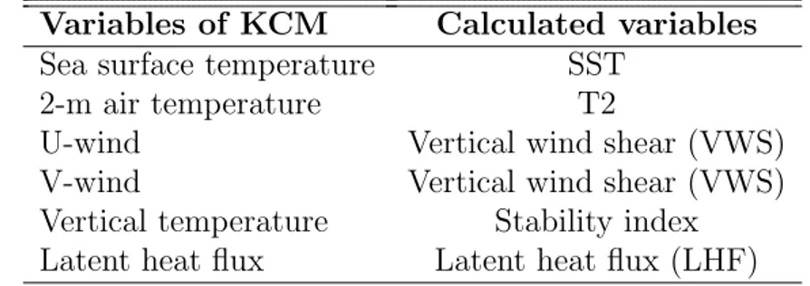
Table 2:The variables of the KCM which were used to analyze the environmental conditions affecting TC formation.

Variables of KCM Calculated variables Sea surface temperature SST

2-m air temperature T2

U-wind Vertical wind shear (VWS)

V-wind Vertical wind shear (VWS)

Vertical temperature Stability index Latent heat flux Latent heat flux (LHF)

spread which is the variability of the ensemble mean (see Ensemble Integrations).

0 20 40 60 80 100 13

14 15 16 17 18 19

TIME (years) T2 in o C

Fig. 4:Global averaged 2-m air temperature (T2) of 22 runs from the global warming simulation (21C, light gray lines) and from the control (20C, dark gray lines). The 11-years running averaged ensemble mean of the global warming runs (21C, red thick line) and of the control (20C, blue thick line).

Monthly mean values are used from the KCM (Table 2) to ascertain large- scale environmental changes. To select a satisfying algorithm for detecting TCs in the simulation (e.g., Zhao et al., 2009; Kim et al., 2014; Knut- son et al., 2013) this temporal resolution (monthly mean data) is too low to detect simulated TCs.

The global mean 2-m air temperature (T2) from the KCM exhibits an increase for the 21C global warming experiments, whereas for the 20C control simulation no significant trend is seen in Fig. 4. The ensemble spread is

±0.18°C for the 20C control run and

±0.17°C for the 21C experiments. The rise of the temperature slows after 70 years, which corresponds to the stabilization of the CO₂ concentration in 21C.

2.1.2 IBTrACS

The International Best Track Archive for Climate Stewardship (IBTrACS) dataset (v03r08) consists of at least 12 datasets from different agencies, including but not exhaustive to all of the World Meteorological Organization (WMO) Regional Specialized Meteorological Center (RSMC), Tropical Cyclone Warning Center (TCWC) and other national agencies, thus providing a global distribution of TCs at 6-h intervals. For further detail see Knapp et al.(2010). This study concentrates on the recent 30-year period (1981-2010) to examine observed TCs, since previous periods are less reliable (Schreck et al., 2014).

(17)

2 Data and Methods

2.1.3 NCEP/ NCAR Reanalysis

The National Centers for Environmental Prediction/ National Center for Atmospheric Re- search (NCEP/ NCAR) Reanalysis 1 (Kalnay et al., 1996) is used to calculate the vertical wind shear and stability index. It is given on a 2.5°×2.5°spatial grid and has been available since 1941 with 17 pressure levels. For comparison with the KCM, monthly mean data are used and, for consistences IBTrACS, the period from 1981 to 2010 is selected.

The data available for the latent heat flux has a horizontal resolution of T62 (2.0°latitude

× 1.75° longitude) and is also provided by the NCEP/ NCAR Reanalysis 1. This dataset does not provide monthly mean data, so the daily values are averaged into monthly mean values prior to analysis.

2.1.4 ERSST.v4

The global monthly mean Extended Reconstructed Sea Surface Temperature, version 4 (ERSST.v4) dataset by the National Oceanic and Atmospheric Administration (NOAA) has a spatial resolution of 2°× 2° and starts in January 1854 and is described in detail by Huang et al.(2015).

This study compares the simulated seasonal cycle of the SST to the ERSST.v4 during the years 1981 to 2010.

2.2 Methods

2.2.1 Ensemble Integrations

An ensemble (from French: ensemble ˆ= together) can either be a combination of different models, called a multi-model ensemble, or a combination of computations produced with the same model for varying initial conditions, referred to as an initial condition ensemble and as used in this study. This method is common for climate projections to estimate model uncertainties due to internal variability of the climate system.

2.2.2 Standard Deviation

The standard deviation (σ) is a statistical tool to measure the variability of a dataset (Storch and Zwiers, 2001) and is computed as follows:

σ = v u u t

1 N −1

N

X

i=1

(X_i−µX)² (1)

(18)

Where X_i is the value of an ensemble member i,N the number of values andµX the mean value.

The ensemble spread is the standard deviation of the 22 simulations for each grid point.

2.2.3 Correlation Coefficient

To qualify the relation between two annual cycles the correlation coefficient is calculated according to Storch and Zwiers (2001).

R_XY = E[(X−µ_X) (Y −µ_Y)]

σ_X σ_Y (2)

Where E is the expectation and µX, µY the average of X and Y.

The correlation coefficient R is non-dimensional and has a range between −1 and 1.

R² is the coefficient of determination that presents the percentage of variability of one variable which accounts for the variation of the other one.

Unless otherwise noted the correlation coefficients between the NCEP/ NCAR reanalysis data and the KCM are computed for the first 30 years (F30) of the 21C global warming experiment since at that time the CO₂ concentrations are roughly similar.

2.2.4 Signal-to-Noise

The spatial distribution of the signal-to-noise ratio is used to investigate the significance of CO₂–forced signals. The signal-to-noise ratio is defined as the absolute value of the difference between the last 30 years (L30) and the first 30 years (F30) divided by their ensemble spread (Barnett et al., 1991).

S/N = |S_L30−S_F₃₀| σL30−F30

(3) This ratio can only have positive values and is dimensionless. The greater the values, the more significant they become indicating a more robust CO₂–induced signal.

2.2.5 Data Processing

This subsection focuses on how the datasets in Table 2 and their corresponding NCEP/

NCAR or ERSST.v4 datasets are processed. The following calculations are done for all 22 runs individually for both set of experiments with the KCM.

The sea surface temperature (SST) and 2-m air temperature are converted from Kelvin (K) to Celsius (°C).

(19)

2 Data and Methods

The zonal and meridional winds (U-wind, V-wind) are required to compute the vertical wind shear between 200 hPa and 850 hPa in ms^-1:

Vertical Wind Shear (VWS) = q

(U₂₀₀−U₈₅₀)²+ (V₂₀₀−V₈₅₀)² (4) The vertical levels 200 hPa and 850 hPa are selected since the 200–850-hPa wind shear represents the tropospheric-deep shear which affects the TCs, and for the purpose of comparison with other studies. (e.g., Aiyyer and Thorncroft, 2006; Camargo et al., 2007; Kim et al., 2014;Paterson et al., 2005)

The temperature is converted into the potential temperature θ (see Emanuel, 1994) and calculated as follows:

θ(p) =T (p) p0

p

R c_p

(5) T is the absolute temperature in K at pressurep. R = 278 J kg^-1K^-1 is the gas constant of dry air and cp = 1003 J kg^-1K^-1 the specific heat capacity at constant pressure.

The potential temperature is the temperature a parcel of air would have if adiabatically lowered to a reference pressure, here p₀ = 1000 hPa. ’Adiabatically’ refers to a thermo- dynamical process where no heat or matter is exchanged. This temperature conversion is important to compare temperatures of different levels with one another.

Subsequently, the stability index was computed on the basis of the difference of the potential temperature between 500 hPa and 850 hPa (Gray, 1968, 1979).

Stability Index =θ(500 hPa)−θ(850 hPa) (6) Since the values of θ(850 hPa), which are nearer to the ground, are greater than those of θ(500 hPa), the values of the stability index will be negative. The atmospheric stability is increasing when the difference between those two vertical levels is increasing.

There are two differing conventions for the latent heat flux depending on the perspective.

From a meteorological perspective, the latent heat flux is positive when the atmosphere is gaining energy associated with evaporation and negative when heat is transferred into the ocean (Earth surface). Whereas from a oceanographic view it is the other way around, so that evaporation would lead to a negative latent heat flux. For the purpose of this study, the meteorological convention is applied.

(20)

2.2.6 Trend Computation

To develop the trend distribution a simple linear regression is performed for every segment of the 20C and every run of the 21C experiment. The simple linear regression relates a depended variable Y linearly to an independent variable X with a length of n (Storch and Zwiers, 2001).

Yi =a0+a1Xi+i (7)

In this equation a0 and a1 are the regression coefficients and i ∈ [1, n] is the time. i

describes the error at the time i.

The values of the linear regression’s last and first 30 years (L30, F30) are averaged for every 100-year long segment. Afterwards the values of those averaged F30 are subtracted from the L30 ones. The results are represented in a histogram.

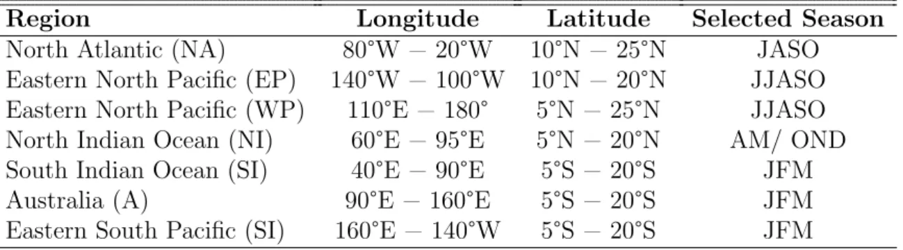
The trend distribution is produced individually for every region and selected season(s) (see Table 3).

(21)

3 Results

3.1 Tropical Belt

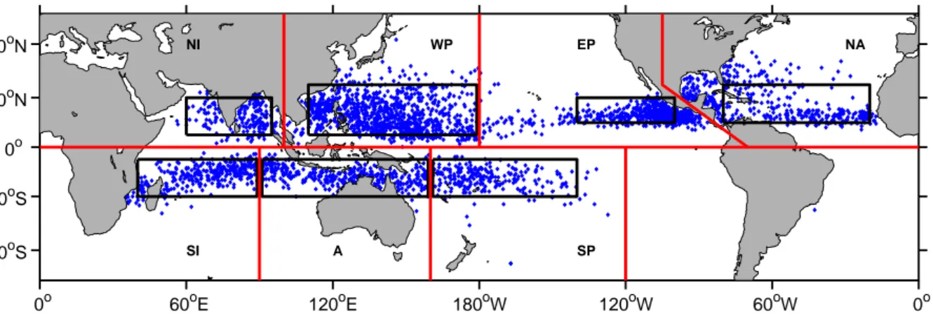
There are regions of the tropical ocean where TCs form more frequently than in others.

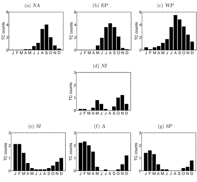
Figure 5 shows a map of the origin points of all TCs for the years 1981 to 2010. According to TC formation, the tropical ocean is subdivided into seven different regions: North Atlantic (NA), eastern North Pacific (EP), western North Pacific (WP), North Indian Ocean (NI), South Indian Ocean (SI), Australia (A) and eastern South Pacific (SP). These regions are defined by red lines in Fig. 5 and are only used for seasonal TC frequency, as illustrated in Fig. 6. The black boxes, which cover most of the TC genesis, circumscribe the selected development regions.

Due to strong vertical wind shear and comparatively low SSTs, TCs do typically not form over the eastern South Pacific and South Atlantic Gray (1979). Therefore, those regions are neglected hereafter.

The number of observed TCs is displayed for each region in Fig. 6. The annual cycle of TCs has a peak in the respective summer season for each hemisphere, except for the North Indian Ocean, which has a bimodal seasonal distribution (see Fig. 6d) with maxima in boreal spring and fall, as a result of the summer monsoon which is associated with strong vertical wind shear.

According to the peak TC seasons, the hemispheres are regarded separately for the global pattern of vertical wind shear and SST. The months June – October (JJASO) are selected for the boreal summer and January – March (JFM) for the austral summer.

Figure 7a shows the geographical distribution of vertical wind shear during the boreal

0ô 60ôE 120ôE 180ôW 120ôW 60ôW 0ô 40ôS

20ôS 0ô 20ôN

40^oN ^NI ^WP ^EP ^NA

SI A SP

Fig. 5:The blue dots display the observed origin of TCs for 1981/2010 from IBTrACS. Red lines indicate the basin devision for Fig. 6, black boxes represent the developing regions of TCs analyzed in this study (see Table 3).

(22)

(a)NA

J F M A M J J A S O N D 0

2 4 6

TC counts

(b) EP

2 4 6

TC counts

(c) WP

2 4 6

TC counts

(d)NI

1 2 3

TC counts

(e)SI

1 2 3

TC counts

(f) A

1 2 3

TC counts

(g)SP

1 2 3

TC counts

Fig. 6:The observed monthly TC frequency (yr^-1) of the seasonal cycle during 1981 to 2010 from Schreck et al.(2014) for seven regions: (a)North Atlantic,(b)eastern North Pacific,(c) western North Pacific, (d) North Indian Ocean, (e) South Indian Ocean, (f) Australia and(g) eastern South Pacific. Note that the y-axis values in(a)-(c)differ from those in (d)-(g).

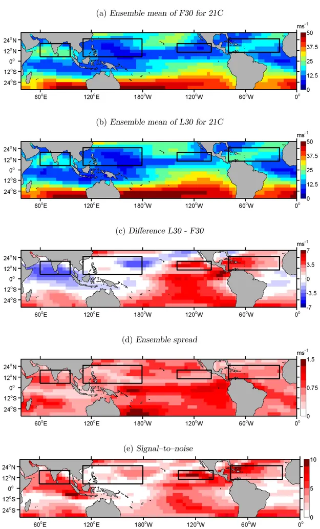
summer of the ensemble mean of the 21C global warming simulations for the first 30 years (F30). Figure 7b presents the last 30 years, respectively. The CO₂–induced change between the L30 and F30 affects the vertical wind shear in each of the NH regions differently (Fig. 7c). In the North Atlantic and the eastern North Pacific, vertical wind shear is in- creased by up to 6.3 ± 0.8 m s^-1 being detrimental for TC formation. In these two TC development regions, the signal-to-noise ratios are relatively high (Fig. 7e). Values up to 9 indicate that this trend is with very high confidence forced by the rising CO₂ concentration.

In the North Indian Ocean vertical wind shear is decreasing (Fig. 7c) but the absolute values are still relatively unfavorable for tropical cyclogenesis during JJASO (Fig. 7b). This is due to the monsoon season that lasts from June until September.

Within the western North Pacific the trend of vertical wind shear shows contrary results.

(23)

3 Results

On the east side of the development region, the vertical wind shear is decreasing and exceeds values of−4.3±0.9 m s^-1, whereas on the western side it is slightly increasing. The decrease is not only stronger but its signal-to-noise ratio is higher but not as much as in other regions.

Overall, this suggest a tendency beneficial to TC development.

Figure 8 yields the same structure as Fig. 7 and displays the vertical wind shear for the austral summer JFM. The South Indian Ocean trend bears a resemblance to the trend of the western North Pacific, having conflicting trends within the development region. As for the western North Pacific, the South Indian Ocean has a negative trend that covers a larger area with a stronger signal-to-noise ratio. A decreasing trend is also found for the Australian region, where the area of decrease is greater than for the South Indian Ocean and the signal-to-noise ratio is larger. The highest increase in the seven regions is found in the south eastern corner of the eastern South Pacific development region with values of 9.2

± 1.5 m s^-1 and high signal-to-noise ratio.

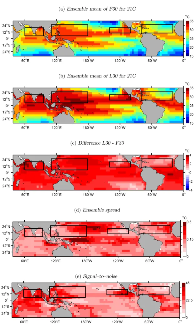
The spatial response pattern of the global SST is less complicated than the response of vertical wind shear (Fig. 9 and Fig. 10). The SST rises in the tropical region (30°N−30°S) by 2.14°C for the NH summer and 2.12°C for the austral summer. The lowest values of SST during the F30 with 22.2 ±0.2°C are found in the North Atlantic in the northeastern corner Fig. 9a. In this region vertical wind shear is also rather strong (19.5± 0.4 m s^-1) and the latent heat flux, another environmental factor for tropical cyclogenesis, has rather low values there (see Appendix Fig. 19a).

The horizontal distribution of the stability index and the latent heat flux are not further analyzed since their spatial structure does not exhibit any unexpected regional differences.

They are shown in the Appendix in Fig. 17 and Fig. 19 for the boreal summer and in Fig. 18 and Fig. 20 for the austral summer.

In the following sections of this chapter only three regions will be discussed in detail for convenience. The regions are the North Atlantic, North Indian Ocean and Australia, since they depict larger differences among each other.

Table 3:Domain circumscription and selected seasons used for regional integrations.

Region Longitude Latitude Selected Season North Atlantic (NA) 80°W − 20°W 10°N − 25°N JASO Eastern North Pacific (EP) 140°W − 100°W 10°N − 20°N JJASO Eastern North Pacific (WP) 110°E −180° 5°N −25°N JJASO North Indian Ocean (NI) 60°E − 95°E 5°N −20°N AM/ OND South Indian Ocean (SI) 40°E − 90°E 5°S −20°S JFM Australia (A) 90°E −160°E 5°S −20°S JFM Eastern South Pacific (SI) 160°E −140°W 5°S −20°S JFM

(24)

(a)Ensemble mean of F30 for 21C

(b) Ensemble mean of L30 for 21C

(c)Difference L30 - F30

(d)Ensemble spread

(e)Signal–to–noise

Fig. 7:Vertical wind shear between 200 hPa and 850 hPa during boreal summer (JJASO) for (a) the first 30 years (F30) and (b) the last 30 years (L30) of the 21C global warming

(25)

3 Results

(a) Ensemble mean of F30 for 21C

(b)Ensemble mean of L30 for 21C

(c) Difference L30 - F30

(d)Ensemble spread

:Same as Fig. 7, for austral summer (JFM).

(26)

(a)Ensemble mean of F30 for 21C

(b) Ensemble mean of L30 for 21C

(c)Difference L30 - F30

(d)Ensemble spread

Fig. 9:SST during boreal summer (JJASO) for (a) the first 30 years (F30) and (b) the last

(27)

3 Results

(a) Ensemble mean of F30 for 21C

(b)Ensemble mean of L30 for 21C

(c) Difference L30 - F30

(d)Ensemble spread

(28)

3.2 Seasonal Cycles in Selected Basins

(a)NA

10 20 30 40

VWS in ms−1

ensemble F30 ensemble L30

NCEP/NCAR 1981/2010

(b) NI

10 20 30 40

VWS in ms−1

(c) A

10 20 30 40

VWS in ms−1

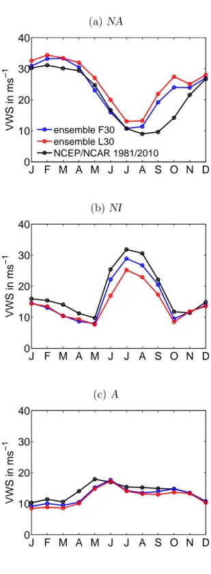
Fig. 11:The seasonal cycle of vertical wind shear (VWS) for three regions: (a) North Atlantic, (b) North Indian Ocean and(c)Australia. The blue and red line show the ensemble mean of the F30 and L30 for the 21C global warming experiment.

The black line depicts the NCEP/

NCAR reanalysis data during 1981

In this section the annual cycles of the stability index, latent heat flux and vertical wind shear are discussed for the areas North Atlantic, North Indian Ocean and Australia. Figure 11 displays the annual cycle of vertical wind shear for the F30 and L30 of the KCM, and the NCEP/

NCAR data of the years 1981 to 2010.

The best resemblance between the model simulations and the NCEP/ NCAR reanalysis data is found for the North Indian Ocean (R_{N I} = 0.99) although most KCM values are somewhat lower (Fig. 11b). For the North Atlantic and Australia, the resemblance is also respectable (R_{N A} = 0.90, R_A= 0.89) (Fig. 11a, (c)).

In the North Atlantic the vertical wind shear starts to strengthen again after August for both 21C periods with the KCM, whereas the NCEP/

NCAR only starts to rise after September. In contradiction to the other regions, the vertical wind shear values of the KCM are partly higher than those from NCEP/ NCAR. In the North Atlantic the vertical wind shear values for L30 are above those of the F30 for every month. For comparison with the seasonal cycle of TC activity, (Fig. 6) the correlation coefficients between the annual cycles of the vertical wind shear and TCs counts are computed (Table 4).

The NCEP/ NCAR reanalysis data are better correlated with the annual cycle of the monthly TC frequency in the North Atlantic than the ensemble means of the KCM. The correlation for the NCEP/ NCAR with the TC frequency is R=−0.85. The KCM only has a correlation of R = −0.62, due to the too early rise of vertical wind shear.

The North Indian Ocean is exceptional as a result of the monsoon season and depicts the high-

(29)

3 Results

Table 4:Correlation coefficients between the monthly mean seasonal cycles of the vertical wind shear (Fig. 11) and TC frequency (Fig. 6) are displayed for three regions: North Atlantic (NA), North Indian Ocean (NI) and Australia (A). For the vertical wind shear there are three different annual cycles: the first 30 years (F30) and last 30 years (L30) of the 21C global warming simulation and NCEP/ NCAR during 1981 to 2010.

NA NI A

F30 of 21C −0.62 − 0.43 − 0.90

L30 of 21C −0.62 − 0.49 − 0.91

NCEP/ NCAR (1981/2010) −0.85 − 0.50 − 0.83

est vertical wind shear during the boreal summer (Fig. 11b). The lowest vertical wind shear is found in May and October for the KCM which correlates with the months depicting the most TCs. However, the correlation between the seasonal cycles of vertical wind shear and the TC activity is R = −0.50 for NCEP/ NCAR and even lower for the KCM. This indicates that the vertical wind shear does not capture well the seasonal TC distribution for the North Indian Ocean (Table 4). For the months June to September, the vertical wind shear of the L30 decreases compared to the F30.

In Australia, the increase of vertical wind shear that is seen from March to May in NCEP/

NCAR, is shifted in the KCM to April to June (Fig. 11c). Within the Australian region, the monthly mean vertical wind shear does not exceed values of 18 m s^-1, thereby having generally weaker vertical wind shear than the other seven regions (see Appendix Fig. 21).

From December to March, the wind shear is the weakest with a good anti-correlation to the TC counts (see Table 4).

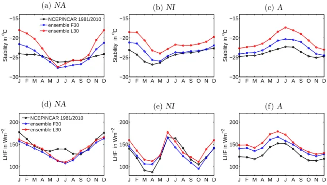
An unstable atmosphere is favorable for TC formation. In the North Atlantic development region the KCM’s stability index is well correlated with NCEP/ NCAR (RN A= 0.97) but exhibits larger seasonal amplitudes (Fig. 12a). The least stable months are from June to September. In Fig. 12d, the latent heat flux bias of the KCM is largest during boreal summer. During winter the latent heat flux is stronger because the temperature difference between the ocean and atmosphere is greater. From July – October, the relevant months for TC genesis, both the latent heat flux and stability index increase. However, these two environmental factors have opposing effects on tropical cyclogenesis: An increase of latent heat flux leads to an increase in available energy for TC formation, whereas an increase of the stability index leads to less convection and could inhibit TC genesis.

The stability index of the North Indian Ocean (Fig. 12b) does not have a bimodal shape and is therefore an exception from the other environmental factors (see Fig. 11b, Fig. 12e, Appendix Fig. 23d). This results in relatively low correlations with the annual cycle of the TC counts. It is interesting that the correlation coefficients of the KCM control run and F30 of the 21C simulation have opposite signs (R_KCM = 0.24, R_F₃₀ = −0.17). The stability index between the NCEP/ NCAR and the KCM has the lowest correlations in

(30)

the three regions analyzed for all environmental variables. Before the monsoon season, the stability index decreases and reaches its minimum from April – May (AM) in NCEP/

NCAR (Fig. 12b). This also corresponds to one of the vertical wind shear minima.

The months October – December (OND) are the post-monsoon season, where the second minimum of vertical wind shear is situated. The stability index shows no minimum there.

The atmospheric stability increases for the L30 over the entire seasonal cycle. In contrast to the stability index, the latent heat flux of the North Indian Ocean is well correlated with the NCEP/ NCAR (R_KCM = 0.89) and presents two peaks in April and October which both are followed by an abrupt increase (Fig. 12e) and fairly high values in May and from November to December where the seasonal cycle of the TCs has its maxima. With rising CO₂ the atmosphere gains more latent heat during OND, which could support TC formation.

In Australia the correlation of the stability index with NCEP/ NCAR is R_A = 0.93 and for the latent heat flux it is RA = 0.95, implying that the KCM approximates the data.

An offset for both variables is obvious. The stability index displays no strict minimum for the months JFM which are related to TC events (Fig. 12c). There is a minimum during October and November, which is also seen in the latent heat flux although it cannot be detected for the vertical wind shear or SST (see Appendix Fig. 23f). The KCM, which is not indicating this minimum, has a greater correlation coefficient (R = −0.77) with the TC formation than the NCEP/ NCAR (R =−0.61). In general, the latent heat flux will

(a) NA

J F M A M J J A S O N D

−30

−25

−20

−15

Stability in oC

NCEP/NCAR 1981/2010 ensemble F30 ensemble L30

(b)NI

−30

−25

−20

−15

Stability in o C

(c) A

−30

−25

−20

−15

Stability in oC

(d)NA

150 200

LHF in Wm−2

NCEP/NCAR 1981/2010 ensemble F30 ensemble L30

(e)NI

150 200

LHF in Wm−2

(f)A

150 200

LHF in Wm−2

Fig. 12:Same as Fig. 11, but for stability index between 500 hPa and 850 hPa (Stability,(a)−(c)) and for latent heat flux (LHF,(d)−(f)).

(31)

3 Results

rise through CO₂–induced global warming, which could have a positive effect on tropical cyclogenesis.

The seasonal cycles for all seven regions are displayed in the Appendix (Fig. 21, Fig. 22, Fig. 24), including the not analyzed annual cycles of the SST in Fig. 23.

To further examine the CO₂–forced signal several time series will be presented in section 3.3. The vertical wind shear has the greatest correlation coefficients with the TC activity. Therefore to select seasons which are relevant for TC development the main crite- rion is the vertical wind shear with a particular focus on the NCEP/ NCAR reanalysis data and TC counts. For the North Atlantic months with at least one TC event and vertical wind shear values below 15 m s^-1 are chosen, i.e. the months July – October (JASO). The months JFM are singled out for Australia in a similar manner, but only vertical wind shear values below 12 m s^-1 are selected since the vertical wind shear in this region is generally lower than in the others. December is left out since, it is not signaling a difference between F30 and L30. Taking the bimodal structure of the North Indian Ocean into account, there are two periods selected which have at least 0.5 TC counts and vertical wind shear values below 15 m s^-1. Those are AM for the pre-monsoon season and OND for the post-monsoon (also shown in Tropical Belt Table 3).

3.3 Trend Analysis

The development of the vertical wind shear and the latent heat flux over time (100-year period) in the 21C climate will be discussed in this section as well as the trend distributions of the 20C and 21C simulations. To calculate the trend distribution the averaged L30 and F30 of the linear trend from the 22 segments for each experiment are subtracted. For further detail see Trend Computation.

The evolution of the vertical wind shear from the 21C global warming simulation is shown in Fig. 13 for the previously selected seasons for the regions North Atlantic, Australia and North Indian Ocean.

The vertical wind shear development for the months JASO is increasing within the North Atlantic over the 100-year period as well as the variability (Fig. 13a). The standard deviation (σ) never exceeds values of ±2.36 m s^-1. To determine if the increasing trend is significant Fig. 14a is analyzed. This histogram of trends for the 20C and 21C experiments shows two isolated distributions of trends of 22 segments for the North Atlantic, thus providing evidence of a CO₂– forced increase in vertical wind shear, since internal variability is not able to explain this increase. The averaged trend for the control simulation (20C) is −0.06±0.34 m s^-1, whereas for the 21C it is 2.55±0.45 m s^-1 leading to a vertical wind shear increase of 2.61±0.45 m s^-1 (Table 5). This rise of the vertical wind shear would be

(32)

(a)NA for JASO

0 20 40 60 80 100 10

15 20 25 30

TIME (years)

VWS in ms−1

(b) A for JFM

0 20 40 60 80 100 5

10 15

TIME (years)

VWS in ms−1

(c)NI for AM

0 20 40 60 80 100 0

5 10 15 20

TIME (years)

VWS in ms−1

(d)NI for OND

0 20 40 60 80 100 0

5 10 15 20

TIME (years)

VWS in ms−1

Fig. 13:Development of vertical wind shear (VWS) for the 22 annual values of the 21C experiments (thin gray lines) for four regions: (a) North Atlantic for the months July – October,(b)Australia for the months January – March,(c)North Indian Ocean for the months April – May and(d) North Indian Ocean for the months October – December.

The red thick line represents the ensemble mean with an 11-years running mean filter and the bars the 1 standard deviation range. Note the different y-axis values.

detrimental for TCs and could reduce the TC frequency in the North Atlantic in the future.

Since the standard deviation exceeds by far the mean trend of the 20C control segments for each region (Table 5) the 20C experiment trend is not significant thereby indicating that the increase of vertical wind shear in the 21C climate is induced by higher values of CO₂.

In contrast to the North Atlantic, the vertical wind shear in Australia is decreasing. The ensemble spread (Fig. 13b) has the highest values at 15 years (σ = 1.8 m s^-1) and the lowest at 95 years (σ = 0.74 m s^-1). Figure 14b is considered to yield an estimate of how significant the decreasing trend of Australia is in the 21C global warming simulation. The trend distribution of the two simulations is not clearly disjunct, although the overlapping area is relatively small and only one of the 20C control segments overlaps the distribution of the global warming simulation. Overall, there is a decreasing trend of the vertical wind shear for Australia (−0.97±0.28 m s^-1), which is a smaller alteration compared to that of the North Atlantic. Nevertheless the impact on TCs could be stronger, since the initial absolute values of vertical wind shear for the ensemble mean (9.69 m s^-1 at 6 years) are

(33)

3 Results

(a) NA for JASO

0 1 2 3

0 2 4 6 8 10 12

VWS in ms⁻¹

Number of trends

20C 21C

(b)A for JFM

−1.50 −1 −0.5 0 0.5

2 4 6 8 10 12

VWS in ms⁻¹

Number of trends

20C 21C

(c)NI for AM

−1 −0.5 0 0.5 1

0 2 4 6 8 10 12

VWS in ms⁻¹

Number of trends

20C 21C

(d)NI for OND

−1 −0.5 0 0.5 1

0 2 4 6 8 10 12

VWS in ms⁻¹

Number of trends

20C 21C

Fig. 14:Distribution of 22 segments for each simulation of vertical wind shear differences for the 20C control experiments (blue) and the 21C global warming simulations (red) for four regions: (a)North Atlantic for the months July – October,(b)Australia for the months January – March, (c) North Indian Ocean for the months April – May and (d) North Indian Ocean for the months October – December.

already slightly below 10 m s^-1 (values above could limit TC formation), and a further decrease could enhance the number of TCs .

In the North Indian Ocean the ensemble spread strengthens for the pre-monsoon season (AM) (σ = 1.95 m s^-1at 25 years,σ= 2.61 m s^-1at 95 years) although the vertical wind shear remains stationary (Fig. 13c). Additionally the trend distributions are strongly overlapping (Fig. 14a) and the mean trend values are smaller than the according spread (see Table 5), Table 5:Averaged trend values of the vertical wind shear distributions for the 20C and 21C simulations with their standard deviation in m s^-1 (Fig. 14). The increase is calculated as the difference of the two simulations with the highest spread.

NA NI A

AM OND

20C −0.06±0.34 −0.02±0.48 −0.03±0.46 0.04±0.28 21C 2.55±0.45 0.19±0.42 −0.41±0.51 −0.93±0.25 Increase 2.61±0.45 0.21±0.48 −0.38±0.51 −0.97±0.28

(34)

(a)NA for JASO

0 20 40 60 80 100 100

120 140 160 180

TIME (years)

LHF in Wm−2

(b) A for JFM

0 20 40 60 80 100 100

120 140 160 180

TIME (years)

LHF in Wm−2

(c)NI for AM

0 20 40 60 80 100 100

120 140 160 180

TIME (years)

LHF in Wm−2

(d)NI for OND

0 20 40 60 80 100 100

120 140 160 180

TIME (years)

LHF in Wm−2

Fig. 15:Same as Fig. 13, for latent heat flux.

which implies that the trend is not significant. Hence the TC frequency would remain unchanged based on the vertical wind shear.

With a few exceptions, the post-monsoon season (OND) resembles the months JFM of the North Indian Ocean. The most remarkable difference is the generally stronger vertical wind shear (Fig. 13d), whose mean for OND is 11.41±1.68 m s^-1 compared to 8.31±2.23 m s^-1 for JFM. The variability is another difference as it has no distinct tendency and is weaker on average.

The development of the latent heat flux is globally increasing though there are regional differences (see Fig. 15, Appendix Fig. 29). The ensemble of the 20C simulations of the latent heat flux again does not exhibit any significant trend (Table 6) so that a trend seen in the 21C experiment is CO₂–forced.

The latent heat flux of the North Atlantic is only slightly ascending but its standard deviation is the smallest for the four regions analyzed (Fig. 15). Although this trend is comparatively weak the distributions of the 20C control and 21C global warming experiment are well separated (Fig. 16a). Latent heat flux rises 4.87±0.97 W m^-2 in response to a doubling of the CO₂ concentration (Table 6).

(35)

3 Results

(a)NA for JASO

−2 0 2 4 6

0 2 4 6 8 10 12

LHF in Wm⁻²

Number of trends

20C 21C

(b)A for JFM

−3−2−1 0 1 2 3 4 5 6 7 8 9 10 0

2 4 6 8 10 12

LHF in Wm⁻²

Number of trends

20C 21C

(c)NI for AM

−2 0 2 4 6

0 2 4 6 8 10 12

LHF in Wm⁻²

Number of trends

20C 21C

(d) NI for OND

0 5 10 15 20

0 2 4 6 8 10 12

LHF in Wm⁻²

Number of trends

20C 21C

Fig. 16:Same as Fig. 14, for latent heat flux changes.

A stronger increase of the latent heat flux is found for Australia accompanied by a stronger variability (Fig. 15b). Albeit this increase cannot be explained by internal variability for Fig. 16b exhibits, the well separated distributions for the two KCM ensembles would lead to a moister middle troposphere supporting TC genesis.

The post-monsoon season (OND) of the North Indian Ocean features an exceptional increase of latent heat flux (Fig. 15d) and an ensemble spread which is similar to that of Australia.

The averaged trend of the 21C runs shows a pronounced increase of 17.00±1.89 W m^-2 (Table 6). Furthermore in Fig. 15d the rate of latent heat flux increase slows after 70 years as the CO₂ concentration is stabilized. The trend distribution displays a wide gap between

Table 6:Same as Table 5, for latent heat flux in W m^-2

NA NI A

AM OND

20C −0.30±0.91 −0.32±1.57 0.04±1.31 0.12±0.97 21C 4.57±0.97 3.67±1.94 17.04±1.89 7.23±1.05 Increase 4.87±0.97 3.99±1.94 17.00±1.89 7.11±1.05

(36)

the 20C and 21C climates (Fig. 16d), which suggests a positive impact on TC development.

In contrast to that, in the pre-monsoon season (JFM) the latent heat flux is only weakly increasing, and the ensemble spread of the latent heat flux in the North Indian Ocean is the strongest of all seven regions (see Fig. 15c, Appendix Fig. 29). Thus the trend distributions are overlapping. The tropical cyclogenesis during this time would show a feeble effect.

The investigated evolutions and trend distribution of the vertical wind shear and the latent heat flux for all seven regions are illustrated in the Fig. 25, Fig. 26, Fig. 29 and Fig. 30 in the Appendix. For the stability and the SST only the time series are shown (Fig. 27, Fig. 28 ).

(37)

4 Discussion

This chapter is divided into two sections. In the first section the results of the preceding chapter will be discussed and compared to previous studies. Afterwards the outlook will provide a suggestion on how to improve the methods of this study in further investigations.

4.1 Comparison of Results

The main purpose of this thesis was to explore the influence of a CO₂ doubling on environmental conditions in the tropical belt and what consequences this may have on TC development.

In the first section of Results, the spatial distribution of two environmental parameters within the tropical belt were examined.

The vertical wind shear during the boreal summer (JJASO) increases in the North Atlantic and eastern North Pacific, and decreases in the North Indian Ocean and western North Pacific in response to a CO₂ increase. This increase in vertical wind shear between 200 hPa and 850 hPa is also seen inKim et al. (2014) as well as the decrease over the North Indian Ocean and the western North Pacific, though the KCM produces higher magnitudes for the increase and the decrease. The most distinct change of vertical wind shear from the KCM is found over the western corner of the eastern North Pacific with 6.3 m s^-1, whereas the strongest increase of vertical wind shear within the eastern North Pacific forKim et al.

(2014) is found near the east coast of Mexico where the vertical wind shear only reach values up to 2.5 m s^-1. The response of vertical wind shear for the North Atlantic increases strongly over the Caribbean islands. A similar pattern for the vertical wind shear is found byKnutson et al.(2013). However, a difference of vertical wind shear is found for the North Atlantic byKim et al.(2014), while the decreasing trends over the North Indian Ocean and western North Pacific correspond. These differences might be an effect of differing months used for the boreal summer.

For the austral summer (JFM) the vertical wind shear of the KCM decreases over the South Indian Ocean, Australia and the western South Pacific, and increases over the eastern South Pacific. The comparison of the results with Kim et al. (2014) yields some contradicting signals. In the South Indian Ocean and the western South Pacific there is an increase of vertical wind shear, whereas in the western South Pacific the vertical wind shear exceeds values of +2.5 m s^-1, on the contrary the vertical wind shear of this study suggest a negative trend in this region of−7.5 m s^-1. These contrasting evolutions in the western South Pacific of vertical wind shear could be explained by the positive bias in the model used by Kim et al.(2014). However, the general conditions for TC genesis are unfavorable in the western

(38)

South Pacific.

In Australia the KCM presents a slight decrease of vertical wind shear, while there is no significant trend displayed in the paper of Kim et al. (2014). Their model indicates a positive bias in this region which could explain the absence of this outcome.

Both studies show consistent trends for the regions North Atlantic, eastern North Pacific, western North Pacific, North Indian Ocean and the eastern South Pacific. This entails that the level of confidence rises in those regions concerning the vertical wind shear. If all other environments were unchanged, an increase of vertical wind shear would be detrimental for tropical cyclogenesis. This is the case for the regions North Atlantic, eastern North Pacific and eastern South Pacific. Zhao et al.(2009) point out that the correlation between the vertical wind shear and TC development does not imply that the influence on TCs is dominant. However, a strong vertical wind shear can inhibit the TC development against other supporting conditions.

This study’s changes in the SST, which shows a less complex spatial structure than the vertical wind shear, resemble the features of the study from Kim et al. (2014) during the boreal summer. In the North Atlantic the SSTs of both studies have a negative bias with roughly the same magnitude (Kim et al., 2014; Park et al., 2009). The simulated SSTs are too cool, which is a typical problem in the North Atlantic (Park et al., 2009). In the austral summer the SSTs of the development regions are consistent with Kim et al. (2014).

In section 3.2, the seasonal cycles of the three environmental variables vertical wind shear, stability and latent heat flux were examined for three regions North Atlantic, North Indian Ocean and Australia. One part of the analysis is to determine how well the environmental variables correlate to NCEP/ NCAR to detect seasonal model biases. The other part deals with the correlation between the seasonal cycle of TC counts and of the environmental parameters.

A correlation between the NCEP/ NCAR seasonal cycle of vertical wind shear and TC frequency is found for the North Atlantic and Australia. The connection between the observed seasonal cycle of vertical wind shear and TCs was also evaluated by Aiyyer and Thorncroft (2006) for the years 1958 to 2003. They concluded that the vertical wind shear over the North Atlantic (7.5°N−20°N, 85°W−15°W) during JASO cannot solely account for the TC formation. Vertical wind shear values for August and September are very close, but the TC count registrates far more individual TCs in September than in August.

This generally corresponds with the results of this study, although the increase of TC frequency from August to September is not as substantial. This could be caused by several differences in the comparison. One is that in this study TCs of the entire North Atlantic are consulted, whereas Aiyyer and Thorncroft (2006) only counted those within their selected development region which leads to a lower number of TCs. Another reason might be that they chose a time period which also includes years of the pre-satellite era. Thus these