Ecohydrographic control on the community structure and vertical distribution of pelagic Chaetognatha in the Red Sea
Item Type Article
Authors Karati, Kusum Komal; Al-Aidaroos, Ali M.; Devassy, Reny P.; El- sherbiny, Mohsen M.; Jones, Burton; Sommer, Ulrich; Kürten, Benjamin
Citation Karati KK, Al-Aidaroos AM, Devassy RP, El-Sherbiny MM, Jones BH, et al. (2019) Ecohydrographic control on the community structure and vertical distribution of pelagic Chaetognatha in the Red Sea. Marine Biology 166. Available: http://dx.doi.org/10.1007/
s00227-019-3472-x.
Eprint version Post-print
DOI 10.1007/s00227-019-3472-x
Publisher Springer Nature
Journal Marine Biology
Rights The final publication is available at Springer via http://
dx.doi.org/10.1007/s00227-019-3472-x Download date 07/05/2021 12:38:25
Link to Item http://hdl.handle.net/10754/630971
Ecohydrographic control on the community structure and vertical distribution of pelagic 1
Chaetognatha in the Red Sea 2
3
Kusum Komal Karati1,2*#, Ali M. Al-Aidaroos3, Reny P Devassy3, Mohsen M. El-Sherbiny3, 4, 4
Burton H. Jones5, Ulrich Sommer6, Benjamin Kürten5*, 6 5
Affiliations 6
1 CSIR -National Institute of Oceanography, Regional Centre Kochi, Kochi 682018, India 7
2 Centre for Marine Living Resources and Ecology, Kochi, 682037, India, * present address 8
3 King Abdulaziz University, Department of Marine Biology, Faculty of Marine Sciences, P.O.
9
Box 80207, Jeddah 21589, Kingdom of Saudi Arabia 10
4 Suez Canal University, Department of Marine Science, Faculty of Science, Ismailia 41522, 11
Egypt 12
5 King Abdullah University of Science and Technology (KAUST), Red Sea Research Center 13
(RSRC), Biological and Environmental Sciences & Engineering Division (BESE), Thuwal, 14
23955-6900, Saudi Arabia, * present address 15
6 GEOMAR Helmholtz Centre for Ocean Research Kiel, Marine Ecology, Düsternbrooker Weg 16
20, 24105 Kiel, Germany 17
18
#Correspondence to: Kusum Komal Karati 19
Email: kusum.kk1@gmail.com 20
Phone: +919895305666 21
ORCID IDs 22
KK orcid.org/0000-0001-9627-7466 23
BK orcid.org/0000-0003-0328-7847 24
BHJ orcid.org/0000-0002-9599-15 25
Disclosure statement 26
BK and AA conceived the study. BK, ME, RD and AA carried out fieldwork, analyzed the 27
zooplankton samples, and processed the data. KK provided taxonomic identifications of 28
Chaetognatha, interpreted the data, and drafted the manuscript. BK, US, and BJ provided 29
editorial advice.
30
Revised Manuscript Click here to access/download;Manuscript;Revised
Manuscript.docx Click here to view linked References
2 Abstract
31
The present study details the effects of basin-scale hydrographic characteristics of the Red Sea 32
on the macroecology of Chaetognatha, a major plankton component in the pelagic realm. The 33
hydrographic attributes and circulation of the Red Sea as a result of its limited connection with 34
the northern Indian Ocean make it a unique ecohydrographic region in the world ocean. Here, we 35
aimed to identify the prime determinants governing the community structure and vertical 36
distribution of the Cheatognatha in this ecologically significant world ocean basin. The intrusion 37
of Gulf of Aden Water influenced the Chaetognatha community composition in the south, 38
whereas the overturning circulation altered their vertical distribution in the north. The existence 39
of hypoxic waters (<100 µmol kg -1) at mid-depth also influenced their vertical distribution. The 40
detailed evaluation of the responses of the different life stages of Chaetognatha revealed an 41
increased susceptibility of adult individuals to hypoxic waters compared to immature stages.
42
Higher oxygen demands of the adults for the egg and sperm production might have prevented 43
them from inhabiting the oxygen deficient mid-depth zones. The carbon and nitrogen content of 44
the Copepoda and Chaetognatha communities and the quantification of the predation impact of 45
Chaetognatha on Copepoda based on the feeding rate helped in corroborating the significant 46
trophic link between these two prey-predator taxa. The observed influences of physical and 47
chemical attributes on the distribution of Chaetognatha can be used as a model example for the 48
role of the hydrography on the zooplankton community of the Red Sea.
49
Keywords: Biogeography; Chaetognatha; Ecohydrography; Macroecology; Red Sea;
50
Zooplankton 51
52 53
3 Introduction
54
The phylum Chaetognatha embraces a major component of pelagic plankton in the global oceans 55
and their marginal seas (Nair 1978; Bohata and Koppelmann, 2013; Terazaki 2013; Kürten et al.
56
2014). As carnivores, chaetognaths are known to consume ~1 to 12 prey day-1 ranging from 57
oligotrophic to productive environments (Kimmerer 1984; Kehayias 2003) and therefore play a 58
pivotal role in the trophodynamics of marine ecosystems. Their sensitivity to the physical and 59
chemical environment leading to their association with specific water masses makes them 60
suitable bioindicators of ecohydrographic provinces (Nagai et al. 2006; Buchanan and Beckley 61
2016) and for regions with increased primary productivity and the underlying physical processes 62
(e.g. eddies, fronts, and upwelling) (Kusum et al. 2014; Lima 2014; Nair et al. 2015).
63
The Red Sea, geographically positioned between the Asian and African continents and 64
characterized by an area of 4.51 × 10⁵ km2 and a length of ~2000 km is a semi-enclosed inlet of 65
the Indian Ocean (Sofianos and Johns 2002). The high evaporation rates (>2 m yr-1), low 66
precipitation (0.05 - 0.15 m yr-1) and negligible river discharges makes the Red Sea one of the 67
saltiest ocean basins with a salinity range of 36 to 41 (Miller 1964; Grasshoff 1969; Maillard and 68
Soliman 1986). Moreover, an exchange-flow between the Red Sea and the Indian Ocean in the 69
south and the overturning circulation in the north influence the salinity, sea surface temperature, 70
and nutrient availability of the Red Sea (Sofianos and Johns 2002, 2003). Thus, a detailed 71
understanding about the influence of its ocean dynamics on the biotic community is utmost 72
important to delineate the ecosystem status, health, and trophic dynamics of this unique ocean 73
basin.
74
The goal of the present study was to understand the integrated effects of both abiotic 75
(hydrographic regime) and biotic components structuring Chaetognatha community in the Red 76
4
Sea. The study is sequel to latitudinal assessments of phytoplankton and zooplankton 77
biodiversity and trophic dynamics in nearshore coral reefs (Kürten et al. 2015; Al-Aidaroos et al.
78
2017; Devassy et al. 2017). Most other recent studies focused on the detailed taxonomic and 79
biogeographic descriptions of the dominant zooplankton taxon Copepoda (e.g. Al-Aidaroos et al.
80
2016; El-Sherbiny et al. 2007, 2017). However, comprehensive studies pertaining to the 81
macroecology of Chaetognatha with 19 species from this region are scarce and limited to their 82
distribution in the upper water column in coral reefs (Ducret 1973; Halim 1984; Casanova 1985, 83
1986; Al-Aidaroos et al. 2017).
84
We hypothesized that the oceanographic features i.e. the northward intrusion of Gulf of Aden 85
Water (GAW), the anti-estuarine overturning circulation, and vertical gradients in physical and 86
chemical variables play a crucial role in the macroecology of Chaetognatha in the Red Sea. To 87
address our goals, the latitudinal and vertical distribution of the Chaetognatha community and 88
their life stages were related to abiotic variables (temperature, salinity, dissolved oxygen and 89
depth) to identify the influence of the hydrography on their distribution. Following the β- 90
diversity approach, we aimed to identify biotic dissimilarities generated by the variability in the 91
physical and chemical attributes of the basin.
92 93
Materials and Methods 94
Study area and sampling 95
Sampling was carried out from 8th to 20th April, 2012 onboard RV Pelagia (cruise 64PE351) 96
(Fig. 1). Considering the geographical position of the basin, the sampling sites were selected to 97
cover the ecohydrographic gradients of the Red Sea over a distance of ~1300 km.
98
Physical and chemical variables 99
5
At all stations, a SBE 911 CTD (Sea-Bird Electronics, USA) was deployed to obtain vertical 100
profiles of temperature and salinity. The CTD was equipped with a SBE 43 dissolved oxygen 101
(DO) sensor to obtain DO profiles of the water column. A detailed description of water mass 102
characteristics (excluding DO) has been presented by Kürten et al. (2016).
103
Biological variables 104
A multiple opening-closing net (type Midi; Hydro-Bios, FRG) with mesh size of 330 µm and 105
mouth area of 1 m2 was used for meso- and macrozooplankton sampling. The net was hauled in 106
stratified oblique mode (sensu Wiebe et al., 2014) to obtain samples from five depths strata i.e., 0 107
– 100 m, 100 – 200 m, 200 – 300 m, 300 – 500 m, and 500 – 1000 m at a tow speed of 1 knot. At 108
sampling locations with depth less than 1000 m, the deeper waters were sampled from near 109
bottom to 500 m (Supplementary Table 1). On deck, zooplankton samples were immediately 110
preserved in 4% buffered formalin for detailed taxonomic evaluation. Copepoda and 111
Chaetognatha were sorted and enumerated under a stereomicroscope (SMZ168, Motic, FRG) and 112
abundances were calculated based on the volume of water filtered and expressed as Ind m-3 113
(Harris et al., 2000). The identification of the Chaetognatha community at the species level was 114
carried out following standard identification protocols (Nair 2003) and available literature for the 115
Red Sea (Casanova 1986; Echelman and Fishelson 1990).
116
To have a better understanding of their vertical distribution, the weighted mean depth of the 117
Chaetognatha species was calculated following Dupont and Aksnes (2012) as:
118
𝑍𝑚 = ∑ 𝑎𝑖𝑑𝑖𝑧𝑖
𝑛
𝑖=1
∑ 𝑎𝑖𝑑𝑖
𝑛
𝑖=1
119 ⁄
𝑍𝑠 = √(∑ 𝑎𝑖𝑑𝑖𝑧𝑖2
𝑛
𝑖=1
∑ 𝑎𝑖𝑑𝑖
𝑛
𝑖=1
⁄ ) − 𝑍𝑚2 120
6
Where, 𝑍𝑚 is the weighted mean depth (m) of each species, 𝑍𝑠 is the corresponding standard 121
deviation (±1 SD), 𝑎𝑖 is the abundance (ind m-3) of each species along stratum i, 𝑑𝑖 is the 122
thickness (m) of the stratum i, 𝑧𝑖 is the corresponding mid-depth (m) of stratum i, n is the total 123
number of sampled strata.
124
Although the maturity period in Chaetognatha varies among species, which can be assessed based 125
on their ovarian development, all Chaetognatha specimens were assigned to one of three maturity 126
stages (McLaren 1969; Zo 1973) to understand the varied responses of the growth stages to 127
hydrographic attributes. In brief, Stage I (immature individuals) lack visible ovaries, in Stage II 128
(maturing) developing ova are present, whereas Stage III (matured) have one or more mature ova.
129
The spent individuals were also included under the stage III category (Kusum et al. 2011).
130
Carbon and nitrogen (hereafter C and N) content of Chaetognatha and Copepoda was determined 131
using elemental analysis as detailed in Kürten et al. (2016). C and N data were available for 132
dominant Copepoda genera only. In case of Chaetognatha, the total community was considered.
133
The information on the relative trophic position of the Chaetognatha was used from Kürten et al.
134
(2016).
135
Statistical analyses 136
Abundances of both Copepoda and Chaetognatha in different depth strata were compared using 137
one-way ANOVAs, with two-tailed P-values and 95% confidence intervals (Graphpad prism 138
version 5.01). Prior to the analysis, the Kolmogorov-Smirnov normality test was performed to 139
determine whether parametric or non-parametric ANOVA was applicable. Relationships between 140
the abundance of Copepoda and Chaetognatha were identified using Pearson correlation with 141
two-tailed P-values and 95% confidence intervals (Graphpad prism).
142
7
Unconstrained non-metric multidimensional scaling (NMDS) is often significant in the 143
ordination of biological variables. To explain the similarities in the composition of the 144
Chaetognatha community along different depth strata, we used NMDS analysis using PRIMER 6 145
(Clarke and Gorley 2006) based on the Bray-Curtis similarity matrix of the fourth-root 146
transformed species-wise abundance of each depth zones. Clusters based on 75% similarity were 147
overlaid on the NMDS plot to describe relationships of the Chaetognatha distribution among the 148
sampling depths. In addition, a second NMDS plot was used to identify the similarity in the 149
distribution of the Chaetognatha species based on their abundance along the horizontal and 150
vertical scale.
151
The α- and β-diversities of the Chaetognatha community were used to assess the biodiversity and 152
the variation in species identity among the sampling locations (Anderson et al. 2011). First, the 153
Shannon-Wiener species diversity index (H´) was estimated using PRIMER 6. Inter-site 154
variability was assessed using the index of multivariate dispersion (MVDISP, Warwick and 155
Clarke 1993).
156
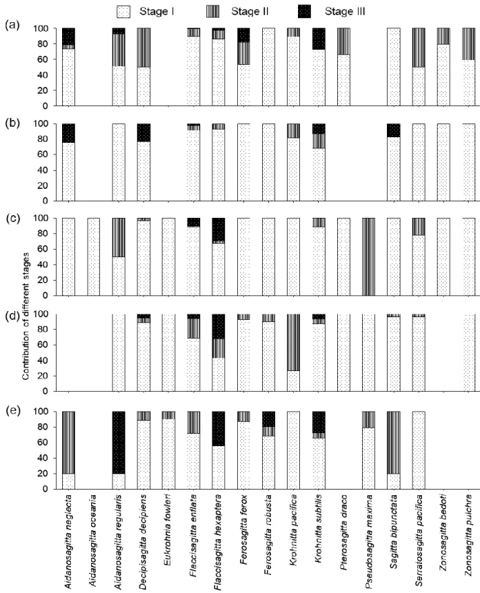
The constrained Redundancy analysis (RDA) was used as in multivariate space it best explains 157
the linear relationships between response and explanatory variables (Van den Wollenberg 1977).
158
The advantage of RDA is that it displays a simultaneous representation of the observations of the 159
response variables (Chaetognatha) and explanatory variables (physical and chemical variables 160
and Copepoda), and the position of the variables in the tri-plot helps visualizing their 161
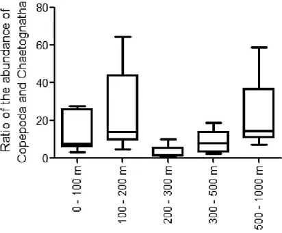
relationships.
162 163
Results 164
Physical and chemical environment 165
8
Sea surface temperatures (at 3 m depth) varied between 23.1 and 28.5°C (average ± SD, 26 ± 1.8 166
°C) and decreased towards the north (Fig. 2a). In the vertical temperature profile, a strong 167
gradient was observed in the upper 200 m of the water column and more pronounced in the south 168
(Fig. 2a). Sea surface salinity also showed a latitudinal gradient with a marked increase towards 169
the north (range 37.3 − 40.4; average 39 ± 1.1) (Fig. 2b). The stratification in the vertical salinity 170
profile was evident in the upper 200 m with stronger gradient towards the south (Fig. 2b). Spatial 171
variation in the surface DO was marginal (average 253.9 ± 19.2 µmol kg -1), with a sharp 172
gradient in the vertical profile below 50 m (Fig. 2c). Low DO (<100 µmol kg -1) at depths were 173
evident throughout the study region. In the south, the oxygen minimum layer was observed 174
between 150 – 800 m whereas in the north it was between 400 – 650 m (Fig. 2c).
175
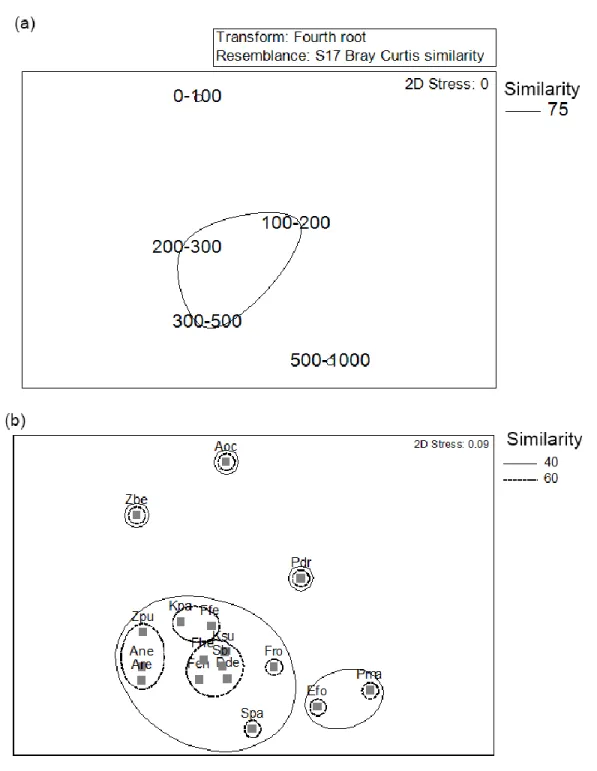
Copepoda abundance 176
The upper 100 m contributed 79.3% to the total copepod abundance over the entire 1000 m water 177
column. Copepoda abundances in this layer varied between 37.9 and 74.9 ind m-3 with an 178
average abundance of 53.4 ± 14.3 ind m-3 (Supplementary Fig. 1). The variation in the 179
abundance along different depth zones was significantly different (one-way ANOVA, F4,25 = 180
67.63, P < 0.001). While there was a pronounced decrease from the 0 – 100 m stratum to the 100 181
– 200 m stratum, the further decrease in abundance was not consistent with increasing depth 182
(Supplementary Fig. 1a). The abundance was observed to be lowest at the 200 – 300 m depth at 183
all sampling sites except off Farasan where it was lowest at 300 – 500 m (Supplementary Fig. 1).
184
Chaetognath abundance, community structure and vertical distribution 185
Similar to the copepod community, Chaetognatha were most numerous in the upper 100 m 186
contributing to 74.2% to their total population over the entire sampling depths (Supplementary 187
Fig. 1). The variation in the Chaetognatha abundance over depths were statistically significant 188
9
(one-way ANOVA, F4,25 = 10.84, P < 0.001). The Chaetognatha abundances sharply decreased 189
below 100 m at most sites and abundances showed an intermediate low at 100 – 200 m depth 190
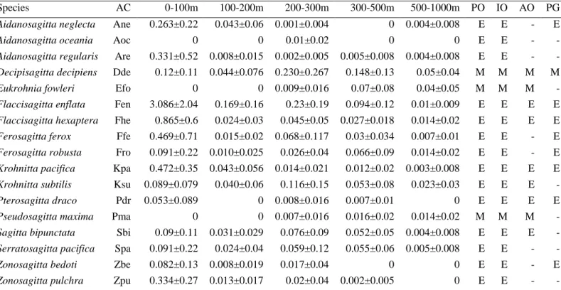
before reaching 500 – 1000 m (Supplementary Fig. 1). A total of 17 species belonging to 11 191
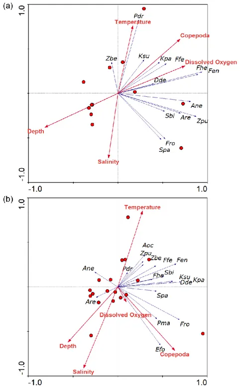
genera were observed (Table 1). Although Chaetognatha abundance was higher in the upper 100 192
m, a maximum number of species was recorded from 200 – 300 m (17) and a minimum at 100 – 193
200 m and 500 – 1000 m (12 each, respectively). Flaccisagiita enflata was the dominant species 194
in the upper two depth strata, whereas Decipisagitta decipiens dominated depths below 500 m 195
(Fig. 3). Nine species (Krohnitta pacifica, Krohnitta subtilis, Aidanosagitta regularis, 196
Decipisagitta decipiens, Flaccisagitta enflata, Flaccisagitta hexaptera, Ferosagitta ferox, 197
Sagitta bipunctata, and Zonosagitta pulchra) were observed at all stations in one or more depth 198
strata despite different abundances. Among the epipelagic Chaetognatha, nine species were 199
observed in the entire 1000 m, and five of them had >75% of their abundance in the upper 100 m 200
(Table 1 and Supplementary Fig. 2). The epipelagic Pterosagitta draco and Zonosagitta pulchra 201
were observed in the upper 500 m, and showed higher abundances in the upper 100 m (>75%), 202
whereas the distribution of Zonosagitta bedoti was restricted to the upper 300 m (Table 1). Of 203
the mesopelagic species, only Decipisagitta decipiens was present throughout the 1000 m and 204
had higher abundances at 200 – 500 m. Eukrohnia fowleri and Pseudosagitta maxima were 205
observed only below 200 m especially with high preferences for waters below 300 m (Table 1).
206
Although the weighted mean depth (Zm) of the chaetognaths varied among species, it was less 207
than 100 m depth for majority of the epipelagic species (Fig. 4). The Zm of the mesopelagic 208
species ranged between 352 and 556 m (Fig. 4). Spatially, the occurence of the majority of the 209
epipelagic species in the deeper layers was higher in Duba, the northernmost station 210
(Supplementary Table 2). Based on the maturity stages of the species of chaetognaths, the 211
10
immature individuals dominated at most depths (Fig. 5). Both maturing and mature individuals 212
of the majority of the epipelagic species had a preference for surface waters (0 – 100 m) (Fig. 5) 213
Chaetognatha-Copepoda interrelationship 214
A positive relation was observed between the abundances of Copepoda and Chaetognatha 215
(Pearson correlation; R = 0.761, P < 0.01). The ratio of the abundance of the Copepoda and 216
Chaetognatha varied among the depth layers (Fig. 6). It was relatively higher in the upper two 217
layers and in the deeper 500 – 1000 m depth, but lower in the mid-depth waters (median 7.8, 218
13.9, 1.7, 8, and 14.3, in 0 – 100 m, 100 – 200 m, 200 – 300 m, 300 – 500 m and 500 – 1000 m 219
depth, respectively).
220
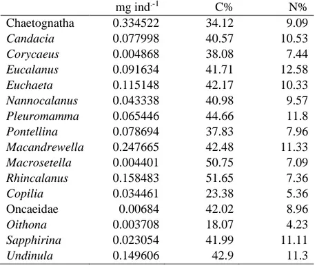
Table 2 displays the C and N content of Chaetognatha and of the dominant genus of the 221
Copepoda. The C and N of Chaetognatha was 34.12 and 9.09% of their dry weight, respectively.
222
In Copepoda, the percentage of C varied between 18.07% to 51.65% of their dry weight, and in 223
case of N it ranged between 4.23% and 12.58% among the different genera. To approximate the 224
C and N content of the total Copepoda community, an average C and N content of the dominant 225
Copepoda genera were used for the remaining Copepoda community. Considering the total 226
volume of the upper 100 m of the Red Sea as 3.433 ×10¹³ m-3, Chaetognatha contained ~25,222 t 227
C and 3,719 t N, respectively. In case of Copepoda, the elemental content was 95451 t and 21865 228
t for C and N, respectively. The total amount of C in the Chaetognatha was 26.4% of the total C 229
content of Copepoda and in case of N content this value was 30.7%. The relative trophic position 230
for the Chaetognatha community was 3.2 ± 0.4 (min 2.7 max 4.1; n = 31 samples, a composite of 231
514 specimens, Kürten et al. 2016).
232
The NMDS plot based on the abundance of Chaetognatha species along the depth layers, 233
exhibited a discrete ordination of the upper 0 – 100 m and deeper 500 – 1000 m from the other 234
11
depth zones with a Kruskal stress value of 0 (Fig. 7a). The overlay cluster based on the 75%
235
similarity level revealed a group of the mid-depth zones together (100 – 200 m, 200 – 300 m, and 236
300 – 500 m) (Fig. 7a). The NMDS plotted to evaluate the similarity in the distribution of the 237
Chaetognatha species revealed a large group with majority of the epipelagic species and another 238
group with two mesopelagic species based on the 40% similarity (Fig. 7b).
239
α and β-diversity 240
The species diversity (H´) varied both spatially and temporally and based on the depth-wise 241
average value it was maximum at 200 – 300 m (average 2.29 ± 0.45, 2.3 ± 0.88, 2.64 ± 0.49, 242
2.61 ± 0.54, and 2.22 ± 0.6, in 0 – 100 m, 100 – 200 m, 200 – 300 m, 300 – 500 m, and 500 – 243
1000 m, respectively). The relative variability of the Chaetognatha assemblages within each 244
stations (i.e. intragroup β-dissimilarity) exhibited the lowest value off Duba (Supplementary 245
Table 3, based on the MVDISP analysis). The pairwise inter-station β-dissimilarity based on the 246
index of multivariate dispersion (IMD) showed varying results among sites (Supplementary 247
Table 3). In general, the southernmost two stations had high IMD values with most of the other 248
sampling locations (Supplementary Table 3). The northernmost station had a high dissimilarity 249
with its nearby station Mabahiss (0.62).
250
Redundancy analysis (RDA) 251
The RDA triplots indicated the preferred environment of the Chaetognatha species. Most of the 252
epipelagic Chaetognatha were positively correlated with DO and the abundance of their 253
dominant prey Copepoda (Fig. 8a). The abundances of mesopelagic Eukrohnia fowleri and 254
Pseudosagitta maxima also exhibited a similar result having positive relation with the abundance 255
of Copepoda and DO (Fig. 8b).
256 257
12 Discussion
258
The ecohydrographic framework of the Red Sea helped to understand the complexity in the 259
biotic-abiotic relationships of the Chaetognatha community. The lower salinity in the upper 100 260
m, chiefly up to 19°N, relates to the inflow of GAW into the Red Sea and corroborates earlier 261
observations and modeling studies (Stubbings 1939; Maillard and Soliman 1986; Sofianos and 262
Johns 2007). Theoverturning circulation in the northern Red Sea is another important factor that 263
governs the hydrography of this basin. The outcome of this overturning circulation is the sinking 264
of surface waters in the north which was clearly evident in the salinity structure around 27°N 265
(Fig. 2b). The winter surface cooling leads to deep convection in the northern Red Sea and 266
results in a near-homogeneous water up to subsurface layers (Kürten et al. 2016; Fig. 2).
267
However, the sinking of the isothermal lines at the northernmost location supports the salinity 268
based observation of the sinking of water to deeper layers.
269
The variability in the physical and chemical characteristics in the Red Sea influenced the 270
plankton distribution. In the upper 100 m water, the Chaetognatha abundance was high in 271
Atlantis II and off Duba. At the Atlantis II, upwelling of nutrient-rich water contributed to the 272
conspicuous preponderance of diatoms (Kürten et al. 2016). It is suggested that the higher 273
availability of diatoms supported increased abundances of Copepoda and in turn sustained higher 274
Chaetognatha abundance in this location. Similarly, the increased abundance of diatoms off 275
Duba also offered sufficient food for zooplankton as indicated by increased chlorophyll a and 276
particulate organic nitrogen as proxies for phytoplankton biomass (Kürten et al. 2016).
277
The existence of hypoxic waters helps explaining the sudden drop in the Chaetognatha abundance 278
below 100 m. Chaetognatha are sensitive to low DO, as was shown, for example, in the adjacent 279
Arabian Sea where Chaetognatha are scarce in oxygen deficient zones (Kusum et al. 2011). Hence, 280
13
the sharp gradients in DO leading to hypoxia in the 100 – 200 m in the Red Sea are likely to lower 281
Chaetognatha abundances at this depth. The Zm of majority of the epipelagic species was less than 282
100 m indicating their preference to the upper oxygenated water. The Zs varied among the species 283
and the relatively lower Zs in epipelagic species like Zonosagitta bedoti and Zonosagitta pulchra 284
points out their restricted vertical distribution (Fig. 4). The marked positive relation between the 285
abundance of most of the Chaetognatha species and DO corroborates the vital role of DO in 286
structuring the Chaetognatha population (Fig. 8), a relationship typical for plankton distribution in 287
the oxygen minimum zones around the world (Wishner et al. 1995).
288
The higher abundance of the epipelagic Chaetognatha inhabiting the oxygenated upper 100 289
m was reflected in the separation of this depth stratum from the aphotic zone (Fig. 7a). Among the 290
nine epipelagic Chaetognatha observed, five species had >75% of their abundance in the upper 291
100 m, which points towards their preferences for relatively well-oxygenated surface waters. The 292
group of the majority of the epipelagic Chaetognatha species in the NMDS plot (Fig. 7b) 293
corroborated their preferences for the similar environments. The higher abundance of Copepoda, 294
their primary prey at this depth, might have also favored their higher sustenance and abundances.
295
Although gut content analysis of the Chaetognatha was not carried out in the present study, 296
Copepoda are typically the most preferred prey of Chaetognatha (Kehayias 2003; Giesecke and 297
González 2004; Terazaki 2004; Yoon et al. 2016). The marked positive correlation between prey 298
and predators confirms the important trophic link. In the RDA analysis, the observed positive 299
association of the majority of the epipelagic and mesopelagic species of Chaetognatha with the 300
abundance of Copepoda (Fig. 8) further validates their trophic relations. The relative trophic 301
position for the Chaetognatha community in this study was 3.2 ± 0.4 where producer species were 302
assigned to trophic level 1, and the consumer values range from 2 (primary consumers) to 5 or 303
14
greater. This relative trophic position exhibits their importance as the secondary consumer in the 304
pelagic ecosystem. The feeding rate of the Chaetognatha has been found to vary among tropical, 305
temperate, and polar organisms (Oresland 2000; Giesecke and González 2012). Flaccisagitta 306
enflata, the dominant Chaetognatha in the upper 300 m is capable of consuming up to 10 – 12 prey 307
items day-1, whilst its feeding rate depends on prey availability (Reeve 1980; Kimmerer 1984).
308
The higher values of the ratio of the abundance of the Copepoda and Chaetognatha (median 7.8, 309
and 13.9, in 0 – 100 m, and 100 – 200 m, respectively) indicates a favorable environment for the 310
Chaetognatha. The lower ratios in the mid-depth waters (median 1.7, and 8, in 200 – 300 m, 300 311
– 500 m, respectively) indicates a food-limited environment for the Chaetognatha compared to the 312
upper layers. This scenario differs from the northern Arabian Sea, where the prey – predator ratio 313
was higher in the acute oxygen depleted mid-depth waters than in surface waters (Kusum et al.
314
2011).
315
The abundance of both Copepoda and Chaetognatha in the upper 100 m was > 70% of 316
their total population in the entire 1000 m water column and hence based on the information in 317
the available literature we estimated the predation pressure of the Chaetognatha on the Copepoda 318
in this stratum. We considered the predation impact (the percentage of the copepod standing 319
stock consumed per day) of the dominant species F. enflata and also of the total Chaetognatha 320
community. To calculate the predation impact, the prey day-1 for each individual of 321
Chaetognatha was estimated based on the result observed in the upper 100 m by Kehiyas (2003, 322
Tables 4 and 5) in the Mediterranean Sea (F. enflata: ave 0.96 ± 0.58, range 0.46 – 1.8 prey per 323
day; Total Chaetognatha: ave 1.36 ± 1.16, range 0.64 – 3.9 prey per day). The Mediterranean Sea 324
has many ecohydrographic similarities with the Red Sea, e.g. high salinity, low productivity, and 325
zooplankton stock (Gotsis-Skretas et al. 1999). The predation impact of F. enflata varied 326
15
between 1.51 and 11.7 (av. 5.8 ± 4) with an increasing trend towards the north (Supplementary 327
Table 4). The average (±SD) predation impact was higher than in the Cretan Passage (1.3 ± 0.5) 328
and Rhodes Sea (4.8 ± 1.4), but lower than the Ionian Sea (28.5 ± 2.8) and the Cretan Sea (21.7 ± 329
6) in the Mediterranean. The predation impact of the total Chaetognatha community (13 ± 9.8, 330
range 3.6 - 30.6) showed a similar trend to that of the F. enflata and clearly indicates the 331
significance of this plankton taxon in the trophic energy transfer.
332
Interestingly, in the upper 100 m, the C and N contents of the Chaetognatha community 333
were 26.4% and 30.7%, of the Copepoda community, which were higher than the estimated 334
predation impact of the total Chaetognatha on the Copepoda (13 ± 9.8). Compared to the 335
copepods, the relatively larger size of the individuals of Chaetognatha as seen also in the high 336
dry mass per individual (Table 2), might have resulted in asymmetry between the ratio of the 337
elemental composition and the predation pressure of Chaetognatha on the Copepoda.
338
In the subsurface and deeper waters, the Chaetognatha populations of the three mid-depth 339
zones between 100 – 500 m were closely ordinated in the NMDS plot (Fig. 7), most likely 340
attributable to the hypoxic conditions at the mid-depths strata. Similar to the observation in the 341
Arabian Sea, the hypoxic waters exerted a profound impact on the vertical distribution of the 342
Chaetognatha community of the Red Sea, but species like Sagitta bipunctata and Serratosagitta 343
pacifica which were found to be mostly restricted to upper waters in the northern Arabian Sea 344
(Kusum et al. 2011), were present in most of the depth zones of the Red Sea. Unlike the northern 345
Arabian Sea, the absence of the acute oxygen depleted waters (DO <9 µmol kg -1) in the mid- 346
depth zones of the study region might have permitted these species to inhabit these waters.
347
The intrusion of GAW plays a role in the spatial variability of the Chaetognatha community in the 348
Red Sea, similar to other plankton taxa, e.g. Foraminifera (Siccha et al. 2009). The upper 150 m 349
16
of the southernmost two stations were characterized by relatively low saline, warm, and 350
oxygenated waters which indicated the inflow of GAW into the Red Sea. The importance of the 351
inflow of GAW for the spatial distribution in the Red Sea was also reflected in the high IMD at 352
the two stations in the south with the other sampling locations (Supplementary Table 3). The 353
intragroup β-dissimilarity was also higher in these southernmost stations. The presence of both 354
low saline waters from the Gulf of Aden in the surface and conversely high saline Red Sea Deep 355
Water at depths may contribute to intra-station community dissimilarity at these two stations 356
compared to other locations where salinity was higher (>40). Earlier Casanova (1985) reported 357
Zonosagitta bedoti as an indicator of the surface inflow of GAW. The limitation of this species’
358
presence to the southern stations up to 18° N supports this view. In contrast to previous 359
observations which documented the presence of Pterosagitta draco mostly in the southern part of 360
the Red Sea (Casanova 1986), P. draco was found also in the northern part of the Red Sea in the 361
present study. This implies that the northward advection of GAW influences the distribution of 362
this species farther than expected. This observation also refutes the view of Halim (1969), who 363
noted that the seasonal and geographic distribution of Chaetognatha affords no evidence of 364
dependence on the southern inflow.
365
In the Red Sea, the gradual increase in salinity from south to north is known to set ecophysiological 366
boundaries for faunal assemblage along the basin's axis, e.g. Foraminifera (Fenton et al. 2000;
367
Siccha et al. 2009). Additionally, the wind jet near the Tokar Gap at 19°N also plays a role in the 368
ecohydrographic division in the Red Sea as it influences the regional circulation (Stubbings 1939;
369
Zhai and Bower 2013; Abdullah et al. 2018). Although, these factors contributed to the β- 370
dissimilarity between the locations of the north and south, the majority of species were observed 371
17
at most of the sampling locations in varying abundances. These Indo-Pacific species, due to their 372
euryhaline nature, might have survived in this ocean basin.
373
Another interesting feature that modulated the vertical distribution of the Chaetognatha 374
community was the convective mixing in the northern Red Sea. The downward inclination of the 375
isolines of salinity, temperature and DO at the northernmost station Duba (Fig. 2) corroborates 376
this notion. Association of Chaetognatha with upwelled or downwelled water has been 377
documented before ascertaining their role as indicators of physical processes (Thiriot 1978;
378
Kusum et al. 2014; Nair et al. 2015; Al-Aidaroos et al. 2016). Here, the sinking of water masses 379
associated with the deep water formation in the northern Red Sea is a plausible explanation for 380
higher epipelagic Chaetognatha abundances in deeper layers (Supplementary Table 2).
381
A total of 17 Chaetognatha species were observed during the present study in the Red 382
Sea. The observed species are all common in the northern Indian Ocean and many of them have 383
Indo-Pacific affinity and are absent from the Atlantic Ocean (Table 1). The importance of 384
Flaccisagitta enflata and Decipisagitta decipens, the dominant species of the upper 300 m and 385
300 – 500 m strata, respectively, concurs with the observation in the northern Indian Ocean (Nair 386
et al. 2015) and suggests similarity in Chaetognatha community structure between these two 387
tropical ecoregions. But, the mesopelagic Eukrohnia fowleri and Pseudosagitta maxima, which 388
often dominate the Chaetognatha community in the 500 – 1000 m depth of the northern Indian 389
Ocean (Kusum et al. 2014), were less numerous. The shallow sill of the Bab-al-Mandab (160 m) 390
connecting the Red Sea and the Arabian Sea is considered to limit the presence of the deeper 391
water species in the Red Sea (Casanova 1986). Nevertheless, the occurrence of mesopelagic 392
species in the upper waters in association with upwelling has been reported before (Kusum et al.
393
2014, Nair et al. 2015). This process offers a plausible explanation for their presence in the Red 394
18
Sea. In fact, the bathypelagic Chaetognatha in the Arabian Sea like Eukrohnia hamata, E. minuta 395
and E. bathypelagica were absent in the Red Sea, indicating the restriction imposed by the 396
shallow sill on their distribution. The scenario of the restricted abundance of mesopelagic species 397
and absence of bathypelagic species in the Mediterranean Sea (Casanova 1986), which is also 398
connected through a shallow sill to the Atlantic Ocean supports that such barriers are important 399
to understand the distribution of the Chaetognatha.
400
The number of species recorded from the 1000 m of Red Sea was relatively low 401
compared to the northern Indian Ocean or the Pacific Ocean (Nair 1978; Pierrot-Bults and Nair 402
1991). The less variability in the physical variables in this basin compared to that of Indian 403
Ocean or Pacific Ocean might be the reason for the low diversity in the Chaetognatha 404
community of the Red Sea. Similarly, the lower diversity of Chaetognatha in the Persian Gulf 405
(total 12, Furnestin and Codaccioni 1968; Haghi et al. 2010), another hyperhaline semi-enclosed 406
inlet of the Indian Ocean, further supports the view.
407
The patterns in vertical abundance and the species diversity distribution seem 408
contradictory as both number of species and the species diversity index reached their maximum 409
not at 0 – 100 m depth, but at 200 – 300 m. The higher abundance in the euphotic zone was 410
mainly attributable to epipelagic species, whereas the abundance at 200 – 300 m was the result of 411
mixed populations of both epipelagic and mesopelagic Chaetognatha species (Table 1), leading 412
to a higher species diversity at this depth compared to the surface waters. This subsurface 413
diversity maximum of Chaetognatha was in accordance with the earlier observation in the Indian 414
Ocean (Nair 1978; Kusum et al. 2011), as well as with those of Copepoda in the Pacific Ocean 415
(Saltzman and Wishner 1997).
416
19
The varied physiology and the ecohydrographic interrelations of the different maturity 417
stages of the plankton community can be the discernible factors affecting their vertical 418
distributions in the water column (Capitanio and Esnal 1998). The dominance of the immature 419
population throughout the water column observed in the study was consistent with the earlier 420
observation in the surface water from this basin (Al-Aidaroos et al. 2017). The question if mature 421
stages of Chaetognatha are more sensitive to oxygen deficient waters compared to immature 422
stages was also assessed in the present study. Among the five depth layers, the relatively higher 423
abundances of maturing and matured individuals of epipelagic species in the well-oxygenated 424
upper layer may corroborate the notion that mature organisms, due to their higher oxygen 425
demands for egg and sperm production (Wishner et al. 2000) avoid the hypoxic mesopelagic 426
zones and therefore congregate the upper and deeper waters with higher DO.
427
In brief, the macroecology of the Chaetognatha community of the Red Sea was governed 428
by a multitude of indigenous characteristics of this unique ocean basin. The distinct water mass 429
characteristics of GAW, characterized by low salinity, high CDOM and low DO concentration 430
(Zarokanellos and Jones 2018), exerted an important role in structuring the Chaetognatha 431
community. The presence of Zonosagitta bedoti, for instance, can be viewed as an indicator of 432
the surface inflow of GAW as described by Casanova (1985). The evident high β-dissimilarity 433
between the Chaetognatha community of the southern regions and other sampling locations 434
corroborate the importance of GAW intrusions. The overturning circulation and the sinking of 435
water mass in the north is another physical characteristic of the Red Sea which influenced the 436
vertical distribution of the Chaetognatha community. In addition to this, hypoxic waters in the 437
mid-depth zones of the Red Sea had an important role in the vertical distribution of 438
Chaetognatha. The results of the predation impact and the elemental analysis of Copepoda and 439
20
Chaetognatha confirmed the important trophic link between these two prey-predator taxa. The 440
present study providing detailed information on the ecohydrographic drivers that govern the 441
distribution and community structure of a major plankton component of the Red Sea will be 442
important to unravel the macro ecology of this topographically unique but ecologically 443
significant ocean basin in the world ocean.
444
Acknowledgements and Funding 445
This project was funded by the Deanship of Scientific Research (DSR) at King Abdulaziz 446
University, Jeddah, under grant no. RG-1-150-35. The authors, therefore, acknowledge with 447
thanks DSR technical and financial support. We further extend our gratitude towards the 448
Helmholtz-Center for Ocean Research GEOMAR for the successful collaboration (Jeddah 449
Transect Project) with the King Abdulaziz University. The authors also thank the Master and 450
crew of RV Pelagia (cruise 64PE351) for their help in the field. During the writing phase of this 451
manuscript, BK was supported through baseline funds of BHJ (KAUST).
452
Compliance with ethical standards 453
Conflict of interest The authors declare that they have no conflict of interest.
454
Ethical approval 455
All applicable international, national and/or institutional guidelines for the care and use of 456
animals were followed.
457 458
459 460 461 462 463
21 References
464
Abdulla CP, Alsaafani MA, Alraddadi TM. Albarakati AM (2018) Mixed layer depth variability 465
in the Red Sea. Ocean Sci 14:563-573.
466
Al-Aidaroos AM, Salama AJ, El-Sherbiny MM (2016) New record and redescription of 467
Calanopia thompsoni A. Scott, 1909 (Copepoda, Calanoida, Pontellidae) from the Red 468
Sea, with notes on the taxonomic status of C. parathompsoni Gaudy, 1969 and a key to 469
species. ZooKeys 552:17-32. doi:10.3897/zookeys.552.6180.
470
Al-Aidaroos AM, Karati KK, El-Sherbiny MM, Devassy RP, Kürten B (2017) Latitudinal 471
environmental gradients and diel variability influence abundance and community 472
structure of Chaetognatha in Red Sea coral reefs. Syst Biodivers 15:35-48.
473
Alvariño A (1964). Bathymetric distribution of chaetognaths. Pac Sci 18:64-82.
474
Anderson MJ, Crist TO, Chase, JM, Vellend M, Inouye BD, Freestone AL, Sanders NJ, Cornell 475
HV, Comita LS, Davies KF, Harrison SP (2011) Navigating the multiple meanings of β 476
diversity: a roadmap for the practicing ecologist. Ecol Lett 14:19-28.
477
Bohata K, Koppelmann R (2013) Chaetognatha of the Namibian upwelling region: taxonomy, 478
distribution and trophic position. PloS one, 8:e53839.
479
Buchanan PJ, Beckley LE (2016) Chaetognatha of the Leeuwin Current system: oceanographic 480
conditions drive epi-pelagic zoogeography in the south-east Indian Ocean. Hydrobiologia 481
763:81-96.
482
Capitanio FL, Esnal GB (1998) Vertical distribution of maturity stages of Oikopleura dioica 483
(Tunicata, Appendicularia) in the frontal system off Valdés Peninsula, Argentina. B Mar 484
Sci 63:531-539.
485
22
Casanova JP (1985) Les Chaetognathes de la Mer Rouge. Rapp. P.-v. Reun Commn Int Explor 486
Scient Mer Mediterr 29:269274.
487
Casanova JP (1986) Similarity of plankton distribution patterns in two nearly land-locked seas:
488
the Mediterranean and the Red Sea. In: Pierrot-Bults AC, van der Spoel S, Zahuranec BJ, 489
Johnson RK (Eds.) UNESCO technical paper in Marine Science, 49:42-46.
490
Clarke KR, Gorley RN (2006) PRIMER v6: User Manual/Tutorial. Plymouth, UK: PRIMER-E 491
Ltd.
492
Devassy RP, El-Sherbiny MM, Al-Sofyani AM, Al-Aidaroos AM (2017) Spatial variation in the 493
phytoplankton standing stock and diversity in relation to the prevailing environmental 494
conditions along the Saudi Arabian coast of the northern Red Sea. Mar Biodivers 47:995- 495
1008.
496
Ducret F (1973). Contribution à l'étude des chaetognathes de la Mer Rouge. Beaufortia 20: 135- 497
153.
498
Echelman T, Fishelson L (1990) Surface zooplankton dynamics and community structure in the 499
Gulf of Aqaba (Eilat), Red Sea. Mar Biol 107:179-190.
500
El-Sherbiny MM, Hanafy MH, Aamer MA (2007) Monthly Variations in Abundance and 501
Species Composition of the Epipelagic Zooplankton off Sharm El-Sheikh, Northern Red 502
Sea. Res J Environ Sci 1:200-210.
503
El-Sherbiny MM, Al-Aidaroos AM (2017) A new species of Calanopia (Copepoda, Calanoida, 504
Pontellidae) from the plankton of the central Red Sea. Mar Biodivers 47:1137-1145.
505
Fenton M, Geiselhart S, Rohling EJ, Hemleben C (2000) Aplanktonic zones in the Red Sea. Mar 506
Micropaleontol 40:277-294.
507
23
Furnestin ML, Codaccioni JC (1968) Chaetognathes du Nord-Ouest de l'Océan Indien (golfe 508
d'Aden, Mer d'Arabie, golfe d'Oman, golfe Persique). Cah ORSTOM Sér Océanogr 509
6:143-171.
510
Giesecke R, González HE (2004) Feeding of Sagitta enflata and vertical distribution of 511
Chaetognatha in relation to low oxygen concentrations. J Plankton Res 26:475-486.
512
Giesecke R, González HE (2012) Distribution and feeding of chaetognaths in the epipelagic zone 513
of the Lazarev Sea (Antarctica) during austral summer. Polar Biol 35:689-703.
514
Gotsis-Skretas O, Pagou K, Moraitou-Apostolopoulou M, Ignatiades L (1999) Seasonal 515
horizontal and vertical variability in primary production and standing stocks of 516
phytoplankton and zooplankton in the Cretan Sea and the Straits of the Cretan Arc 517
(March 1994–January 1995). Prog Oceanogr 44:625-649.
518
Grasshoff K (1969) Zur Chemie des Roten Meeres und des Inneren Golfs von Aden nach 519
Beobachtungen von FS "Meteor" während der Indischen Ozean Expedition 1964/65 520
Meteor Forschungsergebnisse, Deutsche Forschungsgemeinschaft, Reihe A Allgemeines, 521
Physik und Chemie des Meeres. Gebrüder Bornträger, Berlin, Stuttgart, pp 1-76.
522
Haghi M, Savari A, Madiseh SD, Zakeri M (2010) Abundance of pelagic chaetognaths in 523
northwestern Persian Gulf. Plankton Benthos Res 5:44-48.
524
Halim Y (1984) Plankton of the Red Sea and the Arabian Gulf. Deep Sea Res I 31:969-982.
525
Harris R, Wiebe P, Lenz J, Skjoldal HR, Huntley ME (eds) 2000. ICES Zooplankton 526
Methodology Manual. Academic Press, London.
527
Kehayias G (2003) Quantitative aspects of feeding of chaetognaths in the eastern Mediterranean 528
pelagic waters. J Mar Biol Ass UK 83:559-569.
529
24
Kimmerer WJ (1984) Selective predation and its impact on prey of Sagitta enflata 530
(Chaetognatha). Mar Ecol Prog Ser 15:55-62.
531
Kürten B, Khomayis HS, Devassy R, Audritz S, Sommer U, Struck U, El‐ Sherbiny MM, Al- 532
Aidaroos AM (2014) Ecohydrographic constraints on biodiversity and distribution of 533
phytoplankton and zooplankton in coral reefs of the Red Sea, Saudi Arabia. Mar Ecol 534
36:1195-1214.
535
Kürten B, Khomayis HS, Devassy R, Audritz S, Sommer U, Struck U, El-Sherbiny MM, Al- 536
Aidaroos AM (2015) Ecohydrographic constraints on biodiversity and distribution of 537
phytoplankton and zooplankton in coral reefs of the Red Sea, Saudi Arabia. Mar Ecol 538
36:1195-1214.
539
Kürten B, Al-Aidaroos AM, Kürten S, El-Sherbiny MM, Devassy RP, Struck U, Zarokanellos N, 540
Jones BH, Hansen T, Bruss G, Sommer U (2016) Carbon and nitrogen stable isotope 541
ratios of pelagic zooplankton elucidate ecohydrographic features in the oligotrophic Red 542
Sea. Prog Oceanogr 140:69-90.
543
Kusum KK, Vineetha G, Raveendran TV, Muraleedharan KR, Nair M, Achuthankutty CT 544
(2011) Impact of oxygen-depleted water on the vertical distribution of Chaetognatha in 545
the northeastern Arabian Sea. Deep Sea Res Part I 58:1163-1174.
546
Kusum KK, Vineetha G, Raveendran TV, Muraleedharan KR, Biju A, Achuthankutty CT (2014) 547
Influence of upwelling on distribution of Chaetognatha (zooplankton) in the oxygen 548
deficient zone of the eastern Arabian Sea. Cont Shelf Res 78:16-28.
549
Lima ME (2014) Characterization of zooplankton communities associated with an anticyclonic 550
Eddy in the northeast of the islands of Cabo Verde. Doctoral dissertation, Universidade 551
de Cabo Verde.
552
25
Maillard C, Soliman G (1986) Hydrography of the Red-Sea and exchanges with the Indian- 553
Ocean in summer. Oceanol Acta 9:249-269.
554
McLaren IA (1969). Population and production ecology of zooplankton in Ogac Lake, a 555
landlocked fiord on Baffin Island. J Fish Res Board Canada 26:1485-1559.
556
Miller AR (1964) Highest salinity in the world ocean. Nature 203:590-591.
557
Nagai N, Tadokoro K, Kuroda K, Sugimoto T (2006) Occurrence characteristics of 558
Chaetognatha species along the PM transect in the Japan Sea during 1972–2002. J 559
Oceanogr 62:597-606.
560
Nair VR (1978) Bathymetric distribution of Chaetognatha in the Indian Ocean. Indian J Mar Sci 561
7:276–82.
562
Nair VR (2003) Digitized inventory of marine bioresources. Chaetognatha. National Institute of 563
Oceanography. www.nio.org/index/option/comnomenu/task/show/tid/2/sid/18/id/6 564
Nair VR, Kusum KK, Gireesh R, Nair M (2015) The distribution of the Chaetognatha population 565
and its interaction with environmental characteristics in the Bay of Bengal and the 566
Arabian Sea. Mar Biol Res 11:269-282.
567
Øresland V (2000) Diel feeding of the chaetognath Sagitta enflata in the Zanzibar Channel, 568
western Indian Ocean. Mar Ecol Prog Ser 193:117-123.
569
Pierrot-Bults AC, Nair VR (1991) Distribution patterns in Chaetognatha. In: Bone Q, Kapp H, 570
Pierrot-Bults AC (Eds.) The Biology of Chaetognatha. Oxford University, pp 86-116.
571
Reeve MR (1980) Comparative experimental studies on the feeding of chaetognaths and 572
ctenophores. J Plank Res 2:381-393.
573
Saltzman J, Wishner KF (1997) Zooplankton ecology in the eastern tropical Pacific oxygen 574
minimum zone above a sea- mount: 1. General trends. Deep-Sea Res I 44:907–930.
575
26
Siccha M, Trommer G, Schulz H, Christoph H, Kucera M (2009) Factors controlling the 576
distribution of planktonic foraminifera in the Red Sea and implications for the 577
development of transfer functions. Mar Micropaleontol 72:146-156.
578
Sofianos SS, Johns WE (2002) An oceanic general circulation model (OGCM) investigation of 579
the Red Sea circulation, 1. Exchange between the Red Sea and the Indian Ocean. J 580
Geophys Res: Oceans, 107(C11).
581
Sofianos SS, Johns WE (2003) An oceanic general circulation model (OGCM) investigation of 582
the Red Sea circulation: 2. Three‐ dimensional circulation in the Red Sea. J Geophys 583
Res: Oceans, 108(C3).
584
Sofianos SS, Johns WE (2007), Observations of the summer Red Sea circulation, J Geophys Res 585
112(C6), C06025, doi:10.1029/2006jc003886.
586
Stubbings HG (1939) The marine deposits of the Arabian Sea: an investigation into their 587
distribution and biology. Trustees of the British Museum, London.
588
Terazaki M (2013) Feeding of Carnivorous Zooplankton, Chaetognatha. Dynamics and 589
Characterization of Marine Organic Matter, 2, p.257.
590
Thiriot A (1978) Zooplankton communities in the west African upwelling area. In: Boje R, 591
Tomczak M (Eds.) Upwelling ecosystems. Springer-Verlag, Berlin, p32-61.
592
Vanden Wollenberg AL. (1977). Redundancy analysis. An alternative for canonical correlation 593
analysis. Psychometrika 42:207–219.
594
Warwick RM, Clarke KR (1993) Taxonomic distinctness and environmental assessment. J Appl 595
Ecol 35, 532e543.
596
Wiebe PH, Allison D, Kennedy M, Moncoiffé G (2014) A vocabulary for the configuration of 597
net tows for collecting plankton and micronekton. J Plank Res 37: 21-27 598
27
Wishner KF, Ashjian CJ, Gelfman C, Gowing MM, Kann L, Levin LA, Mullineaux LS, 599
Saltzman J (1995) Pelagic and benthic ecology of the Eastern Tropical Pacific oxygen 600
minimum zone. Deep-Sea Res I 42:93-115.
601
Wishner KF, Gowing MM, Gelfman C (2000) Living in suboxia: ecology of an Arabian Sea 602
oxygen minimum zone copepod. Limnol Oceanogr 45:1576–1593.
603
Yoon H, Ko AR, Kang JH, Choi JK, Ju SJ (2016) Diet of Chaetognatha Sagitta crassa and S.
604
nagae in the Yellow Sea Inferred from Gut Content and Fatty Acid Analyses. Ocean 605
Polar Res 38:5-46.
606
Zarokanellos ND, Jones BH (2018) Winter mixing, mesoscale eddies and eastern boundary 607
current: Engines for biogeochemical variability of the central Red Sea during winter/early 608
spring period. Biogeosciences Discuss 2018: 1-44 doi 10.5194/bg-2017-544.
609
Zhai P, Bower A (2013) The response of the Red Sea to a strong wind jet near the Tokar Gap in 610
summer. J Geophys Res Oceans 118:422-434.
611
Zo Z (1973). Breeding and growth of the Chaetognatha Sagitta elegans in Bedford basin. Limnol 612
Oceanogr 18:750-756.
613 614 615 616 617 618 619 620 621
28 Figures
622
Figure 1: Sampling locations in the Red Sea. At the Nereus deep, only physical and chemical 623
variables were measured.
624 625
626 627 628 629 630 631 632 633
29
Figure 2: Distribution of (a) temperature (°C), (b) salinity, and (c) dissolved oxygen (µmol kg -1), 634
in the upper 1000 m of the Red Sea in April 2012.
635
636 637 638 639 640 641 642 643
30
Figure 3: Percentage contribution of each Chaetognatha species to total Chaetognatha abundance 644
in each depth layer.
645
646 647 648 649 650 651 652 653 654 655 656 657 658
31
Figure 4: The weighted mean depths (Zm) of the species of Chaetognatha. (Error bar = ± 1 SD).
659
660 661 662 663 664 665 666 667
32
Figure 5: Maturity stage-wise percentage (%) composition of the species of Chaetognatha at (a) – 668
100 m, (b) 100 – 200 m, (c) 200 – 300 m, (d) 300 – 500 m, and (e) 500 – 1000 m.
669
670
33
Figure 6: The ratio of the abundance of the Copepoda and Chaetognatha along the depth layers.
671
(The lower and upper whiskers display the minimum and maximum values, and the center line in 672
the box indicates the median).
673
674 675 676 677 678 679 680 681 682 683 684 685
34
Figure 7: The NMDS plot exhibiting similarity (a) among the depth layers based on the 686
abundance of Chaetognatha species, and (b) among the Chaetognatha species based on their 687
abundance along the depth layers in the station locations. The acronyms of the Chaetognatha 688
species are shown in Table 1.
689
690
35
Figure 8: The RDA triplot of interrelationships of individual Chaetognatha species with abiotic 691
variables, and Copepoda in the (a) upper 200 m, and (b) 200 – 1000 m. The acronyms of the 692
Chaetognatha species are displayed in Table 1.
693
694