2 CO effectsondiatoms:asynthesisofmorethanadecadeofoceanacidiﬁcationexperimentswithnaturalcommunities

(1)

https://doi.org/10.5194/os-15-1159-2019

CO ₂ effects on diatoms: a synthesis of more than a decade of ocean acidification experiments with natural communities

Lennart Thomas Bach^1,2and Jan Taucher¹

1Biological Oceanography, GEOMAR, Helmholtz Centre for Ocean Research Kiel, Kiel, Germany

2Institute for Marine and Antarctic Studies, University of Tasmania, Hobart, Tasmania, Australia Correspondence:Lennart Thomas Bach (lennart.bach@utas.edu.au)

Received: 6 May 2019 – Discussion started: 15 May 2019

Revised: 1 August 2019 – Accepted: 1 August 2019 – Published: 28 August 2019

Abstract.Diatoms account for up to 50 % of marine primary production and are considered to be key players in the biological carbon pump. Ocean acidification (OA) is expected to affect diatoms primarily by changing the availability of CO₂as a substrate for photosynthesis or through altered ecological interactions within the marine food web. Yet, there is little consensus how entire diatom communities will respond to increasing CO₂. To address this question, we syn- thesized the literature from over a decade of OA-experiments with natural diatom communities to uncover the following:

(1) if and how bulk diatom communities respond to elevated CO2with respect to abundance or biomass and (2) if shifts within the diatom communities could be expected and how they are expressed with respect to taxonomic affiliation and size structure. We found that bulk diatom communities responded to high CO₂ in∼60 % of the experiments and in this case more often positively (56 %) than negatively (32 %) (12 % did not report the direction of change). Shifts among different diatom species were observed in 65 % of the experiments. Our synthesis supports the hypothesis that high CO₂ particularly favours larger species as 12 out of 13 experiments which investigated cell size found a shift towards larger species. Unravelling winners and losers with respect to taxonomic affiliation was difficult due to a limited database.

The OA-induced changes in diatom competitiveness and assemblage structure may alter key ecosystem services due to the pivotal role diatoms play in trophic transfer and biogeochemical cycles.

1 Introduction

The global net primary production (NPP) of all terrestrial and marine autotrophs amounts to approximately 105 petagrams (Pg) of carbon per year (Field et al., 1998). Marine diatoms, a taxonomically diverse group of cosmopolitan phytoplankton, were estimated to contribute up to 25 % (26 Pg C yr⁻¹) to this number, which is more than the annual primary production in any biome on land (Field et al., 1998; Nelson et al., 1995; Tréguer and De La Rocha, 2013). Thus, diatoms are likely the most important single taxonomic group of primary producers on Earth and any change in their prevalence relative to other phytoplankton taxa could profoundly alter marine food web structures and thereby affect ecosystem services such as fisheries or the sequestration of CO₂in the deep ocean (Armbrust, 2009; Tréguer et al., 2018).

The most conspicuous feature of diatoms is the formation of a silica shell, which is believed to primarily serve as pro- tection against grazers (Hamm and Smetacek, 2007; Panˇci´c and Kiørboe, 2018). Since the formation of this shell requires dissolved silicate, diatoms are often limited by silicon as a nutrient rather than by nitrogen or phosphate (Brzezinski and Nelson, 1996). However, when dissolved silicate is available, diatoms benefit from their high nutrient uptake and growth rates, allowing them to outcompete other phytoplankton and form intense blooms in many ocean regions (Sarthou et al., 2005).

Diatoms display an enormous species richness with re- cent estimates accounting for so far undiscovered diatoms (including freshwater) being in the range of 20 000–100 000 species (Guiry, 2012; Mann and Vanormelingen, 2013).

Sournia et al. (1991) derive a number between 1400 and 1800 of described marine diatoms based on microscopy while

(2)

2

Tara Oceans reported ∼4700 operational taxonomic units from genetic samples distributed over all major oceans except the North Atlantic and North Pacific (Malviya et al., 2016). Known diatom taxa span a size range of several or- ders of magnitude (<5 µm up to a few millimetres) with a wide range of morphologies and life strategies, e.g. single cells, cell chains, and pelagic and benthic habitats (Arm- brust, 2009; Mann and Vanormelingen, 2013; Sournia et al., 1991). Accordingly, they should not be treated as one func- tional group but rather as a variety of subgroups occupying different niches.

It is well recognized that the global importance of diatoms as well as their diversity in morphology and life style is tightly linked to the functioning of pelagic food webs and elemental cycling in the oceans. For example, iron en- richment experiments in the Southern Ocean found that a shift in diatom community composition from thick- to thin- shelled species (“persistence strategy” vs. “boom-and-bust strategy”) can enhance carbon and alter nutrient export via sinking particles (Assmy et al., 2013; Smetacek et al., 2012).

This may not only affect element fluxes locally but also enhance nutrient retention within the Southern Ocean and reduce productivity in the north, which underlines how important diatom community shifts can be on a global scale (Boyd, 2013; Primeau et al., 2013; Sarmiento et al., 2004). Likewise, the cell size of diatoms can play an important role in trans- ferring energy to higher trophic levels as the dominance of larger species is generally considered to reduce the length of the food chain and lead to higher trophic transfer effi- ciency (Sommer et al., 2002). Consequently, understanding impacts of global change on diatom community composition is crucial for assessing the sensitivity of biogeochemical cycles and ecosystem services in the world oceans.

It has become evident that the sensitivity of diatoms to increasing pCO₂ is highly variable, likely being related to specific traits such as cell size or the carbon fixation path- way, as well as interactions with other environmental factors such as nutrient stress, temperature, or light (Gao et al., 2012; Hoppe et al., 2013; Wu et al., 2014). However, it is still rather unclear how these species-specific differences in CO₂sensitivities manifest themselves on the level of diatom communities. This knowledge gap motivated us to compile the presently available experimental data in order to reveal common responses of diatom communities to high CO2and thereby assess potential scenarios of shifts in diatom community composition under ocean acidification.

2 Literature investigation 2.1 Approach

Our original intention was to conduct a classical meta- analysis, which would have yielded the benefit of a quantitative measure of diatom responses to ocean acidification

(OA), expressed as an overall effect size (i.e. combined magnitude) such as the response ratio. However, our literature analysis revealed a large variability in experimentalpCO₂ ranges as well as measured response variables, which cannot be directly compared among each other (e.g. microscopic cell counts, pigment concentrations, genetic tools). These limitations impede data aggregation as required for a classical meta-analysis. Furthermore, experimental setups dif- fered widely in terms of other environmental factors such as temperature, light, and nutrient concentrations, all of which are known to modulate potential responses topCO₂(Boyd et al., 2018), thereby further complicating data aggregation for meta-analysis. Therefore, we chose an alternative semi- quantitative approach where diatom responses to increasing CO2are grouped in categories (see Sect. 2.2) and also allows us to account for differences in experimental setups, e.g. with respect to container volume (see Sect. 2.3). While this approach excludes the determination of effect size, it provides an unbiased insight into the direction of change of potential CO₂effects.

Before going into the details of data compilation we want to emphasize once more that the motivation for this study was not to investigate the physiological response of diatoms to OA. Such meta-analyses or reviews have already been made (Dutkiewicz et al., 2015; Gao and Campbell, 2014). Instead, our goal was to summarize how diatoms respond to OA in their natural habitat. More generally, experiments with ecological communities (as compiled in our study) do not so much aim for a mechanistic understanding of a certain pro- cess (e.g. in physiological experiments) but rather assess the general sensitivity of more natural communities to environmental drivers. Therefore, it is important to have a realistic setup because the net response of any player in the food web is composed of a direct physiological response to CO₂and by CO₂-induced alterations of interactions with other species.

From that point of view it is desirable to include all important ecosystem components because when trophic cascades are represented incompletely then the observed response in an experiment may not reflect the response that would occur in nature, which is what we are ultimately interested in (Car- penter, 1996). Clearly, investigating OA effects on diatoms or any other group in complex communities has the disad- vantage that the actual cause for an observed response can hardly ever be determined with high certainty (Bach et al., 2017, 2019). However, experiments compiled herein investigated the development of initially similar plankton communities over time with the only difference being carbonate chemistry conditions between control and the treatments.

Thus, we can at least be sure that the differences in diatom abundance or community composition between control and treatment (which is the focus of our study) is caused by simulated OA, even though the underlying mechanisms cannot be pinned down with certainty.

(3)

2.2 Data compilation

We explored the response of diatom assemblages to high CO₂ (low pH) by searching the literature for relevant results with Google Scholar (15 December 2017) using the following search query: “diatom” OR “Bacillariophyceae”

AND “ocean acidification” OR “high CO₂” or “carbon dioxide” OR “elevated CO₂” OR “elevated carbon dioxide”

OR “low pH” OR “decreased pH”. The first 200 results were inspected and considered to be relevant when they were published in peer-reviewed journals contained a description of the relevant methodological details, a statistical analysis or at least a transparent description of vari- ance and uncertainties, and tested CO2 effects on natural plankton assemblages (artificially composed communities were not considered). We then carefully checked the cited literature in these relevant studies to uncover other studies that were missed by the initial search. Further- more, we checked the “Ocean acidification news stream”

provided by the “Ocean Acidification International Coor- dination Centre” under the tag “phytoplankton” (https://

news-oceanacidification-icc.org/tag/phytoplankton/, last ac- cess: 16 January 2019) for relevant updates since December 2017.

There were two response variables of interest for the literature compilation:

1. The response of the “bulk diatom community” to high CO2. For this we checked if the abundance of diatoms, the biomass of diatoms, or the relative portion of diatoms within the overall phytoplankton assemblage in- creased or decreased under high CO2relative to the control. We distinguished between “positive”, “negative”, and “no effect” following the statistical results provided in the individual references. When the CO₂effect on the bulk community was derived from abundance data, we also checked if there were indications for a concomitant shift in the biomass distribution among species. This is relevant because, for example, an increase in bulk abundance could coincide with a decrease in bulk biomass when the species driving the abundances is smaller. We found no indications for conflicting cases but acknowledge that not every reference provided sufficient data on morphological details to fully exclude this scenario.

Furthermore, we emphasize that CO2can also shift the temporal occurrence of a diatom response (Bach et al., 2017). For example, a diatom bloom could occur earlier in a high CO₂ treatment than in the control but with a similar bloom amplitude (Donahue et al., 2019). In this case we assigned a “positive” response because an earlier bloom occurrence mirrors a higher net growth rate under elevated CO₂.

2. The CO₂-dependent species shifts within the diatom community with respect to taxonomic composition and/or size structure. Unfortunately, cell size of the

species was not reported for all experiments. Thus, we distinguished between “no shifts”, “shifts between species with unspecified size”, and “shifts towards larger or smaller species” when this information was provided. Furthermore, we noted the winners and losers within the diatom communities when these were reported (on the genus level).

In the case when the data were taken from factorial multiple stressor experiments (e.g. CO₂×temperature), we considered only the control conditions with respect to the stressors other than CO₂ (e.g. at control temperature). Furthermore, we extracted various metadata from each study largely following the literature analysis of Schulz et al. (2017). All bulk diatom responses, community shifts, and metadata are compiled and described in Table 1 and most of it is self-explanatory (e.g. incubation temperature). The coordinates from where the investigated plankton communities originate are given in Table 1 and illustrated in Fig. 2. Their habitats were categorized according to water depth, salinity, or life style in the case of benthic communities: “oceanic” means water depth>200 m (unless the habitat lies within a fjord or fjord-like strait), S >30;

“coastal” means water depth<200 m, S >30; “estuarine” means water depth<200 m, S <30; and “benthic” means benthic communities (diatoms growing on plates) were investigated. We reconstructed the water depth in case it was not provided in the paper using Google Earth Pro (version 7.3.2.5495). The coordinates provided in some of the experiments conducted in land- based facilities were imprecise and marked positions on land. In this case the habitats were set to coastal or estuarine depending on salinity. If salinity was not given we checked the location on Google Earth for potential fresh water sources and also checked the text for more cryptic indications (e.g. “euryhaline” in a lagoon were strong indications for an estuarine habitat). The meth- ods with which responses of the bulk diatom communities to high OA were determined varied greatly among studies and included light microscopy (LM), pigment analyses (PA), flow cytometry (FC), genetic tools (e.g.

PCR), and biogenic silica (BSi) analyses (Table 1).

2.3 Accounting for different experimental setups to balance the influence of individual studies on the outcome of the literature analysis

The most realistic OA experiment would be one where all aspects of the natural habitat are represented correctly. Such setups are possible for benthic communities which can be sampled in situ along a natural CO₂gradient at volcanic CO₂ seeps (Fabricius et al., 2011; Hall-Spencer et al., 2008; John- son et al., 2011). However, pelagic communities are advected with currents so that it is very difficult to simulate OA in open

(4)

2 Table1.ResponseofdiatomcommunitiestohighCO2.Atotalof69experimentsfrom54publicationswereconsidered.Latandlongrefertothecoordinateswherediatomcommunitieswerecollected.TheRDR(relativedegreeofrealism)isdimensionless(seeSect.2.3).Sistheaveragesalinityofincubations.TistheaverageincubationtemperatureindegreesCelsius(◦C).Habitatsweredeterminedasdescribedinsection2.2(est.isestuarine).DoEaredaysofexperimentwiththenumber(no.)ofsamplingsgivenasthesecondnumber.Pre-filt.givesthemeshsizewhenthecollectedplanktoncommunitywaspre-filteredbeforeincubation.Nomeansnopre-filtrationtreatment.Setupreferstotheincubationstyle:undilutedvolumes(batch),repeatedlydilutedvolumes(s.-cont.),flow-throughsetups(fl.-thr.;onlybenthos),chemostats(chem.;onlypelagic),andCO2ventsites(seep;onlybenthos).Incubations(Incub.)caneitherbeperformedondeck(e.g.shipboards),insitu(e.g.insitumesocosms),orunderlaboratoryconditions.Vreferstotheincubationvolume.Nutrientamendments(Nutr.)weremadeinsomebutnotallstudies.Theelementindicateswhichnutrientswereadded.Asterisksindicatethepresenceofresidualnutrientsatthebeginningofthestudy.Manipulations(Manip.)weredonewithCO2-saturatedseawater(SWsat),acidadditions(Acid),combinedadditionsofacidandbase(Comb.),CO2gasadditions(CO2),aerationattargetpCO2(Aer.),andpassingCO2gasthroughadiffusivesiliconetubing(Diff.).Meth.indicatestheappliedmethodologytoinvestigatediatomcommunities:lightmicroscopy(LM),pigmentanalyses(PA),flowcytometry(FC),genetictools(e.g.PCR),andbiogenicsilica(BSi).ThepCO2rangeoftheexperimentwiththenumberoftreatmentsisgiveninbrackets.TheresponseofthebulkdiatomcommunitytoCO2:noeffect(∼),positive(p),negative(n),ornotreported(N/A).ThepCO2responseindicatesapproximatelyinbetweenwhichtreatmentsaCO2responsewasobserved.Pleasenotethatthisisbasedonvisualinspectionofthedatasetsandthereforeinvolvessubjectivity.Pleasealsonotethattherangeequalsthetreatmentvalueswhenonlytwotreatmentsweresetup.CO2-inducedshiftsbetweendiatomspeciescanshifttolargerspecies(large),shifttosmallerspecies(small),unspecifiedshift(shift),nospeciesshiftdetected(∼),ornotreported(N/A).WinnersorlosersofthediatomcommunitycompriseChaetoceros(Chae),largeChaetoceros(ChaeI),mediumChaetoceros(ChaeII),smallChaetoceros(ChaeIII),Neosyndra(Neos),Rhabdonema(Rhab),Eucampia(Euca),Cerataulina(Cera),Thalassiosira(Thals),Proboscia(Prob),Pseudo-nitzschia(Ps-n),Thalassionema(Thaln),Cylindrotheca(Cyli),Guinardia(Guin),Synedropsis(Syned),Dactyliosolen(Dact),Toxarium(Toxa),Leptocylindrus(Lept),Grammatophora(Gram),Bacillaria(Baci),orNavicula(Navi).

ReferencelatlongRDRSTHabitatDoE/no.Pre-filt.SetupIncub.V(L)Nutr.Manip.Meth.pCO2rangeCO2effectpCO2Intra-taxonWinnersLosers(◦C)ofsampl.(µm)(µatm)responseeffect(µatm) Bachetal.(2017)58.26411.47976.2297est.113/571000batchinsitu50000∗noneSWsatPA,LM(2)380,760p380–760largeCoscBachetal.(2019)27.990−15.36959.63718.5coastal32/213000batchinsitu8000N,P,SiSWsatLM,BSi(7)380–1120p380–1120largeChae,Guin,LeptNitzBiswasetal.(2011)16.75081.1002.12529.5est.5/2200batchDeck5.6∗none/N,PComb.PA(4)230–1860n650–1400N/ABiswasetal.(2017)17.00083.0001.5??coastal2/1200batchDeck2∗N,P,Si,Fe,(Zn)Comb.LM(2)230,2200p230–2200shiftSkelThalsDavidsonetal.(2016)−68.58377.96710.5340.1coastal8/5200batchLab650∗FeSWsatLM(6)80–2420n1280–1850smallFragChaeDominguesetal.(2017)37.017−8.5007.4?23.5est.1/1nobatchDeck4.5N,P,Si,NH4Comb.LM,PA(2)420,710∼∼Donahueetal.(2019)−45.800171.1302.63411oceanic14/5200batchLab10∗FeDiff.LM,FC(2)350,620∼N/ADonahueetal.(2019)−45.830171.5402.63411oceanic21/4200batchLab10∗FeDiff.LM,FC(2)350,630p350–630N/AEggersetal.(2014)38.633−27.0671.93615coastal9–10/3200batchDeck4N,P,SiComb.LM(2)380,910p380–910largeChaeIIIThalsEggersetal.(2014)38.650−27.2501.93615coastal9–10/4200batchDeck4N,P,SiComb.LM(2)380,910p380–910largeThals,ChaeIIChaeIEggersetal.(2014)38.617−27.2501.93615oceanic9–10/5200batchDeck4N,P,SiComb.LM(2)380,910∼N/AEndoetal.(2013)46.000160.0002.83314oceanic14/3197batchDeck12∗noneAer.PA(4)230–1120∼N/AEndoetal.(2015)53.083−177.0002.8?8.2oceanic5/3197batchDeck12∗noneAer.PA,PCR(2)360,600n360–600∼Endoetal.(2016)41.500144.0002.8?5.4oceanic3/3197batchDeck12∗FeAer.PA,PCR(4)180–1000n350–1000shiftFengetal.(2009)57.580−15.3201.73512oceanic14/1–2200s.-cont.Deck2.7N,PAer.LM,PA(2)390,690p390–690largePs-nCyliFengetal.(2010)−74.230−179.2301.7340oceanic18/1–14200s.-cont.Deck2.7noneAer.LM,PA(2)380,750∼largeChaeCyliGazeauetal.(2017)43.6977.312125.83814coastal18/145000batchinsitu45000noneSWsatPA(6)350–1250p600–1000N/AGazeauetal.(2017)42.5808.726125.83823coastal27/185000batchinsitu45000noneSWsatPA(6)420–1250∼N/AGrearetal.(2017)41.575−71.4059.3?9est.6/7nochem.Deck9.1noneComb.LM(3)220–720∼∼Hamaetal.(2016)34.665138.9407.1??coastal29/11100batchDeck400N,P,SiAer.PA(3)400–1200∼N/AHareetal.(2007)56.515−164.7306.0?10.4coastal9–10/5nos.-cont.Deck2.5Fe,N,P,SiAer.LM,PA(2)370,750n370–750shiftCyliHareetal.(2007)55.022−179.0306.0?10.4oceanic9–10/3nos.-cont.Deck2.5FeAer.LM,PA(2)370,750n370–750N/AHopkinsetal.(2010)60.3005.20099.1?10coastal21/9nobatchinsitu11000N,PAer.LM(2)300,600n300–600N/AHoppeetal.(2013)−66.8330.0001.9343oceanic27–30/1200s.-cont.Lab4∗noneAer.LM(3)200–810N/A400–810shiftSynedPs-nHoppeetal.(2017b)71.406−68.6011.9339.5oceanic8/3100s.-cont.Deck8N,P,SiAer.PA,LM(2)320,990∼∼Hoppeetal.(2017a)63.964−60.1251.9327.9oceanic13–14/3100s.-cont.Deck8N,P,SiAer.LM(2)300,960n300–960shiftFragPs-nHussherretal.(2017)71.406−70.1882.6334.3oceanic9/3–9200batchDeck10∗noneComb.LM,PA(6)510–3300n1040–1620∼Jamesetal.(2014)−45.639170.671?11.6benthic42/2fl.-thr.Lab0noneComb.pic(2)400,1250∼N/AJohnsonetal.(2011)38.41714.9503823.5benthic21/1seepinsitu0noneNAPA,LM(3)420–1600p420–590largeToxa,Gram,Cycl,Neos,Baci,Navi,Rhab,NitzCoccKimetal.(2006)34.600128.5004.3?14coastal14/?60batchinsitu150N,PAer.LM(3)250–750N/A400–750shiftSkelNitzKimetal.(2010)34.600128.50052.1?12coastal20/22nobatchinsitu1600N,P,SiSWsat/Aer.LM(2)400,900∼shiftSkelEucaMallozzietal.(2019)29.241−90.9352.41221est.112/980s.-cont.Lab20∗noneAer.PA,LM(2)400,1000∼shiftCyliMallozzietal.(2019)29.272−89.9632.41721est.112/980s.-cont.Lab20∗noneAer.PA,LM(2)400,1000∼shiftCyliMaugendreetal.(2015)43.667−7.3001.9?15oceanic12/4200batchDeck4noneSWsatPA(2)360,630∼N/ANielsenetal.(2010)56.05712.6481.61910.7est.14/4175s.-cont.Lab2.5∗noneAcidLM,PA(3)500–1500∼∼Nielsenetal.(2012)−42.887147.3391.83116coastal14/4250s.-cont.Lab2.5∗noneAcidLM,PA(3)300–1200∼∼Parketal.(2014)34.600128.50059.6?17coastal19/17nobatchinsitu2400N,P,SiSWsat/Aer.LM,PA(6)160–830p160–830N/ACeraPauletal.(2015)59.85823.258112.7611est.46/223000batchinsitu54000noneSWsatPA(6)370–1230p820–1000N/AReuletal.(2014)36.540−4.6003.3?21coastal7/6200batchDeck20control/N,PAer.LM,PA(2)500,1000p500–1000largeRoledaetal.(2015)−45.639170.6713410.8benthic112/?fl.-thr.Lab0.65noneComb.PA(2)430,1170∼N/ARossolletal.(2013)54.32910.14929.81818est.28/7nobatchLab300N,P,SiAer.LM(5)390–4000∼N/A

(5)

Table1.Continued. ReferencelatlongRDRSTHabitatDoE/no.Pre-filt.SetupIncub.V(L)Nutr.Manip.Meth.pCO2rangeCO2effectpCO2Intra-taxonWinnersLosers (◦C)ofsampl.(µm)(µatm)responseeffect (µatm) Salaetal.(2015)41.6672.80026.13814coastal9/2nobatchLab200noneCO2LM(2)400,800∼N/A Salaetal.(2015)41.6672.80026.13822coastal9/2nobatchLab200noneCO2LM(2)400,800∼N/A Schulzetal.(2008)60.2675.217133.73110.5coastal25/18–23nobatchinsitu27000N,PAer.PA(3)350–1050∼N/A Schulzetal.(2013)78.93711.893106.1343coastal30/26–303000batchinsitu45000N,P,SiSWsatLM,PA(8)185–1420∼N/A Schulzetal.(2017)60.2655.205125.8329coastal38/353000batchinsitu75000∗N,PSWsatLM,PA(8)310–3050n1165–1425N/A Segoviaetal.(2017)60.3905.32099.1?11coastal22/9nobatchinsitu11000controlSWsat/Aer.FC(2)300,800∼N/A Settetal.(2018)54.32910.14913.5205est.44/26200batchLab1400∗noneSWsatLM,FC(2)540,1020∼∼ Shaiketal.(2017)15.45343.8015.63529coastal2/1nobatchDeck2N,P,Si,FeCO2LM(2)330,1000p330–1000∼ Shaiketal.(2017)15.45343.8015.63629coastal9/1nos.-cont.Deck2N,P,Si,FeCO2LM(2)400,1000p400–1000∼ Shaiketal.(2017)15.45343.8015.63529coastal2/1nobatchDeck2N,P,Si,FeCO2LM(2)240,780p240–780∼ Sommeretal.(2015)54.32910.14949.8209,15∗est.24/11nobatchLab1400∗noneSWsatLM(2)440,1040∼shiftProb,Thaln,Guin, Ps-n,Chae Tattersetal.(2013)−45.752170.8100.83514coastal14/280s.-cont.Lab0.8N,P,Si,FeAer.LM(3)230–570N/A400–570shiftCosc,Ps-nNavi,Chae Tattersetal.(2018)33.750−118.21512.1?19coastal10/1nochem.Deck20N/urea,P,SiAer.LM380,800N/Ashift Taucheretal.(2018)27.928−15.36597.63724–22coastal60/353000batchinsitu35000N,P,SiSWsatLM,PA(8)350–1030p890–1030largeGuinLept Thoisenetal.(2015)69.21753.3671.4333coastal8–17/6–9250s.-cont.Lab1.2∗noneSWsatLM(4)440–3500n440–900shiftNaviINaviII Tortelletal.(2002)−6.600−81.0177.1??oceanic11/4nos.-cont.Deck4∗noneAer.PA,LM(2)150,750p150–440∼ Tortelletal.(2008)NANA7.1?0N/A10–18/?nos.-cont.Lab4∗FeAer.LM,PA(3)100–800p100–400largeChaePs-n Tortelletal.(2008)NANA7.1?0N/A10–18/?nos.-cont.Deck4∗FeAer.LM,PA(3)100–800p100–400largeChaePs-n Tortelletal.(2008)NANA7.1?0N/A10–18/?nos.-cont.Deck4∗FeAer.LM,PA(3)100–800p100–400largeChaePs-n Trimbornetal.(2017)−53.01310.0251.9343oceanic30/4200s.-cont.Lab4noneAer.LM420,910n420–910shiftPs-n Wittetal.(2011)−23.450151.917?24–25benthic11/4fl.-thr.Deck10noneSWsatLM(4)310–1140p560–1140N/A Wolfetal.(2018)78.91711.9331.9?3coastal10−13/1200s.-cont.Lab4noneAer.LM(2)400,1000N/A400–1000∼ Yoshimuraetal.(2010)49.500148.2502.73313.5oceanic14/5243batchDeck9Aer.PA(4)150–590n150–280N/A Yoshimuraetal.(2013)53.390−177.0102.8?8.4oceanic14/3197batchDeck12∗noneAer.PA,LM4(300–1190)p960–1190N/A Yoshimuraetal.(2013)49.020174.0202.8?9.2oceanic14/3197batchDeck12∗noneAer.PA,LM(4)230–1110p880–1110N/A Youngetal.(2015)−44.779−64.0737.1?-1coastal21/21nos.-cont.Deck4∗noneAer.PA(3)100–800∼N/A Youngetal.(2015)−44.780−64.0737.1?−0.5coastal16/16nos.-cont.Deck4∗noneAer.PA,LM(3)100–800∼N/A Youngetal.(2015)−44.780−64.0737.1?1.5coastal20/20nos.-cont.Deck4∗noneAer.PA(3)100–800∼N/A ∗Theyused9and15◦Casincubationtemperaturebutneitherwerecontroltreatments.

waters. Thus, OA experiments where pelagic communities are exposed to increasing levels of CO₂were so far always performed in closed containers even though it is well known that confinement causes experimental artefacts (Calvo-Díaz et al., 2011; Ferguson et al., 1984; Guangao, 1990; Menzel and Case, 1977). The degree by which confinement causes experimental artefacts will differ from study to study, depending on factors such as the incubation volume, the length of incubation, or the selective removal of certain size classes from the incubation (Carpenter, 1996; Duarte et al., 1997;

Nogueira et al., 2014). In our literature synthesis we had to deal with a large variety of experimental setups and there are very likely differences in how well a given setup represents the natural environment. Therefore, we aimed to develop a metric that allows us to estimate “how well the natural sys- tem (which we are ultimately interested in) is represented by the experimental setup”. This metric – termed the “relative degree of realism (RDR)” – was used to balance the influence of individual studies on the final outcomes of the literature analysis. Most certainly, we do not mean to devalue any studies but think that the highly different scales of experiments, ranging from 0.8 L lab incubations to 75 m³ in situ mesocosms, should not be ignored when evaluating the literature. In the following we will first derive the equation for the RDR and introduce the underlying assumptions. Afterwards we describe aspects that were considered while conceptual- izing the RDR.

The incubation volume in the studies considered herein ranged from bottle experiments to in situ mesocosm studies with considerably larger incubation volumes. Smaller differences in incubation volumes (e.g. 0.5 vs. 2 L) were shown to have no, or a minor, influence on physiological rates (Fogg and Calvario-Martinez, 1989; Hammes et al., 2010; Nogueira et al., 2014; Robinson and Williams, 2005). However, they can influence food web composition (Calvo-Díaz et al., 2011;

Spencer and Warren, 1996), e.g. by unrepresentatively including certain organism groups such as highly motile meso- zooplankton. Larger differences in incubation volumes (e.g.

10 vs. 10 000 L) are considered to have a major influence on the enclosed communities, with the larger volume generally being more representative of natural processes (Carpenter, 1996; Duarte et al., 1997; Sarnelle, 1997). Therefore, our first assumption to conceptualize the RDR was that larger incubation volumes represent nature generally better than smaller ones.

Plankton communities were pre-filtered in many experiments to exclude larger and often patchily distributed organisms (e.g. copepods). This is a valid procedure to reduce noise and to increase the likelihood to detect CO₂effects but it also influences the development of plankton communities since the selective removal of certain size classes can modify trophic cascades within the food web (Ferguson et al., 1984;

Nogueira et al., 2014). For example, Nogueira et al. (2014) compared plankton successions of pre-filtered (100 µm) and unfiltered communities and found that the removal of larger

(6)

2

grazers and diatoms gave room for green algae and picophy- toplankton to grow. Such manipulations make the experiment less representative for a natural food web, which brought us to the second assumption for the RDR: the smaller the mesh size during the pre-filtration treatment, the less complete and thus the less realistic is the pelagic food web.

To parameterize the two abovementioned assumptions, we first converted the volume information provided in each experiment into a volume-to-surface ratio (V /S). The underlying thought is that V increases with the third power to the surface area of the incubator and is indicative of the relation of open space to hard surfaces. Therefore, we first converted V into a radius (r) assuming spherical shape:

r= ³ r3

4 V

π. (1)

The surface (S) of the spherical volume was calculated as

S=4π r². (2)

The assumption of spherical shape was necessary because it allowed us to calculate V /S from only knowingV, which is usually the only parameter provided with respect to container characteristics. We are aware that this is a simplifica- tion because the majority of containers used in experiments will likely have had cylindrical shape. However, the con- version from volume to surface assuming cylindrical shape would have required knowledge of two dimensions (radius and height of the cylinder). Although shape can influence processes within the container (Pan et al., 2015), it is a less important factor to consider in our study because sensitivity calculations assuming reasonable cylinder dimensions showed that theV /Sdifferences due to container shape will be small compared to theV /S differences due to the range of container volumes compared here.

The influence of pre-filtration treatments on the investigated plankton community is implemented by multiplying theV /Swith the cube root of the applied mesh size (d_meshin microns,µm) so that the RDR is defined as

RDR=V S

p3

d_mesh. (3)

Thus, as forV /S, the influence ofdmeshon RDR does not increase linearly but becomes less influential with increasing dmesh. The rationale for the non-linear increase is that incubations will still have an increasing bias even if they do not have any pre-filtration treatment due to generally increasing organism motility with size. For example, when collecting a plankton community with a Niskin bottle, more motile organisms can escape from the approaching sampler so that the food web composure is still affected even without subse- quent pre-filtration. For this reason, we also capped the max- imum d_mesh to 10 000 µm when there was no pre-filtration treatment applied since none of the studies included signif- icantly larger organisms. The rationale for calculating the

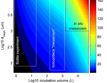
Figure 1.RDR as a function of incubation volume and size of the mesh that was used while filling the incubation volumes (d_mesh).

The black and white boxes illustrate approximate ranges of the three main types of containers used in experiments. Please note that the general definition for mesocosms are volumes≥1000 L (Guangao, 1990) but since most authors also use this term for open batch incubations with volumes between 150–1000 L we also stick to this term for the intermediate class.

cube root ofdmeshwas that in this case the influence ofV /S anddmesh on RDR becomes roughly similar. Figure 1 illus- trates the change of RDR as a function ofV anddmesh. High RDRs are calculated for large-scale in situ mesocosm studies (∼50–190), while bottle experiments yield RDRs between

∼1 and 12.

The key pre-requisite for an experimental parameter to be included in the RDR equation (Eq. 3) was that it is reported in all studies. Many parameters that we would have liked to use for the RDR are either insufficiently reported (e.g. the light environment) or not provided quantitatively at all (e.g. turbu- lence). We therefore had to work with very basic properties related to the experimental setup rather than to the experimental conditions.

A particularly critical aspect of the RDR we had to deal with was the duration of the experiments (Time). Time is re- liably reported in all studies and therefore principally suit- able for the RDR. Our first thoughts were that a realistic community experiment should be long enough to cover relevant ecological processes such as competitive exclusion and therefore also parameterized Time in the first versions of the RDR equation. However, we decided to not account for it in the final version because the factors that define the optimal duration of an experiment are poorly constrained. For example, a 1 d experiment in a 10 L container could indeed miss important CO₂effects caused by food web interactions. On the other hand, a 30 d experiment in the same container could reveal such indirect effects but at the same time be associated with profound bottle effects and make the study unrepresen-

(7)

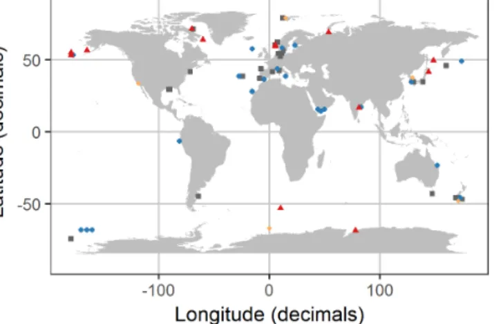
Figure 2.Distribution of experiments with associated OA response of the bulk diatom communities as listed in Table 1. Blue circles indicate positive response; red triangles indicate a negative response;

grey squares indicate no response; orange diamonds indicate a response with unknown direction of change. Locations were slightly modified in case of geospatial overlap to ensure visibility. Please note that the three blue points in the Ross Sea at about−68,−165 are approximate locations because the reference did not provide coordinates.

tative for simulated natural habitat. Thus, too long and too short times are both problematic and the optimum is hard to find. One such attempt to find the optimum Time was made by Duarte et al. (1997), who analysed the plankton ecology literature between 1990 and 1995. By correlating the experimental duration with the incubation volume of published experiments they provided an optimal length for any given volume. However, as noted by Duarte et al. (1997), their cor- relation is based on publication success and therefore rather reflects common practice in plankton ecology experiments and not necessarily a mechanistic understanding of bottle effects. Thus, as there is no solid ground for a parameterization of Time we ultimately decided to not consider it for the RDR.

Finally, we want to point out (and explicitly acknowledge) that the RDR approach to balance the influence of studies on the final outcome of the literature analysis is of course not the one perfect solution and most likely incomplete (see above).

However, balancing a literature analysis with the RDR score may still be an improvement relative to the other case where each experiment is treated exactly equally despite huge differences in the experimental setup. Nevertheless, to account for both views (i.e. the RDR is useless vs. the RDR is useful) we will present the outcome of our literature analysis in two different ways throughout the paper: (1) by simply count- ing the number of outcomes (N) and adding them to yield a cumulativeP

N score (N-based approach; left columns in Figs. 3 and 4) or (2) by adding the RDR score of the experiments with a certain outcome to yield a cumulativeP

RDR score (RDR-based approach; right columns in Figs. 3 and 4).

3 Results

We found 54 relevant publications on CO₂experiments with natural diatom assemblages. Some publications included more than one experiment so that 69 experiments are considered hereafter (Table 1). Most were done with plankton communities from coastal (46 %) and oceanic (28 %) environments. Estuarine and benthic communities were investigated in 16 % and 6 % of the studies, respectively. And 4 % of the studies did not provide coordinates where the samples were taken although the region was reported (Table 1; Fig. 2).

Among the 69 experiments, 23 (33 %,P

RDR=595) revealed a positive influence of CO2on the “bulk diatom community” (see Sect. 2.2), while 13 (19 %,P

RDR=266) revealed a negative one; 5 experiments (7 %, P

RDR=21) found a CO2effect but did not specify whether it is a positive or negative one; and 28 experiments (41 %,PRDR=728) found no effect (Fig. 3a).

We also checked if thepCO₂ range tested in the experiments had an influence on whether the bulk diatom community responded to changing carbonate chemistry. This was done because we expected the likelihood to find an OA response to be higher when the pCO₂ difference between treatments and controls is larger. Thus, we calculated the investigated pCO₂ range (highest pCO₂ – low- estpCO₂) for each experiment and categorized the range into “small” (≤300 µatm), “medium (300–600 µatm), and

“large” (≥600 µatm). Among the 41 experiments that found a CO2effect on the bulk diatom community (positive, negative, and unreported direction of change), 4 (10 %,P

RDR= 106) found it within the low range, 12 (29 %, P

RDR= 123) in the medium range, and 25 experiments (61 %, PRDR=653) in the high range. Among the 28 experiments that found no CO₂on the bulk diatom community, 3 (11 %,PRDR=12) tested within the low range, 8 (29 %, PRDR=230) within the medium range, and 17 experiments (61 %,P

RDR=487) within the high range. Accord- ing to this analysis, the likelihood of detecting a CO₂effect on the bulk diatom community does not depend on the inves- tigatedpCO₂range.

CO₂-dependent shifts in diatom species composition were investigated with light microscopy except for Endo et al. (2015), who used molecular tools. Species shifts were investigated in a subset of 40 of the 69 experiments (Fig. 3b).

Within this subset of 40 studies, 12 (30 %,P

RDR=265) found a shift towards larger diatom species under high CO2, 1 (2.5 %, PRDR=10) found a shift towards smaller diatom species, and 13 (32.5 %,PRDR=67) found no CO₂ effect on diatom community composition. Fourteen studies (35 %,P

RDR=141) reported a CO₂-dependent shift but did not further specify any changes in the size-class distribution (Fig. 3c).

We also tested if the bulk diatom response to OA in coastal, estuarine, and benthic environments was different from the bulk response in oceanic environments. The ra-

2 CO effectsondiatoms:asynthesisofmorethanadecadeofoceanacidiﬁcationexperimentswithnaturalcommunities

CO 2 effects on diatoms: a synthesis of more than a decade of ocean acidification experiments with natural communities

CO ₂ effects on diatoms: a synthesis of more than a decade of ocean acidification experiments with natural communities