Copepod species abundance from the Southern Ocean and other regions (1980–2005) – a legacy

(1)

Earth Syst. Sci. Data, 10, 1457–1471, 2018 https://doi.org/10.5194/essd-10-1457-2018

Copepod species abundance from the Southern Ocean and other regions (1980–2005) – a legacy

Astrid Cornils¹, Rainer Sieger^†, Elke Mizdalski¹, Stefanie Schumacher¹, Hannes Grobe¹, and Sigrid B. Schnack-Schiel^†

1Alfred-Wegener-Institut Helmholtz-Zentrum für Polar- und Meeresforschung, Bremerhaven, Germany

†deceased

Correspondence:Astrid Cornils (astrid.cornils@awi.de) Received: 16 March 2018 – Discussion started: 29 March 2018 Revised: 26 May 2018 – Accepted: 8 July 2018 – Published: 16 August 2018

Abstract. This data collection originates from the efforts of Sigrid Schnack-Schiel (1946–2016), a zooplankton ecologist with great expertise in life cycle strategies of Antarctic calanoid copepods, who also investigated zooplankton communities in tropical and subtropical marine environments. Here, we present 33 data sets with abundances of planktonic copepods from 20 expeditions to the Southern Ocean (Weddell Sea, Scotia Sea, Amundsen Sea, Bellingshausen Sea, Antarctic Peninsula), one expedition to the Magellan region, one latitudinal transect in the eastern Atlantic Ocean, one expedition to the Great Meteor Bank, and one expedition to the northern Red Sea and Gulf of Aqaba as part of her scientific legacy. A total of 349 stations from 1980 to 2005 were archived. During most expeditions depth-stratified samples were taken with a Hydrobios multinet with five or nine nets, thus allowing inter-comparability between the different expeditions. A Nansen or a Bongo net was deployed only during four cruises. Maximum sampling depth varied greatly among stations due to different bottom depths. However, during 11 cruises to the Southern Ocean the maximum sampling depth was restricted to 1000 m, even at locations with greater bottom depths. In the eastern Atlantic Ocean (PS63) sampling depth was restricted to the upper 300 m. All data are now freely available at PANGAEA via the persistent identifier https://doi.org/10.1594/PANGAEA.884619.

Abundance and distribution data for 284 calanoid copepod species and 28 taxa of other copepod orders are provided. For selected species the abundance distribution at all stations was explored, revealing for example that species within a genus may have contrasting distribution patterns (Ctenocalanus,Stephos). In combination with the corresponding metadata (sampling data and time, latitude, longitude, bottom depth, sampling depth interval) the analysis of the data sets may add to a better understanding how the environment (currents, temperature, depths, season) interacts with copepod abundance, distribution and diversity. For each calanoid copepod species, females, males and copepodites were counted separately, providing a unique resource for biodiversity and modelling studies. For selected species the five copepodite stages were also counted separately, thus also allowing the data to be used to study life cycle strategies of abundant or key species.

1 Introduction

Copepoda (Crustacea) are probably the most successful metazoan group known, being more abundant than insects, although far less diverse (Humes, 1994; Schminke, 2007).

They occur in all aquatic ecosystems, from freshwater to marine and hypersaline environments, and from polar waters to hot springs (Huys and Boxshall, 1991). Although copepods

are evolutionary of benthic origin (Bradford-Grieve, 2002), they have also successfully colonised the pelagic marine environment, where they can account for 80 %–90 % of the total zooplankton abundance (Longhurst, 1985). In the South- ern Ocean, copepods are the most important zooplankton organisms next to Antarctic krill and salps, both in abundance and biomass (e.g. Pakhomov et al., 2000; Shreeve et

Published by Copernicus Publications.

(2)

al., 2005; Smetacek and Nicol, 2005; Ward et al., 2014; Tar- ling et al., 2017). In the Southern Ocean, copepods are also the most diverse zooplankton taxon, accounting for more than 300 species (Kouwenberg et al., 2014). However, only a few species dominate the Antarctic epipelagic assemblage:

the large calanoidsCalanoides acutus,Calanus propinquus, Metridia gerlachei, andParaeuchaeta antarctica; the small calanoids Microcalanus pygmaeus andCtenocalanus citer;

and the cyclopoids Oithona spp. and species of the family Oncaeidae (e.g. Hopkins, 1985; Atkinson, 1998; Schnack- Schiel, 2001; Tarling et al., 2017). Together these taxa can comprise up to 95 % of the total abundance and up to 80 % of the total biomass of copepods (Schnack-Schiel et al., 1998).

However, the smaller calanoid species alone can account for up to 80 % of the abundance of calanoid copepods (Schnack- Schiel, 2001). Stage-resolve counts for selected species will also allow future users to study life cycle strategies of abundant or key species.

Numerous studies on zooplankton have been conducted in the past in the Atlantic sector of the Southern Ocean (e.g.

Boysen-Ennen and Piatkowski, 1988; Hopkins and Torres, 1988; Boysen-Ennen et al., 1991; Pakhomov et al., 2000; Du- bischar et al., 2002; Ward et al., 2014; Tarling et al., 2017).

A major zooplankton monitoring programme in the South- ern Ocean is the Continuous Plankton Recorder survey (SO- CPR), providing a large-scale coverage of surface Antarc- tic zooplankton species distribution abundances over the last 25 years (Hosie et al., 2003; McLeod et al., 2010). A recent review summarizes the present knowledge on abundance and distribution of Southern Ocean zooplankton (Atkinson et al., 2012). Especially in the Weddell Sea occurrence data of copepods and other zooplankton species are scarce. One of our aims is to fill this gap with the here-presented data sets from the Southern Ocean, collected by Sigrid Schnack- Schiel (1946–2016) over the period of 1982 to 2005.

In recent years there has been ample evidence that marine ecosystems are greatly affected by climate change and ocean acidification (e.g. Beaugrand et al., 2002; Edwards and Richardson, 2004; Rivero-Calle et al., 2015; Smith et al., 2016). In the Southern Ocean, the pelagic ecosystem is likely to be severely affected by increasing water temperatures and the resulting reduction of sea ice coverage in the Southern Ocean (Zwally, 1994; Smetacek and Nicol, 2005).

It has already been observed over decades that the biomass of Antarctic krill decreases (Atkinson et al., 2004), but lit- tle is known about the environmental effects on copepods.

Within the pelagic ecosystem zooplankton communities and thus copepods are good indicators for ecosystem health and status due to their short life cycles und their rapid response to changing environments (Reid and Edwards, 2001; Chust et al., 2017). Furthermore, they are generally not commer- cially exploited and thus are likely to reflect impacts of environmental changes more objectively. To better understand the effects of environmental change on planktonic copepods, e.g. via biodiversity analyses and ecological niche modelling,

data on species occurrence, abundance and distribution are essential. However, modelling studies are often limited by the scarcity of available plankton data (Chust et al., 2017).

Thus, freely available data sets on abundance and presence or absence of copepod species are of great importance for future studies on environmental changes in the pelagic realm. The data sets presented here on copepod species and life stages (female, male, copepodites) occurrences and abundance from the Southern Ocean, the eastern Atlantic Ocean, the Mag- ellan region and the Red Sea provide a unique resource for biodiversity and modelling studies. They may also help to en- hance our understanding of how the environment (currents, temperature, depths, season) interacts with copepod abundance, distribution and diversity.

2 Methods

2.1 Sampling locations

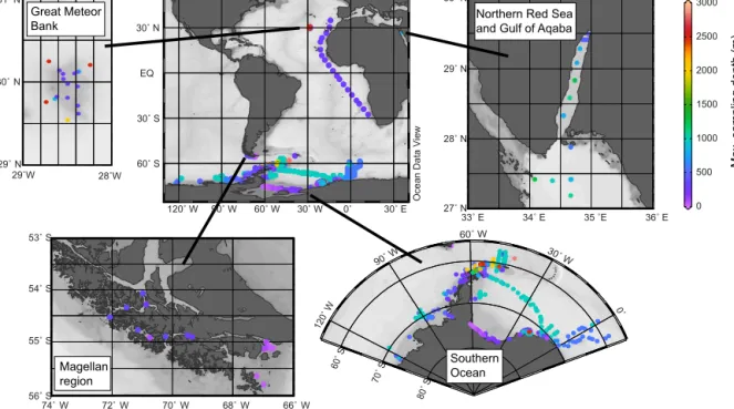
The presented data sets were collected during 24 research cruises with several research vessels from 1980 to 2005 (Ta- ble 1; Cornils and Schnack-Schiel, 2018). Most of the data sets (28 data sets from 20 cruises) are based on samples from the Southern Ocean (Fig. 1), collected on-board R/V Polarstern(25 data sets from 16 cruises), R/VMeteor(1 data set), R/VJohn Biscoe(1 data set) and R/VPolarsirkel(1 data set). Southern Ocean sampling locations were restricted to the Weddell Sea, the Scotia Sea, the Antarctic Peninsula, the Bellingshausen Sea and the Amundsen Sea (Fig. 1).

Additionally, four data sets were collected in other regions (Table 1). In 1994 net samples were collected on-board R/V Victor Hensen in the Magellan region. Two data sets are based on research cruises with R/VMeteor, to the Great Me- teor Bank in the North Atlantic (1998) and to the northern Red Sea and the Gulf of Aqaba (1999). In 2002, plankton net samples were taken during a research cruise with R/V Polarsternalong a transect in the eastern tropical Atlantic Ocean (Table 1).

Maximum sampling depth varied greatly among stations due to different bottom depths (Table 1). However, during 11 cruises to the Southern Ocean the maximum depth was restricted to 1000 m, even at locations with greater bottom depths. In the eastern Atlantic Ocean (PS63) sampling depth was restricted to the upper 300 m.

2.2 Sampling gear

Three types of plankton nets were deployed: Bongo nets, single opening–closing Nansen nets and multiple opening–

closing nets. During all expeditions vertical hauls were taken, thus allowing no movement of the vessel.

(3)

A.Cornilsetal.:CopepodspeciesabundancefromtheSouthernOcean1459 Table 1.Overview of the sampling periods and research cruises. Abbreviations of regions: Antarctic Peninsula (AP), Weddell Sea (WS), eastern Weddell Sea (EWS), Scotia Sea (SCO), Bellingshausen Sea (BS), Amundsen Sea (AS), western Weddell Sea (WWS), eastern Atlantic Ocean (EAO), Magellan region (MR), Great Meteor Bank (GMB), Red Sea (RS); MN:

Multinet. * Data sets with abundance only for non-calanoid copepod species.

Cruise no. Sampling period Region No. of

stations Net type

Max. sampling depth (m)

Mesh size (µm)

DOI of data sets No. of

taxa

Available CTD profiles/information on hydrography

PS04 ANT-II/2

1983-10-24–1983-11-10 AP 14 MN

midi/

Nansen net

1900 200 https://doi.org/10.1594/PANGAEA.876508 110

PS06 ANT-III/3

1985-01-07–1985-02-24 AP, EWS WS AP EWS

30 61 6 4

MN midi Bongo MN midi MN midi

2880 245 400 2500

100/200 300 200 100

https://doi.org/10.1594/PANGAEA.876726 https://doi.org/10.1594/PANGAEA.878275 https://doi.org/10.1594/PANGAEA.878276 https://doi.org/10.1594/PANGAEA.879771

258 28 21 14*

https://doi.org/10.1594/PANGAEA.860066

PS09 ANT-V/1

1986-05-21–1986-05-31 AP 8 MN

midi

1850 200 https://doi.org/10.1594/PANGAEA.876734 162 https://doi.org/10.1594/PANGAEA.860066 PS10

ANT-V/2

1986-07-18–1986-09-05 EWS 18 3

MN midi

600 100 https://doi.org/10.1594/PANGAEA.878277 https://doi.org/10.1594/PANGAEA.878278

22 169

https://doi.org/10.1594/PANGAEA.860066 PS10

ANT-V/3

1986-10-05–1986-11-24 EWS 7

24 MN midi

10*

211

ANT-VII/2

1988-11-09–1988-11-13 SCO 6 MN

midi

1000 200 https://doi.org/10.1594/PANGAEA.879290 172 PS14

ANT-VII/3

1988-11-26–1989-01-04 SCO 11 12

MN midi

192 52

ANT-VII/4

1989-01-17–1989-01-19 SCO 5 MN

midi

ANT-VIII/2

1989-09-14–1989-10-06 WS 12 MN

midi

ANT-IX/2

1990-11-22–1990-12-15 WS 9 MN

midi

ANT-X/3

1992-04-11–1992-05-02 EWS 12 MN

midi

1000 100 https://doi.org/10.1594/PANGAEA.879536 227 PS23

ANT-X/7

1992-12-18–1993-01-16 WS 16 MN

midi

ANT-XI/3

1994-01-28–1994-03-03 BS, AS 20 6

MN midi

220 42*

ANT-XII/4

1995-04-12–1995-04-17 AS 6

5

MN midi

204 35*

ANT-XVIII/5b

2001-04-18–2001-04-30 BS 9 MN

midi

ANT-XX/1

2002-11-02–2002-11-20 EAO 19 MN

midi

300 100 https://doi.org/10.1594/PANGAEA.880927 353 Schnack-Schiel et al. (2010b) PS65

ANT-XXI/2

2003-12-09–2004-01-01 EWS 10 MN

midi

ANT-XXII/2

2004-12-01–2005-01-02 WWS 9 MN

midi

1000 100 https://doi.org/10.1594/PANGAEA.880983 172 https://doi.org/10.1594/PANGAEA.742627

DAE1979/80 1980-01-01–1980-02-08 WS 50 Nansen

net

JB03 1982-02-02–1982-03-02 BS, AP,

SCO

45 Nansen

net

2850 200 https://doi.org/10.1594/PANGAEA.880568 182 https://www.bodc.ac.uk/resources/inventories/cruise_

inventory/report/5916/ (last access: 10 February 2018)

VH1094 1994-11-12–1994-11-24 MR 17 MN

midi

M11/4 1989-12-27–1990-01-08 BS, AP 22 MN

midi

2500 200 https://doi.org/10.1594/PANGAEA.880173 193 https://doi.org/10.1594/PANGAEA.742745

M42/3 1998-09-01–1998-09-16 GMB 17 MN

midi

2500 100 https://doi.org/10.1594/PANGAEA.882283 349 Beckmann and Mohn (2002), Mohn and Beckmann (2002)

M44/2 1999-02-22–1999-03-07 RS 15

5

MN maxi

1300 500

150 https://doi.org/10.1594/PANGAEA.881899 https://doi.org/10.1594/PANGAEA.880901

186 52

Cornils et al. (2005), Plähn et al. (2002)

www.earth-syst-sci-data.net/10/1457/2018/EarthSyst.Sci.Data,10,1457–1471,2018

(4)

80˚ S 60˚ S

90˚ W

60˚ W

30˚ W

0˚

70˚ S 120˚ W

27˚ N 28˚ N 29˚ N 30˚ N

33˚ E 34˚ E 35 ˚E 36˚ E

60˚ S 30˚ S EQ 30˚ N

120˚ W 90˚ W 60˚ W 30˚ W 0˚ 30˚ E Ocean Data View

0 500 1000 1500 2000 2500 3000

56˚ S 55˚ S 54˚ S 53˚ S

74˚ W 72˚ W 70˚ W 68˚ W 66˚ W

31˚ N

30˚ N

29˚ N

29˚W 28˚W

Great Meteor Bank

Magellan region

Southern Ocean

Northern Red Sea and Gulf of Aqaba

Max. sampling depth (m)

Figure 1.Overview of all stations and sampling regions, including the maximum sampling depths (colour scale bar) of the data set.

2.2.1 Nansen net

During the expeditions PS04, DAE1979/80 and JB03 net sampling was carried out with a Nansen net (Table 1). The Nansen net is an opening–closing plankton net for vertical tows (Nansen, 1915; Currie and Foxton, 1956). Thus, it is possible to sample discrete depth intervals to study the vertical distribution of zooplankton. The Nansen net has an opening of 70 cm diameter and is usually 3 m long. Two different mesh sizes were used: 200 µm for the cruises PS04 and JB03, and 250 µm for DAE1979/80. To conduct discrete depth intervals the net is lowered to maximum depth and then hauled to a certain depth and closed via a drop weight. Then the net is hauled to the surface and the sample is removed. This process of sampling depth intervals can be repeated until the surface layer is reached. The volume of filtered water was calculated using the mouth area and depth interval due to the lack of a flowmeter.

2.2.2 Multinet systems

Most presented data sets are based on plankton samples taken with a multinet system (MN) from Hydrobios (Table 1) a revised version (Weikert and John, 1981) of the net described by Bé et al. (1959). The multinet is equipped with five (midi) or nine (maxi) plankton nets, with a mouth area of 0.25 and 0.5 m², respectively. These nets can be opened and closed at depth on demand from the ship via a conductor cable. Thus, they allow sampling of discrete water layers. The net system was hauled at a general speed of 0.5 m s⁻¹. Mesh sizes varied between the data sets from 55 to 300 µm (Table 1). In

the Southern Ocean the mesh sizes were consistent within regions: in the Weddell Sea 100 µm mesh size was used with a few exceptions during PS06. In the Scotia Sea and near the Antarctic Peninsula a mesh size of 200 µm was employed.

In the Bellingshausen Sea and the Amundsen Sea multinet hauls with 55 µm mesh sizes were carried out. In other regions mesh sizes of 100 µm (PS63, M42/3), 150 µm (M44/2) and 300 µm (VH1094) were used. The MN maxi was only deployed during the research cruise M44/2 in the northern Red Sea.

Generally, the volume of filtered water was calculated from the surface area of the net opening (midi: 0.25 m², maxi: 0.5 m²) and the sampling depth interval. For the data sets from PS63, PS65, PS67 and M44/2 a mechanical digital flowmeter was used to record the filtering efficiency and to calculate the abundances (see Skjoldal et al., 2013, p. 4). The flowmeter is situated in the mouth area of the net and mea- sures the water flow, providing more accurate volume values of the filtering efficiency.

2.2.3 Bongo net

During one research cruise (PS06) 61 additional samples were taken with the Bongo net (McGowan and Brown, 1966) to study selected calanoid copepod species. The Bongo net contains two nets that are lowered simultaneously for vertical plankton tows. The opening diameter is 60 cm, and the length of the nets is 2.5 m with a mesh size of 300 µm. The volume of filtering water was recorded with a flowmeter and used for the calculation of abundance.

(5)

A. Cornils et al.: Copepod species abundance from the Southern Ocean 1461 2.2.4 Effects of variable net types and mesh sizes

Quantitative sampling of copepods and zooplankton is chal- lenging. Major sources of error are patchiness, avoidance of nets and escape through the mesh (Wiebe, 1971; Skjoldal et al., 2013). These errors are defined by mesh sizes and net types, in particular the mouth area. The effect of patchiness cannot be investigated here due to the lack of replicates.

To our knowledge the sampling efficiency of the Nansen net and the MN midi have not been compared directly (Wiebe and Benfield, 2003; Skjoldal et al., 2013). However, it has been stated that the catches with Nansen net are considerably lower than with the WP-2 net (Hernroth, 1987), although the WP-2 net is considered as a modified Nansen net with a cylindrical front section of 95 cm and a smaller mouth area (57 cm², Skjoldal et al., 2013). The WP-2 net with 200 µm mesh size however, is in its sampling efficiency, measured as total zooplankton biomass, comparable to the MN midi with 200 µm mesh size (Skjoldal et al., 2013). Thus, it has to be taken into account during future analysis that the abundance values from the Nansen net are not directly comparable to those from the MN midi.

The mesh size has a different effect on the zooplankton catch. It is well known that small-sized copepod species (<1 mm), and thus in particular non-calanoid species (e.g. Oithonidae, Oncaeidae) and also juvenile stages from calanoid copepods (e.g.Microcalanus,Calocalanus,Disco), pass through coarse mesh sizes (≥200 µm), while they are retained in finer mesh sizes (Hopcroft et al., 2001; Paffen- höfer and Mazzocchi, 2003). Thus, abundances of smaller specimens as well as the species and life stage composition may vary considerably, when comparing samples from the Bellingshausen and Amundsen Seas (55 µm mesh size), around the Antarctic Peninsula (200 µm) and the Weddell Sea (100 µm).

2.3 Sample processing and analysis

All samples were preserved immediately after sampling in a 4 % formaldehyde–seawater solution. Samples were stored at room temperature until they were sorted in the labora- tory. The formaldehyde solution was removed, the samples were rinsed and copepods were identified and counted under a stereomicroscope, using a modified mini-Bogorov chamber with high transparency as described in the ICES Zooplankton Methodology Manual (Postel et al., 2000). Abundant species were sorted from one-quarter or less of the sample while the entire sample was screened for rare species. Samples were divided with a Motoda plankton splitter (Motoda, 1959; Van Guelpen et al., 1982). Abundance was calculated using the surface area of the net opening and the sampling depth interval or the recordings of the flowmeter. Samples for re- analysis are only available for the cruises M42/3 and M44/2.

Except for five data sets (Cornils and Schnack-Schiel, 2017; Cornils et al., 2017a, b, c, d) all data sets were sorted

and identified by Elke Mizdalski. Thus, the taxonomic con- cept has been used consistently throughout the data sets.

A wide variety of identification keys and species descriptions have been used to identify the copepods, which cannot all be named here. References for the species descriptions and drawings of all identified marine planktonic species can be found in Razouls et al. (2005–2018). Calanoid copepods were identified to the lowest taxa possible, in general genus or species. Furthermore, for each identified taxon, females, males and copepodite (juvenile) stages were separated. Cy- clopoid copepods were identified to species level in four data sets (Cornils et al., 2017a, b, c, d).

Previously published data sets were revised to ensure consistency of species names throughout the data set collection (Michels et al., 2012; Schnack-Schiel et al., 2007, 2010; Schnack-Schiel, 2010a). In the present compilation we have used the currently acknowledged copepod taxonomy as published in WoRMS (World register of Marine Species, WoRMS Editorial Board, 2018) and in Razouls et al. (2005–2018). Species names have been linked to the WoRMS database, so future changes in taxonomy will be tracked. In the parameter comments the “old”

names are archived that were used initially when the specimens were identified. All used species names can be found in the “Copepod species list” under “Further details” at https://doi.org/10.1594/PANGAEA.884619 or at http://hdl.handle.net/10013/epic.

65463ec2-e309-4d57-8fe3-0cebdd7dce70 (last access:

10 February 2018). We also provided the unique identifier (Aphia ID) from WoRMS (WoRMS Editorial Board, 2018) and notes on the distribution of each species.

When specimens could not be identified due to the lack of identification material, uncertainties in the taxonomy or missing parts, they were summarized under the genus name (e.g. Disco spp., Diaixis spp., Paracalanus spp., Micro- calanusspp.) or family name (e.g. Aetideidae, copepodites).

In most data sets some individuals could not be assigned to any family or genus. These are summarized as Calanoida indeterminata, female; Calanoida indeterminata, male; and Calanoida indeterminata, copepodites.

3 Data sets

3.1 Metadata

Each data set has its own persistent identifier. The metadata are consistent among all data sets, thus ensuring the comparability of the data sets and document their quality.

The following metadata can be found in each data set:

– “Related to” includes the corresponding cruise report, related data sets, and scientific articles of Sigrid Schnack-Schiel and others that have used part of the data previously.

www.earth-syst-sci-data.net/10/1457/2018/ Earth Syst. Sci. Data, 10, 1457–1471, 2018

(6)

– “Other version” in a few cases we have revised a previously published version of the data to ensure consistent species names throughout all data sets (for more information see Sect. 2.3).

– “Projects” shows internal projects or those with exter- nal funding. In the present case all data sets are related to internal projects of the AWI (Alfred Wegener Insti- tut Helmholtz Centre for Polar and Marine Research) research program.

– “Coverage” gives the minimum and maximum values of the georeferences (latitude–longitude) of all stations.

– “Event(s)” comprises a list of station labels, a combination of cruise abbreviation and station number. Lati- tude and longitude of the position (units are in decimals with six decimal places), date and time of start and end of station, and elevation giving the bottom depth. Lati- tude and longitude, date and time and elevation were all recorded by the systems of the respective scientific vessel. The campaign name contains the cruise label (including optional labels), the basis of which is the name of the research vessel. The name of the device contains the net type that was deployed, and the comment may show further details of the station operation.

– “Parameter(s)” is a list of parameters used in the data set with columns containing the full and short name, the unit, the PI (which in this data compilation is always Sigrid Schnack-Schiel, except for one data set (https://doi.org/10.1594/PANGAEA.880239), and the method with a comment. The parameter “Date/Time of event” is not always identical with “Date/Time” given in the event. This is the case when the “Device” in the event is set to “Multiple Investigations” and thus the starting time of all investigations at this event is given. “Date/Time of event”, however, is the time when the plankton net haul started. “Date/Time” recorded on R/V Polarstern and during the cruises M42/3 and JB03 was UTC (Coordinated Universal Time) and during cruise M44/2 local time was recorded (UTC+2). No information on “Date/Time” was found for the cruises DAE1979/80, M11/4 and VH1094. “Elevation” provides information on the bottom depth of the plankton station, if available. Three parameters describe the sampling depths interval. “Depth, water” is the mean depth of the sampled depth interval. “Depth top” and “Depth bot” describe the upper and lower limit of the sampling depth interval, respectively. “Volume” is the amount of water that was filtered during each net tow, calculated either using the mouth area of the net and depth interval or with a flowmeter (Sect. 2.2.2). “Comment” gives the detailed information on the net type, the net number and mesh size.

In the following list of parameters are the copepod taxa for which abundance data were recorded. Calanoid taxa are separated into female, male and copepodites. Species names are consistent throughout all data sets, which ensures the comparability of the data sets. Clicking the link on the species names leads to their respective WoRMS ID (see Sect. 2.3).

The “short names” of each taxon consist of the first letter of the generic name and the name of the species. In nine cases this results in identical short names (Pleuromamma antarctica, Paraeuchaeta antarctica = P. antarctica; Temoropia minor, Temorites minor = T. minor; Chiridius gracilis, Centropages gracilis = C. gracilis; Clausocalanus minor, Calanopia minor = C. minor; Heterostylites longicornis, Haloptilus longicornis = H. longicornis; Scolecithricella abyssalis, Spinocalanus abyssalis = S. abyssalis; Scapho- calanus magnus,Spinocalanus magnus=S. magnus). Thus, we advise to use the full scientific names of these species in further analyses.

3.2 Temporal station distribution

While samples of the Magellan region (November 1994), the Gulf of Aqaba and the northern Red Sea (February–

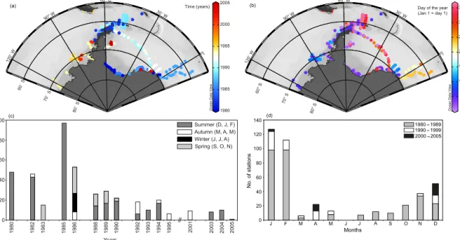
March 1999), the Great Meteor Bank (September 1998), and the eastern Atlantic Ocean (November 2002) were restricted to 1 year and 1 season, the Southern Ocean was sampled multiple times (Table 1). Samples in the Southern Ocean were taken from 1980 to 2005 (Table 1, Fig. 2a, b). The highest number of zooplankton samples was taken in the 1980s (Fig. 2b). In the 1980s the sampling effort was concentrated to the Antarctic Peninsula, the Scotia Sea and the Weddell Sea (Fig. 2a). Samples were taken in multiple years. In the 1990s until 2005 most samples were taken in the Belling- shausen and Amundsen Sea, with fewer samples in the western and eastern Weddell Sea. Two transects were sampled across the Weddell Sea in the 1990s in austral summer and autumn (Fig. 2b). In general, most stations were sampled during summer (December to February), followed by autumn (March to May) and spring (September to November), while winter samples are only available from 1986 in the eastern Weddell Sea (Fig. 2b, c). Summer and autumn samples are widely distributed from the Amundsen Sea to the eastern Weddell Sea (Fig. 2b), while spring and autumn samples are mostly present from the Scotia Sea and eastern Weddell Sea.

Most samples were taken in January and February (Fig. 2d).

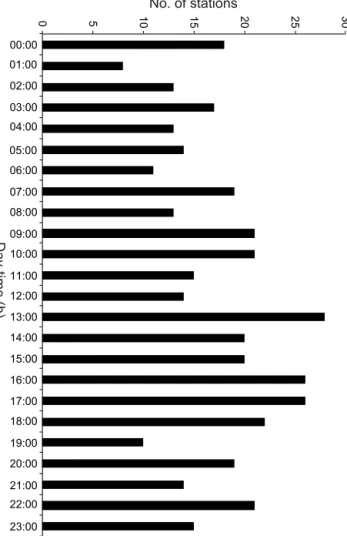
Samples are scattered throughout the entire day (Fig. 3).

It should be taken into account that several copepod species in regions with pronounced seasonality of pri- mary production, e.g. in high latitudes or upwelling regions (Conover, 1988; Schnack-Schiel, 2001), undergo seasonal vertical migration (e.g. Rhincalanus, Calanoides).

They reside in deep water layers during periods of food scarcity and rise to the surface layers when the phytoplank- ton blooms start. Furthermore, other species undergo pronounced diel vertical migrations (e.g.Pleuromamma) from

(7)

A. Cornils et al.: Copepod species abundance from the Southern Ocean 1463

J F M A M J J A S O N D

0 120 100 80 60 40 20

140 1980 1989

1990 1999 2000 2005

No. of stations

Months

Day of the year (Jan 1 = day 1)

1980 1982 1983 1985 1986 1988 1989 1990 1992 1993 1994 1995 2001 2003 2004 2005

0 20 40 60 80 100

Years

No. of stations

Summer (D, J, F) Autumn (M, A, M) Winter (J, J, A) Spring (S, O, N) 70˚S

80˚S

(a) (b)

(c) (d)

70° S 80° S 120˚ W

90° W

60° W

30˚ W

0°

Ocean Data View 0 50 100 150 200 250 300 350

60° S 120˚ W

90° W

60° C

30˚ W

0°

Ocean Data View 1980 1985 1990 1995 2000 2005

60˚S

Time (years)

Figure 2.Sampling effort in the Southern Ocean:(a)station distribution in years,(b)station distribution in the annual cycle,(c)number of stations per year and season,(d)number of stations per month and year.

mesopelagic layers during day-time to avoid predators, mov- ing to epipelagic waters at night to feed (Longhurst and Har- rison, 1989). Thus, to avoid biases in the comparison of the vertical distribution of copepod species, season and day-time should be considered during further analysis of the data sets.

3.3 Copepoda

In total, specimens from six copepod orders were recorded in the compiled data sets.

However, in 29 data sets only calanoid copepods were identified on species level. Specimens of other copepod orders were comprised in families or orders.

3.3.1 Calanoida

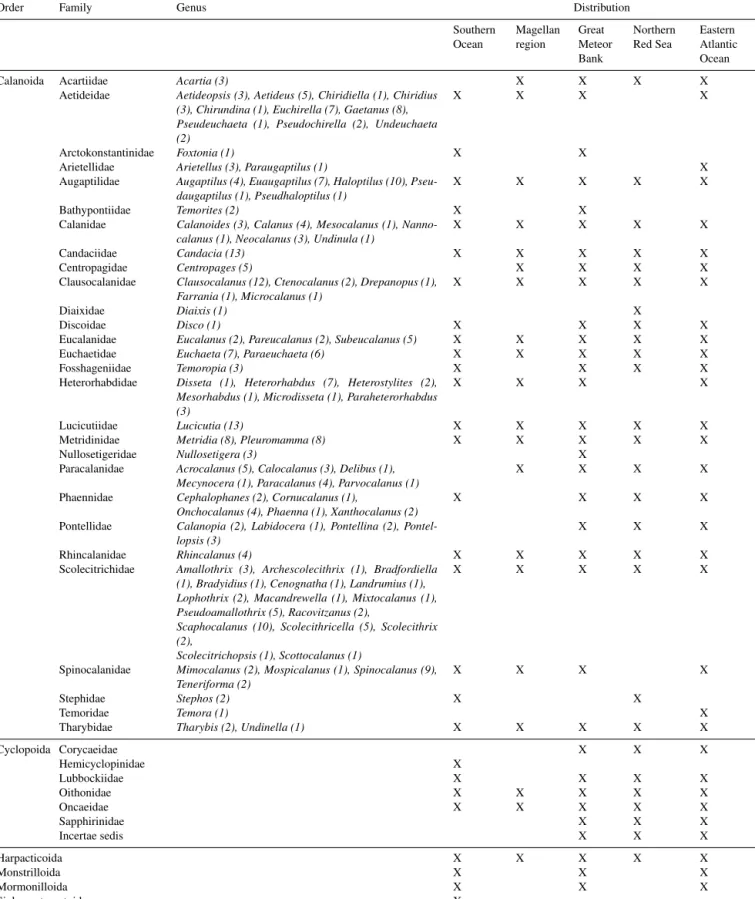
In total 284 calanoid species could be separated into 29 data sets (see “Copepod species list” at https://doi.org/10.1594/PANGAEA.884619). These species are representatives of 28 families and 91 genera (Table 2).

Abundance and distribution data for 96 calanoid species in the Southern Ocean were archived. In the eastern Atlantic Ocean 125 and around the Great Meteor Bank 135 calanoid copepod species could be identified (Table 2). These numbers already indicate the well-known fact that species richness in the tropical and subtropical open oceans is much higher than in the polar Southern Ocean (e.g. Rutherford et al., 1999; Tittensor et al., 2010). Compared to these the number of calanoid species (60) in the subtropical northern Red Sea is low, which is expected due to the shallow sills at the entrance of the Red Sea and the high salinity (see

Cornils et al., 2005). The lowest number of calanoid species (35) was found in the Magellan Region. Calanoid copepod families with the highest number of species were Aetideidae (33), Augaptilidae (27) and Scolecitrichidae (40; Table 2).

For selected species from the Southern Ocean and the northern Red Sea and Gulf of Aqaba, the five copepodite stages were also counted individually (Table 3), providing valuable information on the seasonal and vertical distribution of the five copepodite stages. During four cruises,Rhin- calanus gigasnauplii were also counted (PS09, PS21, PS23, PS29). In the 1990s Sigrid Schnack-Schiel used these data to publish a series of papers on life cycle strategies of Antarctic calanoid copepods such asCalanoides acutus,Rhincalanus gigas,Microcalanuscf.pygmaeusorStephos longipes(e.g.

Schnack-Schiel and Mizdalski, 1994; Schnack-Schiel et al., 1995; Ward et al., 1997; Schnack-Schiel, 2001). However, the stage-resolved copepod data of most species in Table 3 have not been analysed.

It is notable that none of the calanoid species were found in all five regions (see “Copepod species list”

at https://doi.org/10.1594/PANGAEA.884619). In contrast, many species were only recorded in one region: 60 species were found only in the Southern Ocean, while 43 and 38 were found only in the data sets from the Great Meteor Bank and the transect in the eastern Atlantic Ocean, respectively. A total of 24 species were found only in the Red Sea and 6 were identified only from samples in the Magellan region. Of the 28 calanoid families, 11 were distributed in all five regions (Table 2).

As an example of the geographical and vertical distribution of the copepods, three abundant genera were chosen

(8)

Table 2.List of calanoid copepod families and genera, cyclopoid families, and other orders compiled in this data collection. The number of species for each genus is written in parentheses. The presence of the calanoid and cyclopoid families and other copepod orders in the five different regions is marked (X). For a complete overview of all species see the “Copepod species list” at https://doi.org/10.1594/PANGAEA.

884619.

Order Family Genus Distribution

Southern Ocean

Magellan region

Great Meteor Bank

Northern Red Sea

Eastern Atlantic Ocean

Calanoida Acartiidae Acartia (3) X X X X

Aetideidae Aetideopsis (3), Aetideus (5), Chiridiella (1), Chiridius (3), Chirundina (1), Euchirella (7), Gaetanus (8), Pseudeuchaeta (1), Pseudochirella (2), Undeuchaeta (2)

X X X X

Arctokonstantinidae Foxtonia (1) X X

Arietellidae Arietellus (3), Paraugaptilus (1) X

Augaptilidae Augaptilus (4), Euaugaptilus (7), Haloptilus (10), Pseu- daugaptilus (1), Pseudhaloptilus (1)

X X X X X

Bathypontiidae Temorites (2) X X

Calanidae Calanoides (3), Calanus (4), Mesocalanus (1), Nanno- calanus (1), Neocalanus (3), Undinula (1)

X X X X X

Candaciidae Candacia (13) X X X X X

Centropagidae Centropages (5) X X X X

Clausocalanidae Clausocalanus (12), Ctenocalanus (2), Drepanopus (1), Farrania (1), Microcalanus (1)

X X X X X

Diaixidae Diaixis (1) X

Discoidae Disco (1) X X X X

Eucalanidae Eucalanus (2), Pareucalanus (2), Subeucalanus (5) X X X X X

Euchaetidae Euchaeta (7), Paraeuchaeta (6) X X X X X

Fosshageniidae Temoropia (3) X X X X

Heterorhabdidae Disseta (1), Heterorhabdus (7), Heterostylites (2), Mesorhabdus (1), Microdisseta (1), Paraheterorhabdus (3)

X X X X

Lucicutiidae Lucicutia (13) X X X X X

Metridinidae Metridia (8), Pleuromamma (8) X X X X X

Nullosetigeridae Nullosetigera (3) X

Paracalanidae Acrocalanus (5), Calocalanus (3), Delibus (1), Mecynocera (1), Paracalanus (4), Parvocalanus (1)

X X X X

Phaennidae Cephalophanes (2), Cornucalanus (1),

Onchocalanus (4), Phaenna (1), Xanthocalanus (2)

X X X X

Pontellidae Calanopia (2), Labidocera (1), Pontellina (2), Pontel- lopsis (3)

X X X

Rhincalanidae Rhincalanus (4) X X X X X

Scolecitrichidae Amallothrix (3), Archescolecithrix (1), Bradfordiella (1), Bradyidius (1), Cenognatha (1), Landrumius (1), Lophothrix (2), Macandrewella (1), Mixtocalanus (1), Pseudoamallothrix (5), Racovitzanus (2),

Scaphocalanus (10), Scolecithricella (5), Scolecithrix (2),

Scolecitrichopsis (1), Scottocalanus (1)

X X X X X

Spinocalanidae Mimocalanus (2), Mospicalanus (1), Spinocalanus (9), Teneriforma (2)

X X X X

Stephidae Stephos (2) X X

Temoridae Temora (1) X

Tharybidae Tharybis (2), Undinella (1) X X X X X

Cyclopoida Corycaeidae X X X

Hemicyclopinidae X

Lubbockiidae X X X X

Oithonidae X X X X X

Oncaeidae X X X X X

Sapphirinidae X X X

Incertae sedis X X X

Harpacticoida X X X X X

Monstrilloida X X X

Mormonilloida X X X

Siphonostomatoida X

(9)

Table3.ListofspeciesandcruisestotheSouthernOceanwherecopepoditestages1–5wereseparatedandcounted.Specieswithasteriskswereseparatedfromsamplesofcruise M44/2tothenorthernRedSeaandtheGulfofAqaba. SpeciesANT- II/2ANT- III/3ANT- V/1ANT- V/2ANT- V/3ANT- VII/2ANT- VII/3ANT- VII/4ANT- VIII/2ANT- IX/2ANT- X/3ANT- X/7ANT- XI/3ANT- XII/4ANT- XVIII/5bANT- XXI/2ANT- XXII/2M 11/4 Amallothrixdentipes111111 Calanoidesacutus13121121111111111 Calanuspropinquus3121121111111111 Calanussimillimus1211 Ctenocalanusciter111111111111 Heterorhabdusaustrinus111111111111111 Mesocalanustenuicornis* Metridiacurticauda11111211111111 Metridiaspp.(M.gerlachei,M.lucens)131111211111111111 Microcalanusspp.111111111111 Nannocalanusminor* Paraheterorhabdusfarrani111111111111111 Pleuromammaantarctica121 Pleuromammaindica* Pseudoamallothrixcenotelis111111 Rhincalanusgigas12121121111111111 Rhincalanusnasutus* Scolecithricellaminor111111 Spinocalanusantarcticus11111 Spinocalanuslongicornis1111111 Spinocalanusterranovae1111111 Stephoslongipes11111111111 Undinulavulgaris*

(10)

0 5 10 15 20 25 30 00:00

02:00 04:00

06:00 08:00

10:00

12:00 14:00

16:00 18:00

20:00 22:00

Day-time (h)

No. of stations

01:00

03:00

05:00 07:00

09:00 11:00 13:00

15:00

17:00

19:00

21:00

23:00

Figure 3.Sampling effort during day-time in the Southern Ocean.

Day-time is important to understand the behaviour of diel vertical migrators. The number of stations is summarized for every hour of the day, e.g. the bar at 00:00 contains all stations taken between 00:00 and 00:59.

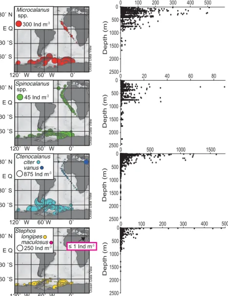
(Fig. 4). WhileMicrocalanusspp. (not separated into species due to uncertainties in the taxonomy) andSpinocalanusspp.

(nine species; Table 2) are abundant down to 1000 m, the two species of Ctenocalanus (two species, Fig. 4) and Stephos occur mainly in the epipelagic layer of the ocean. This is in accordance with their known vertical distribution (Schnack- Schiel and Mizdalski, 1994; Bode et al., 2018). Compar- ing the abundance of SpinocalanusandMicrocalanusfrom all regions suggests that the abundance of these taxa is far greater in the Southern Ocean than in the warmer regions of the ocean. This picture, however, has to be treated with caution, since the tropical Atlantic was only sampled in the upper 300 m of the water column and was thus too shallow for the meso- and bathypelagic genera (Bode et al., 2018).

In the case ofCtenocalanusandStephosour data sets reveal that closely related species within a genus may have contrasting distribution patterns. Stephos longipes and Cteno-

calanus citer are restricted to colder and polar waters of the Southern Hemisphere, whileCtenocalanus vanusoccurs in both the Red Sea and the warm Atlantic Ocean.Stephos maculosusoccurs only in the Red Sea (see arrow in Fig. 4).

Furthermore, the distribution patterns reveal that of the four genera onlyC. citerhas a higher abundance in the samples from the Bellingshausen and Amundsen Seas, and around the Antarctic Peninsula, whileS. longipes,Microcalanusspp.

andSpinocalanusspp. all have higher abundances in the eastern Weddell Sea. This may be due to the lower water depth at the Peninsula since Microcalanus andSpinocalanus are considered as mesopelagic to bathypelagic. Thus, they are often not found at shallow stations (<300 m depth). In case of the sea-ice-associatedS. longipes, low sea-ice conditions and offshore stations may have caused the restricted distribution.S. longipesoccurred mainly in the upper water layers, but it was also recorded with low abundances in deeper layers (Fig. 4). This pattern may be due to its life cycle, shifting seasonally from a sea-ice-associated to a bentho-pelagic life cycle (Schnack-Schiel et al., 1995).

3.3.2 Other Copepoda

In total, 28 non-calanoid taxa were recorded. Four data sets provide only abundance and distribution data for non- calanoid copepod orders (PS06, PS10, PS29, PS35; Ta- ble 1), in particular on species of the order Cyclopoida from the families Oithonidae (two species) and Oncaeidae (six species; Table 2). They were separated into female, male, and copepodite stages 1, 2, 3, 4 and 5. During VH1094 Oithonaspecies were also identified (Table 2). In all other data sets species of these two families were not separated.

In all regions representatives of the family Lubbockiidae were recorded. In the subtropical and tropical samples of PS63, M44/2 and M42/3 abundances of species of the families Corycaeidae and Sapphirinidae, and of the genusPachos were also recorded. Except for PS65, species of the order Harpacticoida were not separated. In the latter five species were identified, mainly sea-ice-associated harpacticoids (Ta- ble 2; Schnack-Schiel et al., 1998). Also, specimens of the orders Monstrilloida, Mormonillida and Siphonostomatoida were counted.

In most data sets, copepod nauplii are also recorded as one parameter. However, due to the small size of nauplii they were not sampled quantitatively and should be discarded in further analysis.

3.4 Further remarks on the usage of the data compilation

Generally, the cruise reports have been linked to each data set. The cruise reports provide valuable information on the itinerary, zooplankton sampling procedures and on other scientific activities on-board that could be useful for the data analysis (e.g. CTD data). Abundance data of selected species

(11)

120˚ W 60˚W 0˚ Ocean Data View

2500 2000 1500 1000 500 0

Depth (m)

2500 2000 1500 1000 500 0

Depth (m)

2500 2000 1500 1000 500 0

Depth (m)

0 100 200 300

0 500 1000 1500

Ocean Data View

60 ˚S 30 ˚S E Q 30˚ N

120˚ W 60˚ W 0˚

60 ˚S 30˚ S E Q 30˚ N 60˚ S 30 ˚S E Q 30˚ N

120˚ W 60˚ W 0˚

60 ˚S 30 ˚S E Q 30˚ N

120˚ W 60˚ W 0˚

Ocean Data View

0 20 40 60 80

Abundance (Ind m^-3)

0 100 200 300 400 500

2500 2000 1500 1000 500 0

Depth (m)

45 Ind m^-3 Spinocalanus spp.

300 Ind m^-3 Microcalanus spp.

250 Ind m^-3 Stephos longipes maculosus

875 Ind m^-3 Ctenocalanus citer vanus

400

≤ 1 Ind m^-3

500

Ocean Data View

Figure 4.Distribution and abundance as individuals per cubic metre (Ind m⁻³) of selected genera (Microcalanus,Spinocalanus,Cteno- calanus,Stephos). Depth (m) is the mean depth of each sampling depth interval (“Depth water”).

and data sets have been published previously in scientific articles. These articles are linked to the respective data sets (under “Related to”).

To use the data, they can be downloaded individually as tab-delimited text files or altogether as a .zip file to allow an import to other software, e.g. R (R core team, 2018) or Ocean Data View (Schlitzer, 2015) for further analysis. Due to the consistent taxonomic nomenclature the individual files can be concatenated easily. It should be kept in mind, however, that not all data sets are directly comparable due to differ- ences in net type and mesh sizes (see Sect. 2.2.4). As noted in Sect. 3.2, several species undergo pronounced seasonal and diel vertical migrations. Therefore, nets from surface waters may not always sample the full vertical extent of the popula- tions, particularly of the biomass dominants.

To evaluate the vertical and spatial distribution of marine plankton, hydrographic information such as temperature and salinity profiles is essential. The relevant publications are available at https://doi.org/10.1594/PANGAEA.884619;

see “Further details”. Recently, a summary of the physical oceanography of R/V Polarstern has been published (Driemel et al., 2017) with CTD data archived in PAN- GAEA as well (Rohardt et al., 2016), except for the cruises PS04 (ANT-II/2), PS14 (ANT-VII/2), PS21 (ANT- X/3), PS63 (ANT-XX/1) and PS65 (ANT-XXII/2) (see Ta- ble 1). For these five cruises information on temperature and salinity profiles exist only for PS63 (Schnack-Schiel et al., 2010) and for PS65 the CTD profiles can be downloaded (https://doi.org/10.1594/PANGAEA.742627; Absy et al., 2008). For M11/4 a CTD data set is also available

(12)

(https://doi.org/10.1594/PANGAEA.742745; Stein, 2010).

To connect the CTD data with the corresponding plankton net haul the metadata “Event“ and “Date/time“ can be used. Furthermore, cruise track and station information are available in the cruise reports as well as on the station tracks for each cruise (https://pangaea.de/expeditions/, last access: 10 February 2018). For the other two R/V Me- teor cruises hydrographic information is available in scientific articles (M42/3: Beckmann and Mohn, 2002; Mohn and Beckmann, 2002; M44/2: Cornils et al., 2005; Plähn et al., 2002). Metadata information of the cruise JB03 can be downloaded from https://www.bodc.ac.uk/resources/

inventories/cruise_inventory/report/5916/ (last access: 10 February 2018). To date, no hydrographic information is publicly available for the cruises DAE79/80 and VH1094.

Additionally, abundances of all other zooplankton organisms in the net samples used for the copepod data sets are available for the four cruises ANT-X/3, ANT-XVIII/5b, M42/3 and M44/2. These can be downloaded at https://doi.org/10.1594/PANGAEA.883833, https://doi.org/10.1594/PANGAEA.884581,

https://doi.org/10.1594/PANGAEA.883771 and https://doi.org/10.1594/PANGAEA.883779.

All data presented here are archived in the database PAN- GAEA. There are, however, other data archiving initia- tives that also store data on copepod abundance and distribution such as COPEPOD (https://www.st.nmfs.noaa.gov/

copepod/, last access: 10 February 2018), BODC (https:

//www.bodc.ac.uk, last access: 10 February 2018) or OBIS (http://www.iobis.org, last access: 10 February 2018). The here-presented data, however, have not been published in any other cataloguing initiative before.

4 Data availability

In total 33 data sets with 349 stations were archived in the PANGAEA^® (Data Publisher for Earth & Envi- ronmental Science, www.pangaea.de) database (Cornils and Schnack-Schiel, 2018). The persistent identifier https://doi.org/10.1594/PANGAEA.884619 links to the splash page of the data compilation. We encourage the users of these data to cite both the DOI of the data collection in PANGAEA as well as the present data publication as a courtesy to Sigrid Schnack-Schiel and the people preparing the data for open access. Metadata include DOIs to cruise reports and related physical oceanography. Data are provided in consistent format as tab-delimited ASCII files and are available through open access under a CC BY license (Creative Commons Attribution 3.0 Unported).

5 Concluding remarks

Pelagic marine ecosystems are threatened by increasing water temperatures due to climate change. These environmental

changes are also expected to cause shifts in the community structure of pelagic organisms. Within the pelagic food web copepods have a central role as intermediator between the microbial loop and higher trophic level. Due to their short life cycles and their high diversity copepods offer a unique opportunity to study effects of environmental variables on numerous taxa with different life cycle strategies. It is also known that their species composition and abundance often reflect environmental changes such as temperature, seasonal variability or stratification (Beaugrand et al., 2002). To understand the complexity of ecological niches and ecosystem functioning, but also to investigate the effects of environmental changes, a detailed knowledge of species diversity, distribution and abundance is essential. The present data compilation provides further information on spatial, vertical and temporal distribution of copepod species and may thus be used to obtain a better picture of species biogeographies. Many individual data sets can also be linked to corresponding CTD profiles (Table 1) and may thus be useful for modelling ap- proaches such as species distribution or environmental niche modelling.

Furthermore, for all calanoid copepods females, males and copepodites were enumerated separately, and for selected species a distinction between copepodite stages was made.

This detailed resolution of abundance data will also allow future investigations on life cycle strategies as well as show how the different stages interact with the environment (e.g.

temperature, currents, depth).

Author contributions. AC and HG were initiators of the data collection and the paper. Data collection and initial analysis was carried out by SiS. Copepod identification (except cyclopoid copepods) and the curation of taxon names was carried out by EM and AC. Data curation was carried out by RS and StS. AC drafted the paper and EM, StS, and HG provided input.

Competing interests. The authors declare that they have no con- flict of interest.

Acknowledgements. We would like to thank numerous sci- entists, technicians and students who helped with the sampling on-board, and the sample processing and analysis in Bremerhaven, in particular Ruth Alheit. We are grateful to the crews of R/Vs Polarstern, Meteor, Victor Hensen, John Biscoeand Polarsirkel, who helped in many ways during every expedition. We would also like to thank Thomas Brey who strongly supported the effort to archive this data collection. Finally, we thank Angus Atkinson and two anonymous reviewers whose comments improved the paper.

Edited by: Falk Huettmann

Reviewed by: Angus Atkinson and two anonymous referees