Highly branched isoprenoids for Southern Ocean sea ice

(1)

https://doi.org/10.5194/bg-16-2961-2019

Highly branched isoprenoids for Southern Ocean sea ice

reconstructions: a pilot study from the Western Antarctic Peninsula

Maria-Elena Vorrath¹, Juliane Müller^1,2,3, Oliver Esper¹, Gesine Mollenhauer^1,2, Christian Haas¹, Enno Schefuß², and Kirsten Fahl¹

1Alfred Wegener Institute, Helmholtz Centre for Polar and Marine Research, Bremerhaven, Germany

2MARUM – Center for Marine Environmental Sciences, University of Bremen, Bremen, Germany

3Department of Geosciences, University of Bremen, Bremen, Germany Correspondence:Maria-Elena Vorrath (maria-elena.vorrath@awi.de) Received: 20 December 2018 – Discussion started: 22 January 2019 Revised: 9 July 2019 – Accepted: 10 July 2019 – Published: 2 August 2019

Abstract. Organic geochemical and micropaleontological analyses of surface sediments collected in the southern Drake Passage and the Bransfield Strait, Western Antarctic Penin- sula, enable a proxy-based reconstruction of recent sea ice conditions in this climate-sensitive area. We study the distribution of the sea ice biomarker IPSO₂₅, and biomarkers of open marine environments such as more unsaturated highly branched isoprenoid alkenes and phytosterols. Comparison of the sedimentary distribution of these biomarker lipids with sea ice data obtained from satellite observations and diatom- based sea ice estimates provide for an evaluation of the suit- ability of these biomarkers to reflect recent sea surface conditions. The distribution of IPSO₂₅ supports earlier suggestions that the source diatom seems to be common in near- coastal environments characterized by annually recurring sea ice cover, while the distribution of the other biomarkers is highly variable. Offsets between sea ice estimates deduced from the abundance of biomarkers and satellite-based sea ice data are attributed to the different time intervals recorded within the sediments and the instrumental records from the study area, which experienced rapid environmental changes during the past 100 years. To distinguish areas characterized by permanently ice-free conditions, seasonal sea ice cover and extended sea ice cover, we apply the concept of the PIP25

index from the Arctic Ocean to our data and introduce the term PIPSO₂₅ as a potential sea ice proxy. While the trends in PIPSO₂₅are generally consistent with satellite sea ice data and winter sea ice concentrations in the study area estimated by diatom transfer functions, more studies on the environmental significance of IPSO₂₅ as a Southern Ocean sea ice

proxy are needed before this biomarker can be applied for semi-quantitative sea ice reconstructions.

1 Introduction

In the last century, the Western Antarctic Peninsula (WAP) has undergone a rapid warming of the atmosphere of 3.7± 1^◦C, which exceeds several times the average global warming (Pachauri et al., 2014; Vaughan et al., 2003). Simultane- ously, a reduction in sea ice coverage (Parkinson and Cav- alieri, 2012), a shortening of the sea ice season (Parkinson, 2002) and a decreasing sea ice extent of∼4 % per decade to 10 % per decade (Liu et al., 2004) are recorded in the adja- cent Bellingshausen Sea. The loss of seasonal sea ice and increased melt water fluxes impact the formation of deep and intermediate waters, the ocean–atmosphere exchange of gases and heat, the primary production, and higher trophic levels (Arrigo et al., 1997; Mendes et al., 2013; Morrison et al., 2015; Orsi et al., 2002; Rintoul, 2007). Since the start of satellite-based sea ice observations, however, a slight increase in total Antarctic sea ice extent has been documented, which contrasts with the significant decrease in sea ice in Western Antarctica, especially around the WAP (Hobbs et al., 2016).

For an improved understanding of the oceanic and atmospheric feedback mechanisms associated with the observed changes in sea ice coverage, reconstructions of past sea ice conditions in climate-sensitive areas such as the WAP are of increasing importance. A common approach for sea ice re-

(2)

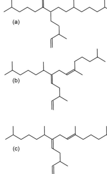
constructions in the Southern Ocean is based on the investigation of sea-ice-associated diatom assemblages preserved in marine sediments (Bárcena et al., 1998; Gersonde and Zielin- ski, 2000; Heroy et al., 2008; Leventer, 1998; Minzoni et al., 2015). By means of transfer functions, this approach can provide quantitative estimates of paleo-sea-ice coverage (Crosta et al., 1998; Esper and Gersonde, 2014a). The application of diatoms for paleoenvironmental studies, however, can be limited by the selective dissolution of biogenic opal frustules (Burckle and Cooke, 1983; Esper and Gersonde, 2014b) in the photic zone (Ragueneau et al., 2000) and in surface sediments (Leventer, 1998). As an alternative or additional approach to diatom studies, Massé et al. (2011) proposed the use of a specific biomarker lipid – a diunsaturated highly branched isoprenoid alkene (HBI C25:2, Fig. 1a) – for South- ern Ocean sea ice reconstructions. The HBI diene was first described by Nichols et al. (1988) from sea ice diatoms.δ¹³C isotopic analyses of the HBI diene suggest a sea ice origin for this molecule (Sinninghe Damsté et al., 2007; Massé et al., 2011) and this is further corroborated by the identification of the sea ice diatomBerkeleya adeliensisas a producer of this HBI diene (Belt et al., 2016). Berkeleya adeliensis is associated with Antarctic landfast ice and the underlying so-called platelet ice (Riaux-Gobin and Poulin, 2004). In a survey of surface sediments collected from proximal sites around Antarctica, Belt et al. (2016) note a widespread sedimentary occurrence of the HBI diene and – by analogy with the Arctic HBI monoene termed IP25 (Belt et al., 2007) – proposed the term IPSO25(ice proxy for the Southern Ocean with 25 carbon atoms) as a new name for this biomarker.

In previous studies, an HBI triene (HBI C25:3; Fig. 1b–c) found in polar and sub-polar phytoplankton samples (Massé et al., 2011) has been considered alongside IPSO₂₅, and the ratio of IPSO₂₅to this HBI triene has hence been interpreted as a measure for the relative contribution of organic matter derived from sea ice algae versus open water phytoplankton (Massé et al., 2011; Collins et al., 2013; Etourneau et al., 2013; Barbara et al., 2013, 2016).

Collins et al. (2013) further suggested that the HBI triene might reflect phytoplankton productivity in marginal ice zones (MIZs) and, based on the observation of elevated HBI triene concentrations in East Antarctic MIZ surface waters, this has been strengthened by Smik et al. (2016a). Known source organisms of HBI trienes (Fig. 1 shows molecular structures of both the E- and Z-isomer) are, for example, Rhizosolenia and Pleurosigma diatom species (Belt et al., 2000, 2017). In the subpolar North Atlantic, the HBI Z-triene has been used to further modify the so-called PIP₂₅ index (Smik et al., 2016b) – an approach for semi-quantitative sea ice estimates. Initially, PIP₂₅ was based on the employment of phytoplankton-derived sterols, such as brassicasterol (24- methylcholesta-5,22E-dien-3β-ol) and dinosterol (4α,23,24- trimethyl-5α-cholest-22E-en-3β-ol) (Kanazawa et al., 1971;

Volkman, 2003), to serve as open-water counterparts, while IP₂₅reflects the occurrence of former sea ice cover (Belt et

Figure 1.The molecular structures of(a)IPSO₂₅,(b)the HBI Z- triene and(c)the HBI E-triene.

al., 2007; Müller et al., 2009, 2011). Consideration of these different types of biomarkers helps to discriminate between ice-free and permanently ice-covered ocean conditions, both resulting in a lack of IP25and IPSO25, respectively (for further details see Belt, 2018 and Belt and Müller, 2013). Uncer- tainties in the source specificity of brassicasterol (Volkman, 1986) and its identification in Arctic sea ice samples, however, require caution when pairing this sterol with a sea ice biomarker lipid for Arctic sea ice reconstructions (Belt et al., 2013). In this context, we note that Belt et al. (2018) reported that brassicasterol is not evident in the IPSO₂₅-producing sea ice diatomBerkeleya adeliensis. While the applicability of HBIs (and sterols) to reconstruct past sea ice conditions has been thoroughly investigated in the Arctic Ocean (Belt, 2018;

Stein et al., 2012; Xiao et al., 2015), only two studies doc- ument the distribution of HBIs in Southern Ocean surface sediments (Belt et al., 2016; Massé et al., 2011). The circum- Antarctic data set published by Belt et al. (2016), however, reports neither HBI triene nor sterol abundances. Signifi- cantly more studies so far focused on the use of IPSO25 and the HBI Z-triene for paleo-sea-ice reconstructions, and these records are commonly compared to micropaleontological diatom analyses (e.g. Barbara et al., 2013; Collins et al., 2013;

Denis et al., 2010).

Here, we provide the first overview of the distribution of IPSO₂₅, HBI trienes, brassicasterol and dinosterol in surface sediments from the permanently ice-free ocean in the area from the Drake Passage to the seasonal sea ice inhabited area of the Bransfield Strait at the northern WAP. Sea ice estimates based on biomarkers are compared to sea ice concentrations

(3)

derived from diatom transfer functions and satellite-derived data on the recent sea ice conditions in the study area. We further introduce and discuss the so-called PIPSO₂₅ index (phytoplankton-IPSO₂₅ index), which, following the PIP₂₅ approach in the Arctic Ocean (Müller et al., 2011), may serve as a further indicator of past Southern Ocean sea ice cover.

2 Oceanographic setting

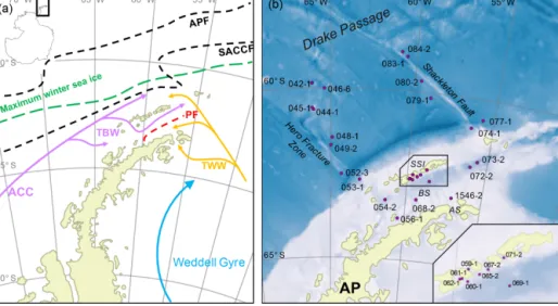
The study area includes the southern Drake Passage and the Bransfield Strait located between the South Shetland Islands and the northern tip of the WAP (Fig. 2a and b).

The oceanographic setting in the Drake Passage is dominated by the Antarctic Circumpolar Current (ACC) and several oceanic fronts showing large geostrophic water mass flows and subduction and upwelling of water masses (Orsi et al., 1995). The Antarctic Polar Front (APF) divides relatively warm subantarctic waters from the cold and salty Antarctic waters, while the southern Antarctic Circumpolar Current Front (SACCF) is often associated with the maximum sea ice extent (Kim and Orsi, 2014). The current system in the Bransfield Strait is relatively complex, and the mixture of water masses is not yet well understood (Mof- fat and Meredith, 2018; Sangrà et al., 2011). A branch of the ACC enters the Bransfield Strait in the west as the Brans- field Current, carrying transitional waters under the influence of the Bellingshausen Sea (Transitional Bellingshausen Sea Water, TBW). The TBW is characterized by a well- stratified, fresh and warm water mass with summer sea surface temperatures (SSTs) above 0^◦C. Below the shallow TBW, a narrow tongue of circumpolar deep water (CDW) flows along the slope of the South Shetland Islands (Sangrà et al., 2011). In the eastern part, transitional water from the Weddell Sea (Transitional Weddell Sea Water, TWW) enters the Bransfield Strait through the Antarctic Sound and from the Antarctic Peninsula (AP). This water mass corresponds to the Antarctic Coastal Current (Collares et al., 2018; Thomp- son et al., 2009). The TWW is significantly colder (summer SST<0^◦C) and saltier due to extended sea ice formation in the Weddell Sea Gyre. The two water masses are separated at the sea surface by the Peninsula Front characterized by a TBW anticyclonic eddy system (Sangrà et al., 2011). While the TWW occupies the deep water column of the Bransfield Strait (Sangrà et al., 2011), it joins the surface TBW in the southwestern Bransfield Strait (Collares et al., 2018).

Due to high concentrations of dissolved iron on the shelf (Klunder et al., 2014), the area around the WAP is characterized by a high primary production with high vertical export fluxes during early summer associated with the formation of fast-sinking mineral aggregates and fecal pellets (Kim et al., 2004; Wefer et al., 1988). The Peninsula Front divides the Bransfield Strait into two biogeographic regimes of high chlorophyll and diatom abundance in the TBW and low chlorophyll values and a predominance of nanoplankton

in the TWW (Gonçalves-Araujo et al., 2015), which is also reflected in the geochemistry of surface sediments (Cárdenas et al., 2018).

3 Materials and methods

3.1 Sediment samples and radiocarbon dating

In total, 26 surface sediment samples obtained by multicor- ers and box corers during the RV Polarstern cruise PS97 (Lamy, 2016) were analysed (Fig. 2, Table 1). All samples were stored frozen and in glass vials. The composition of the sediments ranges from foraminiferal mud in the Drake Pas- sage to diatomaceous mud with varying amounts of ice rafted debris in the Bransfield Strait (Lamy, 2016).

14C radiocarbon dating of two samples from the PS97 cruise and one from thePolarsterncruise ANT-VI/2 (Füt- terer, 1988) was conducted using the mini carbon dating system (MICADAS) at the Alfred Wegener Institute (AWI) in Bremerhaven, Germany, following the method of Wacker et al. (2010). The ¹⁴C ages were calibrated to calendar years before present (cal BP) using the Calib 7.1 software (Stuiver et al., 2019) with an estimated reservoir age of 1178 years, derived from the six closest reference points listed in the Ma- rine Reservoir Correction Database (http://calib.org, last ac- cess: 7 November 2018).

3.2 Organic geochemical analyses

For biomarker analyses, sediments were freeze-dried and ho- mogenized using an agate mortar. After freeze-drying, samples were stored frozen to avoid degradation. The extraction, purification and quantification of HBIs and sterols follow the analytical protocol applied by the international community of researchers performing HBI and sterol-based sea ice reconstructions (Belt et al., 2013, 2014; Stein et al., 2012). Prior to extraction, internal standards 7-hexylnonadecane (7-HND) and 5α-androstan-3β-ol were added to the sediments. For the ultrasonic extraction (15 min), a mixture of CH₂Cl₂:MeOH (v/v 2:1; 6 mL) was added to the sediment. After cen- trifugation (2500 rpm for 1 min), the organic solvent layer was decanted. The ultrasonic extraction step was repeated twice. From the combined total organic extract, apolar hy- drocarbons were separated via open column chromatography (SiO2) using hexane (5 mL). Sterols were eluted with ethylacetate–hexane (v/v 20:80; 8 mL). HBIs were analysed using an Agilent 7890B gas chromatography (30 m DB 1MS column, 0.25 mm diameter, 0.250 µm film thickness, oven temperature 60^◦C for 3 min, increase to 325^◦C within 23 min, holding 325^◦C for 16 min) coupled to an Agilent 5977B mass spectrometer (MSD, 70 eV constant ionization potential, ion source temperature 230^◦C). Sterols were first silylated (200 µL BSTFA; 60^◦C; 2 h; Belt et al., 2013; Brault and Simoneit, 1988; Fahl and Stein, 2012) and then analysed on the same instrument using a different oven tempera-

(4)

Table1.Coordinatesofsamplestationswithwaterdepth,concentrationsofIPSO25,HBIZ-andE-trienes,brassicasterol,anddinosterolnormalizedtoTOC;δ13CvaluesforIPSO25;andvaluesofseaiceindicesPIPSO25basedontheHBIZ-andE-trienes,brassicasterol,anddinosterol.Concentrationsbelowthedetectionlimitareexpressedas0.ThePIPSO25couldnotbecalculatedwhereIPSO25andthephytoplanktonmarkerisabsent(blankfields).

StationLongLatWaterIPSO25/HBIZ-Triene/HBIE-Triene/Brassicasterol/Dinosterol/∂13CofPZIPSO25PEIPSO25PBIPSO25PDIPSO25(◦E)(◦N)DepthTOCTOCTOCTOCTOCIPSO25(m)(µgg−1TOC)(µgg−1TOC)(µgg−1TOC)(µgg−1TOC)(µgg−1TOC)(‰)

PS97/042-1−66.10−59.85417200.3330.15212.99700.0000.0000.000PS97/044-1−66.03−60.62120301.0800143.68800.0000.000PS97/045-1−66.10−60.57229201.5310.38636.90200.0000.0000.000PS97/046-6−65.36−60.00280301.3590.291214.634101.8090.0000.0000.0000.000PS97/048-1−64.89−61.44345502.0850.3751859.60973.5320.0000.0000.0000.000PS97/049-2−64.97−61.67375203.9240.851719.155178.4460.0000.0000.0000.000PS97/052-3−64.30−62.51289000.679026.55400.0000.000PS97/053-1−63.10−62.672021019.3505.94813.356332.8680.0000.0000.0000.000PS97/054-2−61.35−63.2412833.0332.6751.000337.68648.579−14.70.5310.7520.6520.820PS97/056-1−60.45−63.766333.2320.7520.290268.19017.158−10.3±0.90.8110.9180.7160.932PS97/059-1−59.66−62.443540.8352.5231.3053.3860.00020.2490.3900.9810.999PS97/060-1−59.65−62.594621.93412.9374.6935017.4371983.7500.1300.2920.0740.066PS97/061-1−59.80−62.564671.0184.3411.870302.356119.5120.1900.3520.4130.383PS97/062-1−59.86−62.574770.9074.0441.787276.37288.2720.1830.3370.4070.428PS97/065-2−59.36−62.494802.4169.1844.5494788.2921587.3090.2080.3470.0950.100PS97/067-2−59.15−62.427931.7854.0381.710406.567113.7280.3070.5110.4780.533PS97/068-2−59.30−63.1779416.2064.5581.1522096.690653.977−14.1±0.60.7800.9340.6170.643PS97/069-1−58.55−62.59164217.8146.1151.8242472.025774.345−12.6±0.40.7440.9070.6010.626PS97/072-2−56.07−62.01199213.6894.9971.277192.62540.686−13.6±0.30.7330.9150.9370.961PS97/073-2−55.66−61.84262410.3694.2831.4512388.4581180.7520.7080.8770.4760.390PS97/074-1−56.35−60.8718310.37112.0753.4091539.629438.0730.0300.0980.0480.058PS97/077-1−55.71−60.6035872.26716.3564.8741647.616589.7310.1220.3170.2230.219PS97/079-1−59.00−60.15353901.8930.510479.917154.4000.0000.0000.0000.000PS97/080-2−59.64−59.683113012.0212.7054019.0031329.1290.0000.0000.0000.000PS97/083-1−60.57−58.993756018.2568.280686.502308.6100.0000.0000.0000.000PS97/084-2−60.88−58.873617026.85713.8711245.652648.4740.0000.0000.0000.000

(5)

Figure 2. (a)Oceanographic setting of the study area (modified after Hofmann et al., 1996; Sangrà et al., 2011); ACC: Antarctic Circum- polar Current, TBW: Transitional Bellingshausen Water, TWW: Transitional Weddell Water, APF: Antarctic Polar Front, SACCF: Southern Antarctic Circumpolar Current Front and PF: Peninsula Front, and the maximum winter sea ice extent (after Cárdenas et al., 2018).(b)The bathymetric map of the study area with locations of all stations; AP: Antarctic Peninsula, AS: Antarctic Sound, BS: Bransfield Strait and SSI: South Shetland Islands. A detailed station map at the South Shetland Islands is integrated. The overview maps were created with QGIS 3.0 from 2018 and the bathymetry was taken from GEBCO_14 from 2015.

ture programme (60^◦C for 2 min, increase to 150^◦C within 6 min, increase to 325^◦C within 56 min 40 s). As recom- mended by Belt (2018), the identification of IPSO₂₅and HBI trienes is based on comparison of their mass spectra with published mass spectra (Belt, 2018; Belt et al., 2000; see Fig. S1 in the Supplement). Regarding the potential sulfur- ization of IPSO25 we examined the GC-MS chromatogram and mass spectra of each sample for the occurrence of the HBI C25 sulfide (Sinninghe Damsté et al., 2007). The C25

HBI thiane was absent from all samples. For the quantification, manually integrated peak areas of the molecular ions of the HBIs in relation to the fragment ionm/z266 of 7-HND were used. Instrumental response factors are determined by means of an external standard sediment from the Lancaster Sound, Canada. The HBI concentrations in this sediment are known and a set of calibration series was applied to deter- mine the different response factors of the HBI molecular ions (m/z346; m/z348) and the fragment ion of 7-HND (m/z266) (Fig. S2; Belt, 2018; Fahl and Stein, 2012). The identification of sterols was based on comparison of their re- tention times and mass spectra with those of reference compounds run on the same instrument. Comparison of peak areas of individual analytes and the internal standard was used for sterol quantification. The error determined by duplicate GC-MS measurements was below 0.7 %. The detection limit for HBIs and sterols was 0.5 ng g⁻¹sediment. Absolute concentrations of HBIs and sterols were normalized to total organic carbon (TOC) content (for TOC data see Cárdenas et al., 2018).

The herein-presented phytoplankton-IPSO₂₅ index (PIPSO₂₅) is calculated using the same formula as for the

PIP₂₅index following Müller et al. (2011):

PIPSO25= IPSO₂₅

IPSO₂₅+(c×phytoplankton marker). (1) The balance factorc(c=mean IPSO25/mean phytoplankton biomarker) is applied to account for the high offsets in the magnitude of IPSO₂₅and sterol concentrations (see Belt and Müller, 2013, Müller et al., 2011, and Smik et al., 2016b for details and a discussion of thecfactor). Since the concentrations of IPSO₂₅and both HBI trienes are in the same range, thecfactor has been set to 1 (following Smik et al., 2016b).

For the calculation of the sterol-based PIPSO₂₅index using brassicasterol and dinosterol the appliedcfactors are 0.0048 and 0.0137, respectively.

Stable carbon isotope composition of IPSO₂₅, requiring a minimum of 50 ng carbon, was successfully determined on five samples using GC-irm-MS. The ThermoFisher Scientific Trace GC was equipped with a 30 m Restek Rxi-5 ms column (0.25 mm diameter, 0.25 µm film thickness) and coupled to a Finnigan MAT 252 isotope ratio mass spectrometer via a modified GC/C interface. Combustion of compounds was done under continuous flow in ceramic tubes filled with Ni wires at 1000^◦C under an oxygen trickle flow. The same GC programme as for the HBI identification was used. The calibration was done by comparison to a CO₂monitoring gas.

The values ofδ¹³C are expressed in per mille (‰) against Vienna Pee Dee Belemnite (VPDB), and the mean standard deviation was <0.9 ‰. An external standard mixture was measured every six runs, achieving a long-term mean standard deviation of 0.2 ‰ and an average accuracy of<0.1 ‰.

(6)

Stable isotopic composition of neither HBI trienes nor sterols could be determined due to coeluting compounds.

3.3 Diatoms

Details of the standard technique of diatom sample preparation were developed in the micropaleontological laboratory at the AWI in Bremerhaven, Germany. The preparation included a treatment of the sediment samples with hydrogen peroxide and concentrated hydrochloric acid to remove organic and calcareous remains. After washing the samples several times with purified water, the water was removed and the diatoms were embedded on permanent mounts for counting (see detailed description by Gersonde and Zielin- ski, 2000). The respective diatom counting was carried out according to Schrader and Gersonde (1978). On average, 400 to 600 diatom valves were counted in each slide using a Zeiss Axioplan 2 at×1000 magnification. In general preservation state of the diatom assemblages was moderate to good in the Bransfield Strait and decreased towards the Drake Passage where it is moderate to poor.

Diatoms were identified to species or species group level and if possible to forma or variety level. The taxonomy fol- lows primarily Hasle and Syvertsen (1996), Zielinski and Gersonde (1997), and Armand and Zielinski (2001). Follow- ing Zielinski and Gersonde (1997) and Zielinski et al. (1998) we combined some taxa into the following groups.

TheThalassionema nitzschioidesgroup combinesT. nitzschioidesvar.lanceolataandT. nitzschioidesvar.capitulata, two varieties with a gradual transition of features between them and no significantly different ecological response. The species Fragilariopsis curta and Fragilariopsis cylindrus were combined as the F. curta group, taking into account their similar relationship to sea ice and temperature (Armand et al., 2005; Zielinski and Gersonde, 1997). Furthermore, the Thalassiosira gracilisgroup comprisesT. gracilisvar.gracilis and T. gracilis var.expecta because the characteristic patterns in these varieties are often transitional, which ham- pers distinct identification.

Although the two varieties,Eucampia antarcticavar.recta and E. antarctica var.antarctica, display different biogeo- graphical distribution (Fryxell and Prasad, 1990), they were combined to the E. antarctica group. This group was not included in the transfer function (TF) as it shows no relationship to either sea ice or temperature variation (Esper and Gersonde, 2014a, b). Besides the E. antarctica group, we also discarded diatoms assembled as Chaetocerosspp.

group from the TF-based reconstructions, following Zielin- ski et al. (1998) and Esper and Gersonde (2014a). This group combines mainly resting spores of a diatom genus with a ubiquitous distribution pattern that cannot be identified to species level due to the lack of morphological features during light microscopic inspection. Therefore, different ecological demands of individual taxa cannot be distinguished.

For estimating winter sea ice (WSI) concentrations we applied the marine diatom TF MAT-D274/28/4an, comprising 274 reference samples from surface sediments in the western Indian, the Atlantic and the Pacific sectors of the Southern Ocean, with 28 diatom taxa and taxa groups, and an average of 4 analogues (Esper and Gersonde, 2014a). The WSI estimates refer to September sea-ice concentrations averaged over a time period from 1981 to 2010 at each surface sediment site (National Oceanic and Atmospheric Administra- tion, NOAA; Reynolds et al., 2002, 2007). The reference data set is suitable for our approach as it uses a 1^◦ by 1^◦ grid, representing a higher resolution than previously used and results in a root mean squared error of prediction (RMSEP) of 5.52 % (Esper and Gersonde, 2014a). We defined 15 % concentration as threshold for maximum sea-ice expansion following the approach of Zwally et al. (2002) for the presence or absence of sea ice, and 40 % concentration representing the average sea-ice edge (Gersonde et al., 2005; Gloersen et al., 1993). MAT calculations were carried out with the statis- tical computing software R (R Core Team, 2012) using the additional packages Vegan (Oksanen et al., 2012) and Ana- logue (Simpson and Oksanen, 2012). Further enhancement of the sea-ice reconstruction was obtained by consideration of the abundance pattern of the diatom sea-ice indicators, al- lowing for qualitative estimation of sea-ice occurrence, as proposed by Gersonde and Zielinski (2000).

3.4 Sea ice data

The mean monthly satellite sea ice concentration was derived from Nimbus-7 SMMR and DMSP SSM/I-SSMIS passive microwave data and downloaded from the National Snow and Ice Data Center (NSIDC; Cavalieri et al., 1996). The sea ice concentration is expressed to range from 0 % to 100 %, with concentrations below 15 % suggesting the minor occurrence of sea ice. Accordingly, the sea ice extent is defined as the ocean area with a sea ice cover of at least 15 %.

An interval from 1980 to 2015 was used to generate an average sea ice distribution for each season: spring (SON), summer (DJF), autumn (MAM) and winter (JJA) (Table 2), and the data are considered to reflect the modern mean state of sea ice coverage around the WAP. The high standard deviation in the seasonal sea ice concentrations (up to 26 % in winter; Table 2) in the vicinity of the WAP is attributed to the distinct intra- and interannual variability in sea ice coverage.

In this regard, Kim et al. (2005) already related interannual changes in particle flux to annual changes in sea ice cover in the Bransfield Strait. We here suggest that considering mean sea ice concentrations determined for an observational period of 35 years reflects a good estimate of average sea ice conditions and facilitates comparison with sedimentary archives.

(7)

4 Results and discussion

In the following we present and discuss the sedimentary concentrations of IPSO₂₅, HBI trienes and phytosterols regarding their spatial distribution patterns in relation to the environmental conditions and oceanographic features in the study area. We especially focus on the applicability of these biomarkers for reconstructing sea ice conditions and integrate information derived from satellite observations and diatom-based sea ice estimations. We further discuss the possible approach of a sea ice index PIPSO25by analogy with the Arctic sea ice index PIP25(Müller et al., 2011).

4.1 Biomarker distributions in surface sediments 4.1.1 Distribution of IPSO25

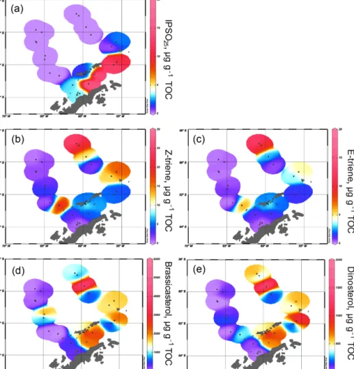
The sea ice biomarker IPSO₂₅ was detected in 14 samples, with concentrations ranging between 0.37 and 17.81 µg g⁻¹ TOC (Table 1). The distribution of IPSO₂₅in the study area shows a clear northwest–southeast gradient (Fig. 3a) with concentrations increasing from the continental slope and around area from the South Shetland Islands to the continental shelf. Maximum IPSO₂₅ concentrations are observed at stations under TWW influence with distinctly cold summer SSTs in the Bransfield Strait. According to Belt et al. (2016), deposition of IPSO25 is highest in areas covered by landfast sea ice and platelet ice during early spring and summer.

Platelet ice is formed under supercooling ocean conditions in the vicinity of ice shelves and subsequently may be incorpo- rated into drifting sea ice (Gough et al., 2012; Hoppmann et al., 2015). We note that, for example, core sites PS97/068, PS97/069, PS97/072 and PS97/073 in the central and eastern Bransfield Strait are located too distal to be covered by fast ice and suggest that peak IPSO₂₅concentrations at these sites may refer to the frequent drift and melt of sea ice exported from the Weddell Sea into the Bransfield Strait. The vertical export of biogenic material from sea ice towards the seafloor may be accelerated significantly by the formation of organic- mineral aggregates, fecal pellets or by (cryogenic) gypsum ballasting, which promotes a rapid burial and sedimentation of organic matter in polar settings (De La Rocha and Passow, 2007; Wefer et al., 1988; Wollenburg et al., 2018). A recent study from Schmidt et al. (2018) shows that the occurrence of IPSO25 in suspended matter and pelagic grazers (krill) is closely linked to the position of the sea ice edge. Lateral subsurface advection of organic matter (including biomarkers) through the TWW, however, may also contribute to elevated IPSO₂₅concentrations at these sites. IPSO₂₅ was not detected in sediments from the permanently ice-free areas in the Drake Passage.

The δ¹³C values of IPSO₂₅ are between −10.3 ‰ and

−14.7 ‰, which is the commonly observed range for IPSO₂₅ in surface sediments, sea-ice-derived organic matter and in Antarctic krill stomachs (Belt et al., 2016; Massé et al., 2011;

Schmidt et al., 2018). These values contrast the low δ¹³C values of marine phytoplankton lipids in Antarctic sediments (−38 ‰ to−41 ‰ after Massé et al., 2011) and support the sea ice origin of IPSO₂₅in the study area.

4.1.2 Distribution of HBI trienes

The HBI Z-triene was present in all 26 samples (0.33–

26.86 µg g⁻¹ TOC) and the HBI E-triene was found in 24 samples (0.15–13.87 µg g⁻¹ TOC) (Table 1). The highest concentrations of both HBI trienes are found in the eastern Drake Passage and along the continental slope, where IPSO25 is absent, while their concentrations in the Brans- field Strait are generally low (Fig. 3b and c), suggesting un- favourable environmental conditions for their source diatoms (e.g. cooler SSTs, sea ice cover, grazing pressure). Contrary to the finding of elevated HBI Z-triene concentrations in surface waters along an ice edge (Smik et al., 2016a) and earlier suggestions that this biomarker may be used as a proxy for MIZ conditions (Belt et al., 2015; Collins et al., 2013;

Schmidt et al., 2018), we observe the highest concentrations of the HBI Z- and E-triene at the permanently ice-free northernmost stations PS97/083 and PS97/084 in the eastern Drake Passage. These core sites are located close to the Antarctic Polar Front (Fig. 2), and we assume that the productivity of HBI triene source diatoms may benefit from mix- ing and upwelling of warm and cold water masses in this area (Moore and Abbott, 2002). Sediments collected south of the Antarctic Polar Front and along the Hero Fracture Zone in the western Drake Passage (Fig. 2) contain moderate and very low concentrations of HBI trienes, respectively. The Hero Fracture Zone is mainly barren of fine-grained sediments and dominated by sands (Lamy, 2016), which may point to inten- sive winnowing by ocean currents impacting the deposition and burial of organic matter. Moderate concentrations of HBI trienes at the continental slope along the WAP (PS97/053, PS97/074, PS97/077) and in the Bransfield Strait likely refer to primary production associated with the retreating sea ice margin during spring and summer. This indicates seasonally ice-free waters in high production coastal areas influenced by upwelling (Gonçalves-Araujo et al., 2015) and feeding of the local food web (Schmidt et al., 2018). The similarity in the distribution of the HBI Z- and the E-triene in our surface sediments – the latter of which is so far not often considered for Southern Ocean paleoenvironmental studies – supports the assumption of a common diatom source for these HBIs (Belt et al., 2000, 2017).

We consider that degradation of biomarker lipids may affect their distribution within surface sediments. While laboratory studies on HBIs in solution point to a low reactiv- ity of IPSO₂₅towards auto- and photooxidative degradation (Rontani et al., 2014, 2011), a more recent investigation into Antarctic surface sediments shows that IPSO₂₅ may potentially be affected by partial autoxidative and bacterial degradation, but oxidation products are found in only minor pro-

(8)

Figure 3.Distribution of(a)IPSO₂₅,(b)HBI Z-triene,(c)HBI E-triene,(d)brassicasterol and(e)dinosterol concentrations normalized to TOC. All distribution plots were made with Ocean Data View (2017).

portions (Rontani et al., 2019a). Since HBI trienes exhibit a generally higher sensitivity to degradation than the C25HBI diene (Rontani et al., 2014, 2019b) – and this is supported by a recent observation of increasing IPSO25/HBI triene ratios with increasing water depths in a polynya system off Eastern Antarctica (Rontani et al., 2019b) – their lower concentrations in the Bransfield Strait have to be considered with care.

Vice versa, regarding maximum HBI triene concentrations and the absence of IPSO₂₅ in Drake Passage sediments, we conclude that the absence of the latter in these samples can be linked to the lack of sea ice (and not to the degradation of IPSO₂₅as HBI trienes would have been removed first).

4.1.3 Distribution of sterols

Brassicasterol is present in all samples, with concentrations ranging from 3.39 to 5017.44 µg g⁻¹TOC, while dinosterol was detected in 22 samples (0.0002–1983.75 µg g⁻¹ TOC).

It is noticeable that the concentrations of sterols exceed the concentrations of IPSO₂₅ and HBI trienes by more than

2 orders of magnitude. We observe higher concentrations of brassicasterol and dinosterol in the eastern part of the Drake Passage, supporting an open marine source for these sterols. Surprisingly, elevated concentrations of brassicasterol are also found at stations PS97/048-1 and 049-2 in the Hero Fracture Zone, which may argue against a winnowing signal, leading to lower accumulation of organic matter. We can only speculate if transport and deposition of re- worked sediment containing brassicasterol via iceberg raft- ing could explain these higher values. In contrast to the observation made for HBI trienes, high sterol concentrations are found in the eastern and central Bransfield Strait (Fig. 3d and e). Previously, elevated concentrations of steroidal com- ponents including brassicasterol and dinosterol in sediment cores from the Bransfield Strait have been interpreted to reflect a high productivity and significant inputs from diatoms and dinoflagellates (Brault and Simoneit, 1988). In a more recent overview, Cárdenas et al. (2018) also report peak concentrations of pigments, sterols and total organic carbon in the Bransfield Strait, which they relate to large seasonal phy-

(9)

toplankton blooms and higher accumulation rates. Dinosterol and, in particular, brassicasterol are known to have different source organisms including diatoms, dinoflagellates, cryptophytes, prymnesiophycean algae and cyanobacteria (Volk- man, 1986), and we assume that this diversity accounts for the higher concentration of these lipids in Bransfield Strait sediments, while concentrations of HBI trienes, mainly derived from diatoms, are significantly lower. Regarding the potential input of brassicasterol from cryptophytes (Gladu et al., 1990; Goad et al., 1983), changes in the dominance of this phytoplankton group over diatoms have been reported for our study area and have been associated with a shallow- ing of the mixed layer and lower salinity due to intensified glacial ice-melting along the WAP (Mendes et al., 2013).

Similar to the observations made for HBIs, selective degradation may also affect the concentration of phytosterols within surface sediments. With respect to the preservation potential of terrigenous and marine derived sterols, Rontani et al. (2012) note only a weak effect of biotic and abiotic degradation of brassicasterol in Arctic Ocean shelf sediments – whether this is also true for Southern Ocean shelf areas needs to be determined. In general, further investigations into degradation processes affecting both HBIs and phytosterols within (the same) sediment samples would address an impor- tant knowledge gap regarding in situ biochemical modifica- tions of the biomarker signal.

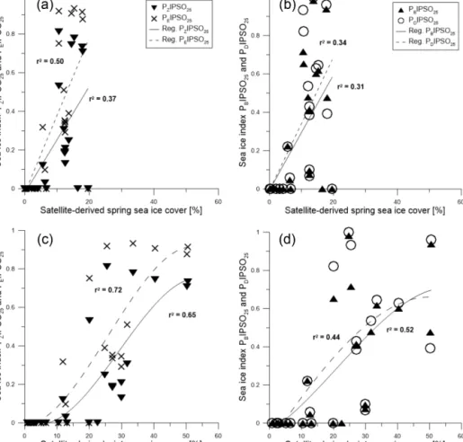
4.2 Comparison of satellite-derived modern sea ice conditions and biomarker data

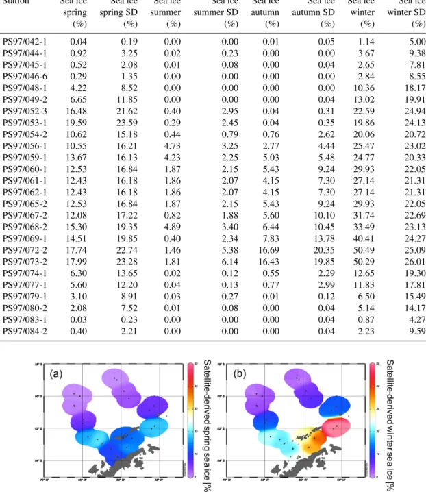
The spring and winter sea ice concentrations are shown in Fig. 4a and b. Winter sea ice is estimated to not extend north of 61^◦S (Fig. 4b) and varies between 1 % and 50 % in the study area, while sea ice is reduced to less than 20 % in spring (Fig. 4a, Table 2). Sea ice concentrations of up to 50 % are common in winter between the South Shetland Is- lands and north of the Antarctic Sound, where the influence of TWW is highest. Permanent sea ice cover is uncommon in the Bransfield Strait and around the WAP and this area is mainly characterized by a high sea ice seasonality, drift ice from the Weddell Sea (Collares et al., 2018) and a seasonally fluctuating sea ice margin.

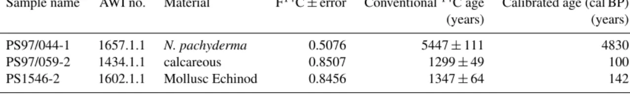
Comparisons of IPSO25and winter sea ice concentrations derived from satellite data reveal a positive correlation (r²= 0.53). The strongest relationship is observed in the eastern Bransfield Strait where the influence of TWW is high. Corre- lations with spring sea ice (r²=0.27) and other seasons are weak. As photosynthesis is not possible and a release of sea ice diatoms from melting sea ice is highly reduced during the Antarctic winter, the observation of a stronger correlation between recent winter sea ice concentrations and IPSO₂₅is un- expected. We hence suggest that this offset may be related to the fact that the sediment samples integrate a longer time interval than is covered by satellite observations. Radiocarbon dating of selected samples that contain calcareous material

reveals an age of 100 years BP in the vicinity of the South Shetland Islands (station PS97/059-2) and 142 years BP at the Antarctic Sound (station PS1546-2, Table 3). A significantly older age was determined for a sample ofN. pachy- dermafrom station PS97/044-1 (4830 years BP) which likely denotes the winnowing and/or very low sedimentation rates in the Drake Passage. Bioturbation effects and uncertainties in reservoir ages potentially mask the ages of the near-coastal samples. Nevertheless, since other published ages of surface sediments within the Bransfield Strait (Barbara et al., 2013; Barnard et al., 2014; Etourneau et al., 2013; Heroy et al., 2008) are also in the range of 0–270 years, we consider that our surface samples likely reflect the paleoenvironmental conditions that prevailed during the last two centuries (and not just the last 35 years covered by satellite observations).

In the context of the rapid warming during the last century (Vaughan et al., 2003) and the decrease in sea ice at the WAP (King, 2014; King and Harangozo, 1998), we suggest that the biomarker data of the surface sediments relate to spring sea ice cover, which must have been enhanced compared to the recent (past 35 years) spring sea ice recorded via remote sensing. Presumably, the average spring sea ice conditions over the past 200 years might have been similar to the modern (past 35 years) winter conditions, which would explain the stronger correlation between IPSO₂₅ and winter sea ice concentrations. The absence of IPSO₂₅at stations PS97/052 and PS97/053, off the continental slope, is in conflict with the satellite data depicting an average winter sea ice cover of 23 %. Earlier documentations that the IPSO25-producing sea ice diatomBerkeleya adeliensisfavours landfast ice communities in East Antarctica and platelet ice occurring mainly in near-coastal areas (Belt et al., 2016; Riaux-Gobin and Poulin, 2004) could explain this mismatch between biomarker and satellite data, which further strengthens the hypothesis that the application of IPSO₂₅seems to be confined to continental shelf or near-coastal and meltwater-affected environments (Belt, 2018; Belt et al., 2016). Alternatively, strong ocean currents (i.e. the ACC) could have impacted the deposition of IPSO₂₅in this region.

Although the distribution pattern of HBI trienes reveals generally higher concentrations in ice-free environments, we note only very weak negative correlations with satellite sea ice data (r²<0.1). This may relate to the strong spatial variability in HBI triene concentrations within the Drake Passage and the different time periods represented by the satellite and sediment data. Similar to the HBI trienes, the sterols also do not show any significant relationship to the satellite sea ice concentrations. High abundances of brassicasterol and dinosterol are observed in both ice-free as well as in seasonally ice-covered regions, which points to a broad environmental adaptation of the source organisms. We hence consider that other environmental parameters than sea ice (e.g. nutrient availability, water temperature and/or grazing pressure) ex- ert major control on the productivity of HBI triene and sterol producers in the study area.

(10)

Table 2.Seasonal sea ice concentrations from satellite observations for spring, summer, autumn and winter, with standard deviations.

Station Sea ice Sea ice Sea ice Sea ice Sea ice Sea ice Sea ice Sea ice spring spring SD summer summer SD autumn autumn SD winter winter SD

(%) (%) (%) (%) (%) (%) (%) (%)

PS97/042-1 0.04 0.19 0.00 0.00 0.01 0.05 1.14 5.00

PS97/044-1 0.92 3.25 0.02 0.23 0.00 0.00 3.67 9.38

PS97/045-1 0.52 2.08 0.01 0.08 0.00 0.04 2.65 7.81

PS97/046-6 0.29 1.35 0.00 0.00 0.00 0.00 2.84 8.55

PS97/048-1 4.22 8.52 0.00 0.00 0.00 0.00 10.36 18.17

PS97/049-2 6.65 11.85 0.00 0.00 0.00 0.04 13.02 19.91

PS97/052-3 16.48 21.62 0.40 2.95 0.04 0.31 22.59 24.94

PS97/053-1 19.59 23.59 0.29 2.45 0.04 0.35 19.86 24.13

PS97/054-2 10.62 15.18 0.44 0.79 0.76 2.62 20.06 20.72

PS97/056-1 10.55 16.21 4.73 3.25 2.77 4.44 25.47 23.02

PS97/059-1 13.67 16.13 4.23 2.25 5.03 5.48 24.77 20.33

PS97/060-1 12.53 16.84 1.87 2.15 5.43 9.24 29.93 22.05

PS97/061-1 12.43 16.18 1.86 2.07 4.15 7.30 27.14 21.31

PS97/062-1 12.43 16.18 1.86 2.07 4.15 7.30 27.14 21.31

PS97/065-2 12.53 16.84 1.87 2.15 5.43 9.24 29.93 22.05

PS97/067-2 12.08 17.22 0.82 1.88 5.60 10.10 31.74 22.69

PS97/068-2 15.30 19.35 4.89 3.40 6.44 10.45 33.49 23.13

PS97/069-1 14.51 19.85 0.40 2.34 7.83 13.78 40.41 24.27

PS97/072-2 17.74 22.74 1.46 5.38 16.69 20.35 50.49 25.09

PS97/073-2 17.99 23.28 1.81 6.14 16.43 19.85 50.29 26.01

PS97/074-1 6.30 13.65 0.02 0.12 0.55 2.29 12.65 19.30

PS97/077-1 5.60 12.20 0.04 0.13 0.77 2.99 11.83 17.81

PS97/079-1 3.10 8.91 0.03 0.27 0.01 0.12 6.50 15.49

PS97/080-2 2.08 7.52 0.01 0.08 0.00 0.04 5.14 14.17

PS97/083-1 0.03 0.23 0.00 0.00 0.00 0.04 0.87 4.27

PS97/084-2 0.40 2.21 0.00 0.00 0.00 0.04 2.23 9.59

Figure 4.The satellite-derived mean sea ice concentrations at each sampling station for(a)spring and(b)winter.

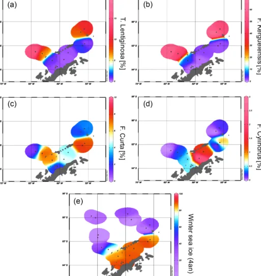
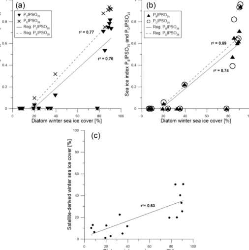
4.3 Comparison of biomarker distributions and diatom-based sea ice estimates

The diatoms preserved in sediments from the study area (Ta- ble 4) can be associated with open-ocean and sea ice conditions (Fig. 5a–d). North of the South Shetland Islands, the strong influence of the ACC is reflected in the high abundance of open-ocean diatom species such as Fragilar- iopsis kerguelensis andThalassiosira lentiginosa (Esper et

al., 2010). The two diatom speciesFragilariopsis curtaand Fragilariopsis cylindrus– known to not produce HBIs (Belt et al., 2016; Sinninghe Damsté et al., 2004) – mark the vicinity to sea ice (Buffen et al., 2007; Pike et al., 2008) and in- dicate fast and melting ice, a stable sea ice margin and strat- ification due to melting processes and the occurrence of seasonal sea ice. These observations are in accordance with previous diatom studies, revealing a dominance ofFragilariop- sis kerguelensisin the permanently open-ocean zone in the

(11)

Table 3.Details of the radiocarbon dates and calibrated ages.

Sample name AWI no. Material F¹⁴C±error Conventional¹⁴C age Calibrated age (cal BP)

(years) (years)

PS97/044-1 1657.1.1 N. pachyderma 0.5076 5447±111 4830

PS97/059-2 1434.1.1 calcareous 0.8507 1299±49 100

PS1546-2 1602.1.1 Mollusc Echinod 0.8456 1347±64 142

Drake Passage and an assemblage shift to more cold-water- adapted and sea-ice-associated species in the seasonal sea ice zone of the Bransfield Strait (Cárdenas et al., 2018).

The high abundance of these sea ice diatoms in our samples is in good agreement with high and moderate IPSO₂₅ concentrations in the Bransfield Strait and around the South Shetland Islands, respectively. The only HBI source diatom identified is the HBI Z-triene-producingRhizosolenia hebe- tata (Belt et al., 2017), which is present in four samples in relatively small amounts and does not show a relation to the measured HBI Z-triene concentrations (Tables 1 and 4). The source diatom of IPSO₂₅ Berkeleya adeliensis was not observed (or preserved) in the samples, and we suggest that additional, hitherto unknown, producers for IPSO25 as well as for the HBI trienes may exist.

We applied the transfer function of Esper and Ger- sonde (2014a) with four analogues (4an, Table 4) to our samples to estimate winter sea ice concentrations (Fig. 5e). The diatom approach shows a clear trend of high winter sea ice concentrations in the range of 78 %–91 % in the Bransfield Strait and low sea ice concentrations (6 %–39 %) north of the continental slope. The fact that diatom data propose sea ice in the Drake Passage may result from the high ages of surface sediments but also from drift, resuspension and sedimentation of diatom remains. Because of the absence of IPSO₂₅in the Drake Passage the correlation of its concentrations with WSI is only weak (r²=0.29).

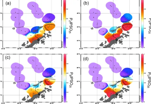
4.4 Testing a semi-quantitative sea ice approach for the Southern Ocean: PIPSO25

Following the PIP25 approach applied in the Arctic Ocean (Müller et al., 2011; Belt and Müller, 2013; Xiao et al., 2015), we used IPSO25, HBI triene and sterol data to calculate the PIPSO25 index. The main concept of combining the sea ice proxy with an indicator of an ice-free ocean environment (i.e.

a phytoplankton biomarker; Müller et al., 2011) aims for a more detailed assessment of the sea ice conditions. By reduc- ing the light penetration through the ice, a thick and perennial sea ice cover limits the productivity of bottom sea ice algae (Hancke et al., 2018), which results in the absence of both sea ice and pelagic phytoplankton biomarker lipids in the underlying sediments. Vice versa, sediments from permanently ice-free ocean areas only lack the sea ice biomarker but contain variable concentrations of phytoplankton biomarkers

(Müller et al., 2011). The co-occurrence of both biomarkers in a sediment sample suggests seasonal sea ice coverage pro- moting algal production indicative of sea ice as well as open- ocean environments (Müller et al., 2011). Consideration of a phytoplankton biomarker alongside the sea ice proxy hence helps to avoid an underestimation of the past sea ice cover deduced from the absence of the sea ice proxy, which, in fact, may also be due to permanent sea ice cover (Belt, 2018, 2019; Belt and Müller, 2013).

Depending on the biomarker reflecting pelagic (open- ocean) conditions, we here define P_ZIPSO₂₅(using the HBI Z-triene), P_EIPSO₂₅(using the HBI E-triene), P_BIPSO₂₅(using brassicasterol) and PDIPSO25(using dinosterol).

The PIPSO25 values are 0 in the Drake Passage and increase to intermediate values at the South Shetland Islands and the continental slope and reach highest values in the Bransfield Strait (Fig. 6a–d). Minimum PIPSO25values are supposed to refer to a predominantly ice-free oceanic environment in the Drake Passage, while moderate PIPSO₂₅ values mark the transition towards a marginal sea ice coverage at the continental slope and around the South Shet- land Islands. Elevated PIPSO₂₅ values in samples from the northeastern Bransfield Strait suggest an increased sea ice cover (probably sustained through the drift of sea ice orig- inating in the Weddell Sea). This pattern reflects the oceanographic conditions of a permanently ice-free ocean north of the South Shetland Islands and a seasonal sea ice zone at the WAP influenced by the Weddell Sea as described by Cárdenas et al. (2018). Both HBI triene-based PIPSO25 in- dices show constantly high values at the coast of the WAP of

>0.7 (PZIPSO25)and>0.8 (PEIPSO25), respectively, and in the southern Bransfield Strait paralleling the southwest–

northeast oriented Peninsula Front described by Sangrà et al. (2011). This front is reported to act as a barrier for phytoplankton communities (Gonçalves-Araujo et al., 2015) and is associated with the encounter between TWW carrying Wed- dell Sea sea ice through the Antarctic Sound and the TBW.

The high PIPSO₂₅values suggesting extended sea ice cover west of the Peninsula Front (station PS97/054 and PS97/056) result from minimum concentrations of pelagic biomarkers and moderate concentrations of IPSO₂₅. PIPSO₂₅values based on the HBI E-triene are about 0.2 higher compared to PZIPSO25, due to the generally lower concentrations of the HBI E-triene (Table 1).

(12)

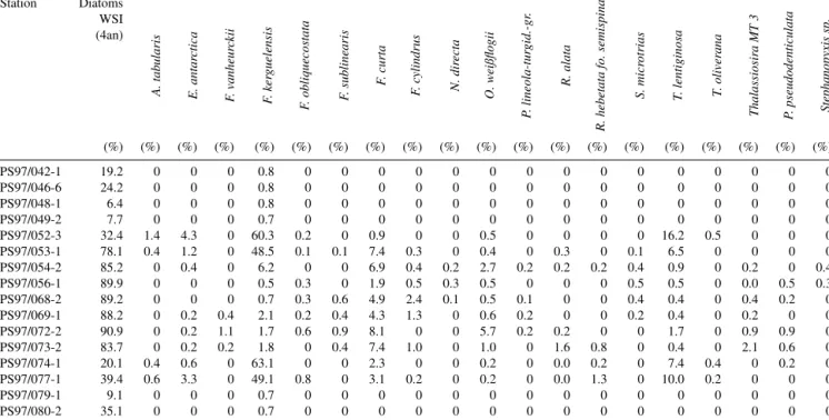
Table 4.Estimations of winter sea ice (WSI) derived from diatom species and the distribution of main diatom species in each sample.

Station Diatoms

A.tabularis E.antarctica F.vanheurckii F.kerguelensis F.obliquecostata F.sublinearis F.curta F.cylindrus N.directa O.weißflogii P.lineola-turgid.-gr. R.alata R.hebetatafo.semispina S.microtrias T.lentiginosa T.oliverana ThalassiosiraMT3 P.pseudodenticulata Stephanopyxissp.

WSI (4an)

(%) (%) (%) (%) (%) (%) (%) (%) (%) (%) (%) (%) (%) (%) (%) (%) (%) (%) (%) (%)

PS97/042-1 19.2 0 0 0 0.8 0 0 0 0 0 0 0 0 0 0 0 0 0 0 0

PS97/046-6 24.2 0 0 0 0.8 0 0 0 0 0 0 0 0 0 0 0 0 0 0 0

PS97/048-1 6.4 0 0 0 0.8 0 0 0 0 0 0 0 0 0 0 0 0 0 0 0

PS97/049-2 7.7 0 0 0 0.7 0 0 0 0 0 0 0 0 0 0 0 0 0 0 0

PS97/052-3 32.4 1.4 4.3 0 60.3 0.2 0 0.9 0 0 0.5 0 0 0 0 16.2 0.5 0 0 0

PS97/053-1 78.1 0.4 1.2 0 48.5 0.1 0.1 7.4 0.3 0 0.4 0 0.3 0 0.1 6.5 0 0 0 0

PS97/054-2 85.2 0 0.4 0 6.2 0 0 6.9 0.4 0.2 2.7 0.2 0.2 0.2 0.4 0.9 0 0.2 0 0.4

PS97/056-1 89.9 0 0 0 0.5 0.3 0 1.9 0.5 0.3 0.5 0 0 0 0.5 0.5 0 0.0 0.5 0.3

PS97/068-2 89.2 0 0 0 0.7 0.3 0.6 4.9 2.4 0.1 0.5 0.1 0 0 0.4 0.4 0 0.4 0.2 0

PS97/069-1 88.2 0 0.2 0.4 2.1 0.2 0.4 4.3 1.3 0 0.6 0.2 0 0 0.2 0.4 0 0.2 0 0

PS97/072-2 90.9 0 0.2 1.1 1.7 0.6 0.9 8.1 0 0 5.7 0.2 0.2 0 0 1.7 0 0.9 0.9 0

PS97/073-2 83.7 0 0.2 0.2 1.8 0 0.4 7.4 1.0 0 1.0 0 1.6 0.8 0 0.4 0 2.1 0.6 0

PS97/074-1 20.1 0.4 0.6 0 63.1 0 0 2.3 0 0 0.2 0 0.0 0.2 0 7.4 0.4 0 0.2 0

PS97/077-1 39.4 0.6 3.3 0 49.1 0.8 0 3.1 0.2 0 0.2 0 0.0 1.3 0 10.0 0.2 0 0 0

PS97/079-1 9.1 0 0 0 0.7 0 0 0 0 0 0 0 0 0 0 0 0 0 0 0

PS97/080-2 35.1 0 0 0 0.7 0 0 0 0 0 0 0 0 0 0 0 0 0 0 0

The sterol-based PIPSO₂₅values display a generally similar pattern to those of PZIPSO25and PEIPSO25, respectively, and we note a high comparability between the PEIPSO25 and PBIPSO25 values (r²=0.73). Some differences, however, are observed in the southwestern part of the Brans- field Strait (station PS97/056), where P_BIPSO₂₅ indicates a lower sea ice cover, and in the central Bransfield Strait (stations PS97/068 and PS97/069), where P_BIPSO₂₅ and P_DIPSO₂₅point to only MIZ conditions. Regarding the modern sea ice conditions, the HBI triene-based PIPSO₂₅ in- dices hence seem to reflect the oceanographic conditions within the Bransfield Strait more satisfactorily. It should be noted that the brassicasterol- or dinosterol-based PIPSO₂₅index links environmental information derived from biomarker lipids belonging to different compound classes (i.e. HBIs and sterols), which have fundamentally different chemical prop- erties. This requires special attention as, for example, selective degradation of one of the compounds may affect the sedimentary concentration of the respective lipids (Rontani et al., 2018). Previous studies linking HBI and sterol-based sea ice reconstructions with satellite-derived or, with respect to downcore paleo-studies, paleoclimatic data, however, demonstrate that the climatic and/or environmental conditions controlling the production of HBIs and sterols seem to exceed the influence of a potential preferential degradation of these biomarkers within the sediments (e.g. Berben et al., 2014; Cabedo-Sanz et al., 2013; Müller et al., 2009, 2012;

Müller and Stein, 2014; Stein et al., 2017; Xiao et al., 2015).

A comparison of PIP₂₅records determined using brassicasterol and the HBI Z-triene for three sediment cores from the

Arctic realm covering the past up to 14 000 years BP (Belt et al., 2015) reveals very similar trends for both versions of the PIP25 index in each core, which may point to, at least, a similar degree of degradation of HBI trienes and sterols through time. More such studies are needed to evaluate the preservation potential of HBIs and sterols in Southern Ocean sediments, especially for down core paleo-studies.

Since brassicasterol and dinosterol are highly abundant in both seasonally ice-covered Bransfield Strait sediments as well as in permanently ice-free Drake Passage sediments, their use as an indicator of fully open-ocean conditions in the study area is questionable. Elevated concentrations of both sterols in the Bransfield Strait could either point to an additional input of these lipids from melting sea ice (Belt et al., 2013) or a better adaptation of some of their source organisms to cooler and/or ice-affected ocean environments.

Production and accumulation of these lipids in (late) summer (i.e. after the sea ice season) has to be considered as well. This observation highlights the need for a better understanding of the source organisms and the mechanisms in- volved in the synthesis of these sterols. Similarly, more research is needed on the production of IPSO₂₅ in Southern Ocean sea ice environments. The source diatomBerkeleya adeliensisseems to be restricted to a very unique ice environment. Previous studies documenting the lack of IPSO₂₅in distal, though winter-sea-ice-covered, areas (e.g. Belt et al., 2016) emphasize this limitation, and it has been suggested that IPSO₂₅ may be more indicative of the type of sea ice rather than sea ice extent (Belt, 2019), which needs to be