Modelling of biospheric CO 2 gross fluxes via oxygen isotopes in a spruce forest canopy: a 222 Rn calibrated box

TELLUS ISSN 0280–6509

Modelling of biospheric CO ₂ gross fluxes via oxygen isotopes in a spruce forest canopy: a ²²² Rn calibrated box

model approach

By UWE LANGEND ¨ORFER¹, MATTHIAS CUNTZ^1,2, PHILIPPE CIAIS², PHILIPPE PEYLIN^2,3, THIERRY BARIAC³, IRENA MILYUKOVA⁴, OLAF KOLLE⁵, TOBIAS NAEGLER¹ and INGEBORG LEVIN¹∗, ¹Institut f¨ur Umweltphysik, Universit¨at Heidelberg (UHEI-IUP), Im Neuenheimer Feld 229, 69120 Heidelberg, Germany;²Laboratoire des Sciences du Climat et de l’Environnement (LSCE), Commisariat `a l’Energie Atomique, L’Orme des Merisiers, Bat 709, 91191 Gif sur Yvette, France;ˆ ³Laboratoire de Biog´eochimie Isotopique (INRA), Universit´e Pierre et Marie Curie, 75005 Paris, France;⁴Servertzov In- stitute of Evolutionary and Ecological Problems (IPEE), Suckachev Laboratory for Biogeocenology, Rus- sian Academy of Sciences, Leninskii pr. 33, 117071 Moscow, Russia;⁵Max-Planck-Institut f¨ur Biogeochemie

(MPI-BGC), Postfach 100 164, 07701 Jena, Germany (Manuscript received 9 July 2001; in final form 18 June 2002)

ABSTRACT

One-dimensional box model estimates of biospheric CO2gross fluxes are presented. The simulations are based on a set of measurements performed during the EUROSIBERIAN CARBONFLUX intensive campaign between 27 July and 1 August 1999 in a naturalPicea abiesforest in Russia. CO2mixing ratios and stable isotope ratios of CO2were measured on flask samples taken in two heights within the canopy. Simultaneously, soil and leaf samples were collected and analysed to derive the¹⁸O/¹⁶O ratio of the respective water reservoirs and the¹³C/¹²C ratio of the leaf tissue. The main objective of this project was to investigate biospheric gas exchange with soil and vegetation, and thereby take advantage of the potential of the¹⁸O/¹⁶O ratio in atmospheric CO2. Via exchange of oxygen isotopes with asso- ciated liquid water reservoirs, leaf CO2assimilation fluxes generally enrich while soil CO2respiration fluxes generally deplete the¹⁸O/¹⁶O ratio of atmospheric CO2. In the model, we parameterised intra- canopy transport by exploiting soil-borne²²²Rn as a tracer for turbulent transport. Our model approach showed that, using oxygen isotopes, the net ecosystem CO2flux can be separated into assimilation and respiration yielding fluxes comparable with those derived by other methods. However, partitioning is highly sensitive to the respective discrimination factors, and therefore also on the parameterisation of internal leaf CO2concentrations and gradients.

1. Introduction

The recent atmospheric budget of carbon dioxide can be balanced only by postulating a significant sink of CO2 in the terrestrial biosphere (Schimel et al., 1996). The characterisation and localisation of this biospheric sink is, however, still a matter of debate

∗Corresponding author.

e-mail: ingeborg.levin@iup.uni-heidelberg.de

(Ciais et al., 1995a,b; Francey et al.,1995; Fan et al., 1998; Bousquet et al., 1999). Recently, the¹⁸O/¹⁶O ratio of atmospheric CO2has evoked scientific atten- tion within the global carbon cycle research because of its unique potential to provide additional infor- mation on carbon exchange between the atmosphere and the terrestrial biosphere, i.e. on the gross carbon fluxes of vegetated areas. Biospheric gas exchange with soil and vegetation modifies the pattern of the

18O/¹⁶O ratio in atmospheric CO2via exchange of oxy- gen isotopes with associated liquid water reservoirs

(Francey and Tans, 1987; Farquhar et al., 1993; Ciais et al., 1997a,b). As leaf CO₂generally enriches and soil CO2respiration fluxes generally deplete the¹⁸O/¹⁶O ratio of atmospheric CO₂, the oxygen isotope compo- sition of CO2carries unique information on the gross fluxes of CO2exchanged by land ecosystems (photo- synthesis, ecosystem respiration), rather than on the net fluxes which are constrained by CO2and¹³C.

There have been several studies on a local scale which investigated the isotopic interaction of CO2and H₂O. Main objective was to study the potential of

18O in CO2and water, to eventually differentiate be- tween assimilation and respiration fluxes (e.g. Yakir and Wang, 1996; Flanagan et al., 1997). Yakir and Wang (1996) estimated separately CO2uptake and res- piration fluxes from small vertical gradients in atmo- spheric CO2and stable isotopes over crop fields. To derive the net fluxes they calculated eddy turbulent ex- change from wind speed profiles and surface character- istics. Flanagan et al. (1997) measured plant stem and leaf water in three major forest types to calculate plant discrimination. They estimated the impact of respira- tion and assimilation fluxes on ecosystem air by cou- pling¹⁸O discrimination with concurrently measured eddy covariance net CO2fluxes, whereby respiration fluxes where estimated from eddy covariance night- time measurements. Here, we present an approach that closes the mass balances for both CO2and theδ¹⁸O- CO2by coupling biospheric exchange fluxes, vertical transport fluxes within the canopy and canopy/CBL (convective boundary layer) exchange fluxes. Our ob- jective is to solve the system of mass balance equa- tions for the assimilation and ecosystem respiration fluxes separately by using measured isotope ratios in canopy air, soil and leaves. The overall net CO2 ex- change (NEE) determined via eddy covariance mea- surements at the top of the canopy (Milyukova et al., 2002) is used as an input of the model which appor- tions the gross fluxes. To parameterise the intra-canopy turbulent transport we use the soil-borne atmospheric

222Rn activity as a tracer.

2. Experimental

2.1. Area of investigation

The measurements were performed during an inten- sive campaign from 27 July to 1 August 1999 in a nat- uralPicea abiesforest in the ‘Central Forest Reserve’

(CFR) at Fyodorovskoe (56^◦27N, 32^◦55E) near Neli-

dovo. The ‘Central Forest Reserve’ is located about 300 km north-west of Moscow in the central part of European Russia, the south-west part of the Valdai upland of the Russian Plain. The forest type at the measurement location is dominated by 36% birch and 20% spruce stocks; 30% consists of a mixture of birch and spruce, 12% is pine and the residual forest consists of alder and deciduous trees (Daniil Kozlov, personal communication). Vegetation is represented by south- ern taiga biota that penetrated into broad-leaved forests of the central part of the Russian Plain. The pattern and characteristics of vegetation cover are primarily controlled by its location in the watershed. The forest understory is dominated by blueberry and sphagnum moss vegetation. The soil profile is rich in humus in the top 50 cm followed by a course loamy soil to a depth of about 1 m. Bogs cover in total 4% of the CFR area. The age of the spruce trees is 181±35 yr with an average height of about 27 m (LAI∼4.3), the understory small shrub and moss layers are dom- inated byVaccinium myrtillus(bilberry, a relative of blueberry) andSphagnum girgensohnii, respectively, hereafter referred to as “blueberries” and “mosses”.

The predominant native wood species (49% of the to- tal CFR area) is spruce (Picea abiesL.) that was not actively used by man before 1931 and after 1960.

2.2. Sampling

Ambient air flask sampling for analysis of CO2mix- ing ratio and stable isotope ratios was installed at the forest tower where the air was sampled from 1.8 and 26.3 m height above ground within and slightly above the canopy (tubing: dekabon furon 1300; pump: KNF Neuberger PM 16029, 24 V). Two preconditioned glass flasks (1.2 L volume each) were flushed with atmospheric air at a flow rate of 2 L min⁻¹for about 30 min and finally pressurised to 1 bar above ambient pressure. Condensation of water vapour in the flask can lead to oxygen isotope exchange of the sampled CO2

with the liquid water (Gemery et al., 1996). There- fore, a cryo-cooling system (a U-shaped glass tube filled with glass bulbs, length about 60 cm, diame- ter about 2 cm, also used for water vapour sampling) prior to a chemical drying column (magnesium per- chlorate) was implemented in the 26.3 m and 1.8 m sampling lines and reduced the vapour pressure of the air streams to a dewpoint of less than –40^◦ C. Dur- ing the whole intensive campaign, a time resolution of 2 h for flask sampling was maintained. These samples were analysed in the Heidelberg laboratory by GC-FID

(gas chromatography – flame ionisation detection) and IRMS (isotope ratio mass spectrometry). In addition, flask sampling during aircraft flights was performed three times per day during early morning, midday and afternoon. The samples were taken at heights of 100, 200, 300, 500, 700, 1000, 1500, 2000, 2500 and 3000 m above ground, and were analysed for CO2mixing ratio and CO2stable isotope ratios at LSCE (Labora- toire des Sciences du Climat et de l’Environnement), Saclay (Ramonet et al., 2002).²²²Rn was measured via its daughter activity with the static filter method at the same heights where flasks were taken with a time resolution of 60 min (Levin et al., 2002). In ad- dition the²²²Rn soil exhalation rate was measured in the footprint of the tower with the inverted chamber method (Levin et al., 2002). On the same soil exhala- tion samples CO2was also measured to determine the soil respiration flux of CO2as well.

To characterise the¹³C and¹⁸O isotopic composi- tion of CO₂exchanged with leaves and soil, in parallel to the flask sampling and continuous²²²Rn measure- ments, bulk leaf and soil material was sampled over the course of the intensive campaign. Sampling fre- quency was 4 h and was synchronised with the tower and aircraft sampling schedule. Deciduous tree leaves and coniferous tree needles have been sampled at two vertical levels (about 10 m and 22 m above ground) as well as moss and blueberry leaves and stems in du- plicate with the same time resolution. Furthermore, once per day (around midday) a trunk wood core of each, the deciduous and the conifer tree was sampled, and a soil core (60 cm depth) underneath each tree.

Net ecosystem CO2exchange was measured with the eddy covariance technique on top of the forest canopy at 28 m height. In addition, vertical CO2 concentra- tion measurements at the tower were performed at 0.2, 1.0, 2.0, 4.8, 10.8, 15.6, 25.2 and 28.0 m, respectively, to determine the CO2concentration profile within the forest canopy at high vertical resolution (Milyukova et al., 2002).

As the¹⁸O signature of water vapour is an impor- tant component of the total¹⁸O balance at the tower site, the water vapour samples from cryogenic drying of the ambient air were used forδ¹⁸O-H2O analysis (time resolution of integrated samples: 4 h). The design of the cold trap (see above) was optimised for mini- mum loss of water vapour at a dewpoint of−40^◦C;

the maximum change of theδ¹⁸O signature was deter- mined not to exceed+0.4‰. For ambient dew points between 10 and 25^◦C, the cooling traps yield a H2O sampling efficiency of more than 99.8%.

2.3. Sample analysis

CO2 mixing ratio on the flasks was measured in Heidelberg with an automated HP 5890 series II gas chromatograph equipped with a methaniser and flame ionisation detector (FID) (Greschner, 1995). The re- producibility of the CO₂concentration analyses (1σ) is better than±0.15 ppm. The stable isotope ratios of the canopy air samples were analysed in the Heidel- berg laboratory with a Finnigan MAT 252 mass spec- trometer, combined with a multiport trapping box for CO2extraction (Neubert, 1998). Typical reproducibil- ity for flask CO2stable isotopes is±0.015‰ (1σ) for δ¹³C and±0.03‰ forδ¹⁸O-CO2. Water vapour sam- ples were stored in the original cold trap and were transferred in the laboratory to the equilibration unit of the mass spectrometer for¹⁸O analysis. The typical reproducibility of theδ¹⁸O-H2O water vapour mea- surement (Finnigan MAT 252) is±0.02‰. Vegetation samples were stored in gas-tight glass bottles. Bulk water was extracted in the vacuum and analysed at the Laboratoire de Biog´eochimie Isotopique, Universit´e Pierre et Marie Curie in Paris (Bariac et al., 1990).

3. Experimental results

3.1. Meteorological parameters

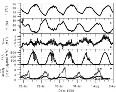
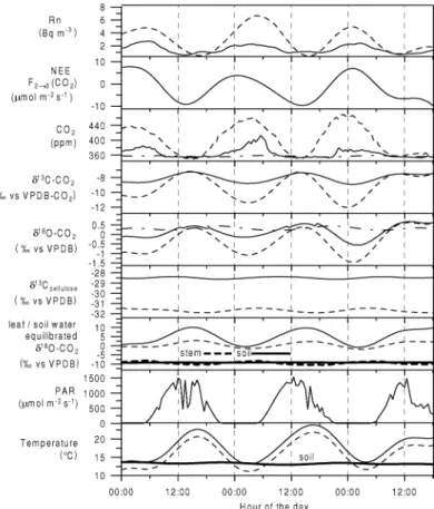
During the 5 day measurement period the overall meteorological conditions are characterised by peri- odic, solar radiation induced diurnal cycles. As shown in Fig. 1, air temperature varied between 12^◦C during night and maximum values of 24^◦C during day, ac- companied by anti-correlated variation of the relative humidity ranging between 85% during night and val- ues of about 30–40% during the day. Also the horizon- tal wind above the canopy at 28 m shows significant diurnal cycles with night-time wind speeds between 1 and 2 m s⁻¹ increasing up to 4 m s⁻¹ during the day. Inspection of photosynthetically active radiation (PAR) clearly exhibits the solar radiation controlled behaviour of the canopy micrometeorology. PAR is zero between 9:40 pm and 4:20 am (local winter time) and reaches maximum values of about 1500 µmol m⁻² s⁻¹ around 1 pm. The observed ²²²Rn activity at 26.3 and 1.8 m height presented in Fig. 1 (lowest panel) also underlies this diurnal, periodic meteorolog- ical pattern. The mean²²²Rn soil exhalation rate for the catchment area of the tower site was determined to be 24±9.7 Bq m⁻²h⁻¹.²²²Rn soil exhalation fluxes

Fig. 1. Meteorological parameters observed during the intensive summer 1999 campaign at a height of 26.3 m: (a) temperature (T), (b) relative humidity (rh), (c) horizontal wind speed (v_h−wind), (d) photosynthetically active radiation (PAR), as well as (e)²²²Rn activity at two heights (26.3 and 1.8 m, error bars indicate 10% statistical counting error).

showed a large variability along a hydrological mea- surement transect, which is due to the dramatically changing groundwater table depth (Levin et al., 2002).

Atmospheric²²²Rn activities at both heights vary with a strong diurnal cycle, caused by an inversion buildup during night. The vertical gradient between top and bottom of the forest canopy then reaches values up to 8 Bq m⁻³. After sunrise, radiative heating initiates convective turbulence which rapidly destroys the ac- cumulated vertical gradient. During day-time,²²²Rn activities at both heights reach similar values, suggest- ing the canopy air to be almost completely well mixed with the CBL.

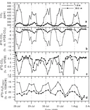
3.2. CO₂mixing ratio and stable isotope ratios Diurnal variations of CO2 mixing ratio and stable isotope ratios at two heights (1.8 and 26.3 m above ground) within the forest canopy measured on the flask samples are shown in Fig. 2. Depending on the mete- orological conditions within the canopy, CO2mixing ratio shows a strong diurnal cycle with maximum con- centrations in the morning and minimum values during the afternoon. During the intensive campaign period, the diurnal CO2amplitude at 1.8 m of 70–120 ppm is much larger than that at 26.3 m, which is only about 20 ppm. The CO2respiration signal at 26.3 m is con- siderably smoothed by the mixing of canopy with CBL

air during day-time, whereas the 1.8 m night time mea- surements strongly reflect the soil respiration flux sig- nal when vertical mixing is suppressed during the build up of night-time inversions.

The diurnal cycles of stable isotopes are anti- correlated to the CO2 concentration cycle, which is expected for bothδ¹³C andδ¹⁸O-CO2. Assuming that the atmospheric CO2 concentration within the forest canopy air,ce, is a two-component mixture of some constant background air concentration,ca, and CO2

that is added or removed by sources and sinks,cs, within the ecosystem, the apparent isotopic signature of the source can be estimated according to:

δe= ca(δa−δs) ce

+δs (1)

whereδaandδsrepresent the isotopic composition of the atmospheric background air and of the source CO2, respectively (Keeling, 1961). This is a linear relation- ship betweenδe and 1/c_e with a slope ofc_a(δa−δs) and an intercept atδsforce→ ∞. Here it is impor- tant to note that this so-called Keeling plot can only be applied on a time scale at which the characteristic iso- topic composition of the sources does not change. On the other hand, the Keeling plot delivers an overall isotopic source signature information, even if the ecosystem source/sink consists of several different components, as long as the relative contribution of

Fig. 2. Diurnal cycles of flask CO2mixing ratio (a),δ¹³C-CO2(b),δ¹⁸O-CO2(c) andδ¹⁸O-H2O of atmospheric water vapour (d) during the summer campaign in 1999 at two sampling heights, 26.3 and 1.8 m above ground.

each component does not change with time. The Keel- ing approach was used first to identify the contribu- tions to the seasonal cycle (Keeling, 1961; Mook et al., 1983). More recently the identification of the iso- topic composition of sources/sinks was also applied to terrestrial ecosystems (Buchmann et al., 1998; Yakir and Sternberg, 2000). The meanδ¹³C source signa- tures derived from the correlation with the inverse CO2

concentration for both heights [during day-time (con- centration decrease) and night-time (concentration in- crease)] are given in Table 1.

The two-component mixing approach yields a con- sistent picture for the diurnal change of the δ¹³C apparent source signature within the canopy. For both heights the same source signatures of about

−24.8‰ vs. VPDB-CO2within a 1σuncertainty range were observed during day-time. During night-time the source is more depleted by about 1.8‰ to−26.6‰

(Table 1). Thisδ¹³C day-time source signature illus-

Table 1. δ¹³C Source signatures and their standard deviations derived from canopy observations^a

δ¹³s C (‰vs. VPDB-CO2)

Period^b 1.8 m height 26.3 m height

Overall −25.94±0.1 −25.68±0.4

Day-time mean −24.79±0.5 −24.73±0.4 Night-time mean −26.39±0.4 −26.82±1.5

aAccepted correlation coefficient r² used for the mean values:r²>0.95.

bDay-time: 7:00–19:00 local winter time. Night-time:

21:00–5:00 local winter time.

trates the strong assimilation discrimination influence on the ecosystem ambient CO2. Assimilation enrich- ment can also be observed forδ¹⁸O-CO2, whereby the anticorrelation to the CO2concentration variabil- ity is not as close as it is forδ¹³C. Due to the isotopic

equilibration exchange of oxygen isotopes with dif- ferent water pools within the ecosystem, there is not necessarily a two-component mixing, and therefore no linear correlation between CO₂ andδ¹⁸O-CO₂ is expected.

3.3. ¹⁸O/¹⁶O in the water pools

The variation of the 4 h integral water vapour δ¹⁸O-H2O within the canopy is presented in Fig. 2d.

A huge diurnal cycle and a vertical gradient are ob- served. Compared to the 1.8 m level, at 26.3 mδ¹⁸O of water vapour is always more depleted with a diur- nal cycle between−19.5 and−22‰ (vs. VSMOW).

The 1.8 m level shows a larger diurnal cycle than the 26.3 m level with most depleted values of about−20‰

during day and enriched values up to−16‰ during night. This diurnal cycle, as well as the vertical pro- file, can be interpreted as the mixture of evaporating soil and leaf water and tropospheric water vapour be- ing significantly depleted compared to the evaporating water. As the evaporating soil water (δ¹⁸O-H₂O about

−11‰ vs. VSMOW, Fig. 3a) should result in a water vapourδ¹⁸O-H2O of about−21‰, due to evaporation fractionation, a large portion of the evaporating water must originate from enriched reservoirs, i.e. from the leaves or condensed surface water on the plant leaves.

0 0 :00 0 6 :0 0 1 2 :0 0 1 8 :00

J u ly 2 9 /3 0 1 9 9 9 -3 3

-3 2 -3 1 -3 0 -2 9 -2 8 -2 7

13C cellulose (‰ vs VPDB) -1 2

-8 -4 0 4 8 1 2

δ18O-H2O (‰ vs VSMOW )

co n ife r lo w co n ife r m e d iu m co n ife r h ig h d e cid u o u s lo w d e cid u o u s h ig h b lu e b e rry le a ve s b lu e b e rry ste m m o ss le a v e s m o ss ste m w o o d co n ife r w o o d d e cid iu s so il co n ife r 5 cm d e p t h so il d e cid u o u s 5 cm d e p t h

a

b

δ

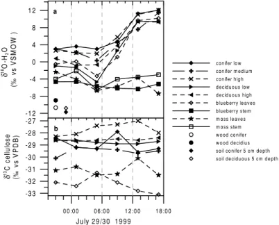
Fig. 3. Diurnalδ¹⁸O-H2O variations of the different vegetation water pools along with soil and trunkδ¹⁸O-H2O (a) and diurnalδ¹³C variations of plant tissue material (b).

Two major schemes of the spatial and temporal evo- lution of theδ¹⁸O-H₂O composition of the vegetation and soil water pools are shown in Fig. 3a. Throughout the day, there is a general enrichment of the¹⁸O/¹⁶O ratio from the bottom to the top of the ecosystem wa- ter pools. The soil water in the top layer of the soil (0–5 cm depth) has aδ¹⁸O-H2O value of−11.25‰

(vs. VSMOW) (mean between soil under coniferous and deciduous dominated areas), whereby the soil wa- ter becomes depleted to about−12.2‰ at a depth of 40 cm, to stay nearly constant down to 60 cm depths (not shown in Fig. 3a). The mean (conifer and decid- uous tree) stem water¹⁸O/¹⁶O ratio of−9.8‰ is en- riched compared to the soil water by about 2‰. Stem water is assumed to represent theδ¹⁸O-H2O of sap wa- ter that is delivered to leaves where it evaporates. For night-time with no assimilation activity, the enrich- ment can further be observed via the understory veg- etation (mosses stem and leaves and blueberry stem) with an¹⁸O/¹⁶O ratio from about−5‰ to−2‰, fol- lowed by the blueberry leaves and the deciduous low level leaves with an¹⁸O/¹⁶O ratio around 0‰. Highest values forδ¹⁸O-H2O during night-time between 0‰

and+4‰ can be observed for the high and low levels of the coniferous needles as well as for the deciduous high level leaves. This reflects the fact that leaf water in trees does not relax back to the stem water isotope

composition during the night in the absence of assim- ilation. The second dominant pattern of the¹⁸O signa- ture in the water pools is the difference in their diurnal cycles. Basically, the vertical gradient is maintained, but except for the blueberry and moss stems and the moss leaves, a strong enrichment of about 10‰ during day-time is detected for all other leaf compartments within the tree leaves.

The¹³C/¹²C ratios of the plant cellulose are pre- sented in Fig. 3b. As expected, no pronounced diurnal cycle can be observed for¹³C of the plant tissue. How- ever, there is a clear vertical gradient towards more enriched values beginning from the understory blue- berries and mosses (δ¹³C = −31 to−33‰) to the respective levels of the tree leaves (δ¹³C= −27 to

−30‰). This principal vertical gradient can be due to a higher assimilative re-fixation rate of soil respired and therefore more depleted CO2for understory vegetation compared to the upper canopy tree leaves, which as- similate more enriched CO₂originating from the CBL.

4. δ¹⁸O Model set-up

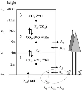
The main objective of the modelling approach is to investigate the potential of the¹⁸O isotopic compo- sition of carbon dioxide and associated water pools to determine the gross CO2 fluxes of the ecosys- tem. As the δ¹⁸O-CO₂ variability within the forest canopy is controlled by both, transport-driven ex- change of canopy CO2 with the CBL and process- related biospheric activity impact, the model has to be well parameterised with respect to transport before the biological processes can be investigated. A one- dimensional box-model set-up was chosen to differ- entiate between the respective carbon dioxide and wa- ter pools, whereby three boxes with quasi-logarithmic height scaling from bottom to top are investigated for their turbulent transport and assimilative and respira- tive exchange fluxes (Fig. 4). The lowest box (box 1, from soil surface to 4 m height) represents the interface with the soil and the understory vegetation regime, the second box (box 2, from 4 m to 26 m height) represents the deciduous and coniferous tree activity within the canopy, whereas box 3 (box 3, from 26 m to 400 m) represents the CBL. Box 2 communicates with box 3 and box 1 via turbulent exchange.

4.1. CO2mass balance

Setting up a mass balance to describe formally the respective CO2fluxes, it is useful to consider a column

4m 15m

2m 400m

1 2 3

R_soil z₁

z₂

R_a1 R_a2

A₁ A₂ K₁₂

F₂₃(CO₂) CO₂, δ¹⁸Ο

CO₂, δ¹⁸Ο, ²²²Rn

CO₂, δ¹⁸Ο, ²²²Rn

F_soil(Rn) z₀

26m z₃

height

R₁= R_soil + R_a1 213m

Fig. 4. Scheme of the canopy box model set-up: the mea- sured input values are in bold characters, the calculated model output values are in normal characters.

of air extending from the soil surface to a height,H, within or above the canopy. The mass balance of CO2

in such an air column within an ecosystem canopy, in case of no horizontal advection of CO₂, is given by eq. (2) [the convention for the algebraic signs are:

inward fluxes (into the canopy column) are calculated positive, outward fluxes negative]:

H Vmol

·d[CO2]

dt = −A+R+Fae(CO2) (2) whereVmolis the molar volume of air [m³mol(air)⁻¹], His the height of the air column (m), [CO₂] is the aver- age mole fraction of CO2within the column [mol(CO2) mol(air)⁻¹],Ris the CO2 respiration flux, given by Rsoil+Ra[mol (CO2) m⁻²h⁻¹],Rsoilis the CO2res- piration flux from soil (heterotrophic and autotrophic) [mol (CO2) m⁻²h⁻¹],Rais the above-ground CO2res- piration flux [mol (CO2) m⁻² h⁻¹],Ais the net CO2

assimilation flux by the foliage within the column [mol (CO2) m⁻² h⁻¹], andFaeis the flux of CO2between the air column and the atmosphere above (mol [CO2) m⁻²h⁻¹].

Within a canopy, it is a priori not the case, and in fact never observed in reality, that there is no gra- dient of CO2 concentration within a column of air from a heightzto a heightz+z. Depending on the canopy structure and meteorological conditions, there

is usually a typical strong night-time gradient of up to 100µmol(CO₂) /mol(air) between bottom and top due to suppressed vertical mixing. Therefore, the average mixing ratio

[CO2(z)]= 1 zmax−zmin

zmax z_min

[CO2(z)] dz (3) must be calculated, to avoid a possible CO2 storage term being missing in eq. (2). To parameterise the intra- canopy turbulent transport between box 1 and box 2 we used the soil-borne atmospheric²²²Rn activity as a tracer. The²²²Rn flux from the lowermost canopy box, box 1, to the adjacent canopy box 2 can be calculated using the mean measured soil²²²Rn exhalation rate Fsoil(Rn), and the atmospheric²²²Rn activity change with time in box 1:

H1

dRn1

dt = Fsoil(Rn)−F12(Rn). (4) In analogy to Fick’s first law, the turbulent diffusion coefficient,K12, can be formulated via the measured vertical²²²Rn gradient between box 1 and box 2 and the distance between the box centreszaccording to:

K12= F12(Rn)z

(Rn1−Rn2) (5)

Mean²²²Rn activities and CO2mixing ratios for each canopy box are calculated by integration of the mea- sured CO2profiles (Milyukova et al., 2002), assuming a similarity between²²²Rn and CO2, with:

[CO_2profile]= 1 zmax−zmin

zmax zmin

[CO_2profile(z)] dz. (6) The CO2 flask mixing ratios and ²²²Rn activities, which are both measured at heightsz=1.8 andz= 26.3 m, respectively, are subsequently scaled to their mean value of each box by assuming:

[CO2flasks]= [CO2profile]

[CO2profile(z)][CO2flasks(z)] (7) and

Rn= [CO2profile]

[CO_2profile(z)]Rn(z). (8)

The isotopes measured at both heights are assumed to represent the mean box values. The CO2flux between box 1 and box 2 is then calculated using the²²²Rn- derivedK12via [see eqs. (4) and (5)]:

F12(CO2)=K12

[CO₂]₁−[CO₂]₂

zV_mol . (9)

As shown in Fig. 1e, within the measurement uncer- tainty of about 10% there is always a negative gradient in²²²Rn activity between bottom and top of the canopy.

Therefore, the exchange coefficientK₁₂will always be positive as long as there is a positive fluxF12(Rn) from box 1 to box 2 in eq. (4). The CO2 flux from box 2 to box 3 is taken from the measured eddy covariance flux (Milyukova et al., 2002). The CO2mass balance equations for box 1 and box 2, respectively, can then be written as:

H1

Vmol

d[CO2]1

dt = −A1+Rsoil+Ra1−F12(CO2) (10) H2

Vmol

d[CO2]2

dt = −A2+Ra2

+F12(CO2)−F23(CO2). (11) Equations (10) and (11) contain five unknowns, namely the assimilation terms in each box,A1andA2, the autotrophic plant respiration terms in each box,Ra1

andR_a2, and the overall soil respiration (autotrophic plus heterotrophic respiration) term in box 1,Rsoil. To determine the unknowns, we have to introduce more equations, and therefore include the¹⁸O/¹⁶O ratio in- formation of the canopy air CO2and of CO2isotopi- cally equilibrated with vegetation water pools, along with the respective isotope discriminations.

4.2. δ¹⁸O mass balance

The mass balance for both canopy boxes 1 and 2 can be formulated as:

H1[CO2]1

Vmol

dδ¹⁸O1

dt = A1leaves1

+Rsoil

δ¹⁸Osoil−δ¹⁸O1

+εsoil

+Ra1

δ¹⁸Ostem1

−δ¹⁸O1+εstem

−F_1→2(CO2)

×

δ¹⁸O1−δ¹⁸O2

(12) H2[CO2]2

Vmol

dδ¹⁸O2

dt = A2leaves2

+Ra2

δ¹⁸Ostem2−δ¹⁸O2

+εstem

+F1→2(CO2)

×

δ¹⁸O₁−δ¹⁸O₂

−F2→3(CO2)

δ¹⁸O2−δ¹⁸O3

(13)

where leaves is the leaf discrimination against C¹⁶O¹⁸O in the respective box, andδ¹⁸O_soil andδ¹⁸ Ostemthe isotopic composition of soil CO2 and stem CO₂in isotopic equilibrium with soil or stem water, respectively.δ¹⁸Oi is the isotopic composition of at- mospheric CO2in box i,εsoilthe effective soil fraction- ation during diffusion [−7.2‰ (Miller et al., 1999)]

andεstem the effective fractionation during diffusion from stem to atmosphere (−8.8‰). We will call the difference between δ¹⁸O-CO2 leaving the soil mi- nusδ¹⁸O of atmospheric CO₂ soil “discrimination”, s=δ¹⁸Osoil−δ¹⁸Oi+εsoil, in quotation marks be- cause it is no real discrimination. We apply the same to stem respiration. Combining eqs. (10)–(13) yields a system with four equations and five unknowns. There- fore, to solve this system of differential equations, it is assumed that the ratio ofRa1/(Rsoil+Ra1)=βin box 1 is about 0.3, i.e. autotrophic stem respiration is about 30% of the total respiration flux of the understory veg- etation in box 1 (Milyukova et al., 2002). Therefore, in eq. (13)Ra1andRsoilare summarised to one overall respiration flux in box 1,R1, whereby the respective isotopicsare weighted by the factors 1−βandβ, respectively. In case of complete isotopic equilibrium between CO2 and water before the assimilation fix- ation of CO2, the discrimination for¹⁸O is given by (Farquhar and Lloyd, 1993):

leaves= −εleaf+ cc

ce−cc

δ¹⁸Oleaf−δ¹⁸Oe

(14) whereccis the chloroplast CO2concentration,δ¹⁸Oleaf

the isotopic composition of leaf CO2in isotopic equi- librium with the measured leaf bulk water,δ¹⁸Oethe atmospheric ecosystem¹⁸O of CO2andεleafthe mean effective fractionation during diffusion from the at- mosphere to the site of carboxylation within the leaf (−7.4‰, Farquhar et al., 1993).

In order to parameteriseciandccwe used the func- tional relation between the¹³C isotopic composition of the plant and the¹³C isotopic composition of ambient CO2, depending on the ratio of the CO2concentration in the sub-stomata cavities,c_i, to ambient ecosystem CO2 concentration,ce(Farquhar et al., 1982). Con- sidering the diffusion fractionation of¹³CO₂ in air, εd=4.4‰, and the carboxylation fractionation for C3 plants,εc=27‰, the plant CO2concentration in the sub-stomata cavities can be calculated as:

ci=ce

δ¹³Ce−δ¹³Ccell−εd

εc−εd

. (15)

Leaf-scale measurements of the CO2 concentration c_isuggest a further CO₂concentration draw-down to the chloroplastcc. This decline is estimated to range from (c_i−c_c)/c_e∼0.1 (Farquhar et al., 1993) via (ci−cc)/ce∼0.15 (Raven and Glidewell, 1981) to (ci−cc)/ce∼0.2 (Lloyd et al., 1992). Equation (15) calculates preciselycc, but measurements to determine εcare made mostly viaci. Farquhar et al. (1989) sug- gest a value ofεc=29‰ if one takesccand a value of εc=27‰ if one takesci. Our approach is based com- pletely on measurements, so that we prefer to takec_i and make a sensitivity analysis afterwards. In any case, ccin eq. (14) is only a first approximation of the “real”

concentration at which CO2equilibrates with leaf wa- ter. Measurements of Gillon and Yakir (2000) suggest that the equilibration takes place at a CO2concentra- tion somewhere betweenciandcc. They suggest that it may be the surface of the chloroplasts. However, their values vary in the same range as mentioned forccbe- fore and are in the range of our sensitivity analysis (see below).

Besides the value of the leaf water isotopic compo- sition,δ¹⁸Oleaf, the mean diffusion fractionation factor of C¹⁶O¹⁸O from the leaf surface layer to the site of carboxylation,εleafin eq. (14), determines the value of the overall discrimination against C¹⁶O¹⁸O.εleafrep- resents an average value weighted over the different diffusive steps from the leaf surface to the stomata.

Farquhar and Lloyd (1993) give an expression for the weighted mean discrimination factor along the con- centration gradient from the atmosphere (ce), via the leaf surface layer (csur), the stomata, the intercellular spaces (ci), mesophyll walls (cmw) down to the site of carboxylation (cc) as:

εleaf= (ce−csur)εb+(csur−cmw)εd+(cmw−cc)εw

ce−cc

(16) whereεdis the fractionation factor for molecular diffu- sion through the stomata (−8.8‰),εbis the fraction- ation factor for diffusion through the leaf boundary layer (−5.8‰), molecular diffusion to the 2/3 power (Kays, 1966), andεwis the fractionation factor sum- marising an equilibrium dissolution effect and diffu- sion fractionation in solution at the mesophyll cell walls (−0.8‰) (Farquhar and Lloyd, 1993).

During day time it can be assumed that the CO2

concentration at the turbulent air leaf boundary layer csur is about a few percent lower than the ambient concentration ce. It was also observed that there is a decline in CO2 concentration from the sub-stomata

cavities,ci, to the mesophyll cell walls,cmw, of less than 20 ppm (Farquhar and Rashke, 1978). The ef- fective leaf discrimination for each model time step (30 min), considering the draw-down of the respective concentrations from the canopy air to the chloroplasts, can be calculated with the following assumptions:ce

is the measured atmospheric ecosystem CO2concen- tration;csur=ca−0.01caand is the CO2mixing ratio at leaf surface;cifollows from eq. (15) and is the CO2

mixing ratio in sub-stomata cavity;cmw=ci−5 ppm and is the CO₂mixing ratio at the mesophyll cell wall surface;cc=ci−0.2caand is the CO2 mixing ratio in chloroplast.

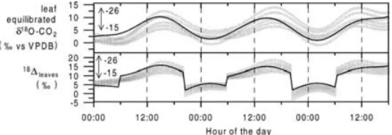
However, for the standard simulation we use the av- erage value ofεleaf= −7.4‰ to calculate the overall leaves, according to eq. (14) using δ¹⁸Oleaf, the iso- topic composition of leaf CO2in 93% isotopic equi-

Fig. 5. Model input data: dashed lines represent box 1, solid lines box 2 and dash-dotted lines box 3. NEE represents the CO2flux from box 2 to 3,F23(CO2). Note the different scales of the smoothed curves compared to Figs. 1 and 2. The model input curves represent the measured data of 29–31 July 1999; small discrepancies between data and curves are due to the smoothing procedure.

librium (Gillon and Yakir, 2000) with the measured bulk leaf water at ambient air temperature following Brenninkmeijer et al. (1983) and (ci−cc)/ce∼0.2 (Lloyd et al., 1992).

4.3. Model input data

A constant ²²²Rn soil exhalation rate of 10 Bq m⁻² s⁻¹ is used in the standard simulation. For box 3 the aircraft flasks were used to calculate the mean of this box for both, CO2mixing ratio andδ¹⁸O-CO2, with the heights at 100, 200 and 300 m. All measured data records used as input for the model are linearly inter- polated to the same time step (30 min), and afterwards a harmonic fit is applied to the data. The harmonic curve-fitting is done with the technique developed by the NOAA/CMDL Carbon Cycle Group and is docu- mented by Thoning et al. (1989). Figure 5 shows the

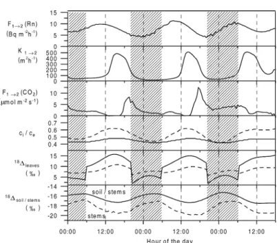
Fig. 6. Calculated model parameters: dashed lines represent box 1 and solid lines box 2. Note that during night (shaded area, by definition PAR<150µmol m⁻²s⁻¹) the assimilation flux is set to zero.

respective, smoothed model input records representing the measured data from 29 to 31 July 1999.

Figure 6 shows the calculated parameters of the model which determine the equation system (10)–

(13). The transport from box 1 to box 2 underlies a strong diurnal cycle as illustrated by the variability of F12(Rn) andK12. During night, vertical exchange is suppressed with an exchange coefficientK12of about 50 m²h⁻¹, which rapidly increases around noon up to values of about 500 m² h⁻¹. However, the CO2 flux from box 1 to box 2 calculated by eq. (9) shows a different behaviour. Despite an increasing exchange coefficientK12around noon, the CO2flux from box 1 to box 2 is nearly zero. This is due to the very small vertical CO2gradient between the mean CO2mixing ratios of both boxes. This gradient approaches zero and even becomes slightly positive (box 2 higher than box 1, Fig. 5). Therefore, in the model a minimum vertical gradient of 0.3 ppm (twice the standard reproducibility of the flask measurement) is fixed, whenever the mea- sured gradient falls below 0.3 ppm. With the build up of the vertical CO2gradient in the afternoon/evening, accompanied by still high exchange coefficientsK12, the CO2 transport from box 1 to box 2 increases to maximum values of about 7–15µmol m⁻²s⁻¹. Here, the gradient box model approach obviously reaches a

limit, because during strong vertical diffusion the flux is highly sensitive to very small gradients.

The ratio of sub-stomata cavity to ecosystem CO2

concentration,ci/ce, is calculated via eq. (15). Note here that only the day-time values are reasonable.

In reality, during night-time, sub-stomata cavity CO2

concentrations can reach values of several thousand ppm, due to missing assimilation activity and the dom- inating leaf respiration. Therefore, the model ignores the night-timeci/ceratios, and the assimilation flux is forced to be zero. Consequently, the calculation of the overall leaf discrimination against C¹⁶O¹⁸O,leaves, which depends onci/ce [eq. (14)], is also only rel- evant for the flux equation system (10)–(13) during day-time.ci/ceratios are modelled to vary between 0.4 and 0.6, values that are also observed elsewhere for C3 plants (Yakir and Sternberg, 2000). The overall leaf discrimination against C¹⁶O¹⁸O basically follows the diurnal cycle of the mean leaf water isotopic compo- sition in the respective box (Fig. 5). The diurnal cycle amplitudes range from about 7 to 10‰ for box 1 and from about 10 to 16‰ for box 2. Here comparison of leaveswith the discrimination against C¹⁶O¹⁸O by the soilsoiland the stemsstems, respectively, exhibits the potential ofδ¹⁸O-CO₂as a unique tracer: the im- print of the soils and stem respiration, respectively, on

Fig. 7. Model output of the standard simulation (solid lines): the gross fluxes (sum of box 1 and box 2), assimilation and respiration, along with the net exchange fluxF23(CO2) at the top of the canopy (original input function to the model, Fig. 5).

The dashed lines show the results of separated assimilation and respiration fluxes derived from the modified Lloyd and Taylor (1994) model, based on NEE measurements (Milyukova et al., 2002).

the ecosystemδ¹⁸O-CO2, is depleted by about 30‰, compared to the leaves. soil and stems show only a small temperature-driven variability, with a peak- to-peak amplitude of about 1–2‰, and mean values around−18‰ and−16‰, respectively.

5. Model results

5.1. Standard simulation

The model output gross fluxes of the standard sim- ulation are presented in Fig. 7 (solid lines). Assimi- lation fluxes are modelled to direct into the canopy, and they follow a diurnal cycle similar to PAR. Dur- ing day-time the model calculates assimilation fluxes resulting in maximum values between 40 and 50µmol m⁻²s⁻¹around noon. Simultaneously, to balance the mass flow, respiration is increasing up to about 30–

40µmol m⁻² s⁻¹. During night-time, when the as- similation is set to zero, the modelled respiration flux plus the CO2concentration gradient in time of each

-4 -3 -2 -1 0 1 2 3 4

C u m u la te d C O₂ flu x e s (m o l m^-2)

0 0 :0 0 1 2 :0 0 0 0 :0 0 1 2 :0 0 0 0 :0 0 1 2 :0 0

H o u r o f th e d a y

-4 -3 -2 -1 0 1 2 3 4 re s p ira tio n

a ss im ila tio n

N E E

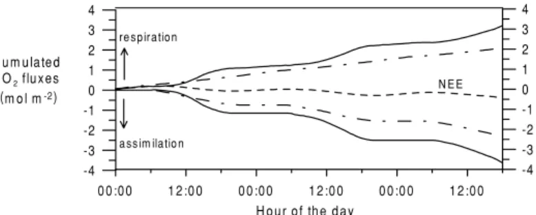
Fig. 8. Cumulated CO2fluxes. Standard simulation (solid lines), Lloyd and Taylor (1994) model (dash-dotted lines), along with the net ecosystem exchange (NEE) flux at the top of the canopy (dashed line).

box (CO2storage) is identical to the measured values of the eddy covariance measurements, which is a sim- ple consequence of the conservation of mass in the model equations. Figure 8 (solid lines) presents the cumulated gross fluxes during the model run of 72 h.

The one-dimensional (1-D) box model predicts cumu- lated assimilation fluxes of 3.6 mol m⁻² after 72 h.

By combination of transport and vegetation isotope exchange processes, the 1-D box model is able to sep- arate between assimilation and respiration fluxes. This appears to be trivial, and of course there is no reason to wonder about assimilation being a sink flux to the at- mosphere. However, this is the first approach that uses the¹⁸O interaction between CO2and H2O in a closed process/transport model, resulting in reasonable flux numbers.

5.2. Sensitivity runs

Assessment of the 1-D isotopic box model out- put requires a study of the sensitivity on the relevant

parameters controlling the respective processes. In principle, the model depends on the parameterisation of (1) the transport, (2) the isotopic composition of the interacting reservoirs and (3) the associated fraction- ations and discriminations.

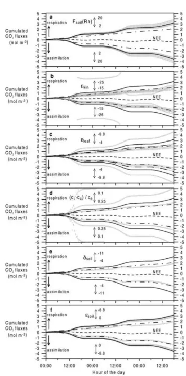
5.2.1. ²²²Rn transport calibration. The only vari- able that can change the model transport patterns between the bottom canopy boxes is the²²²Rn soil exhalation flux. Variation in the atmospheric CO2mix- ing ratio and²²²Rn activity vertical gradients within the measurement uncertainties does not significantly change the model transport patterns. In the model, the

222Rn soil flux is assumed to be constant in time and space. As the soil exhalation transect measurements show large spatial variation, correlated to soil water content (Levin et al., 2002), the mean value of 10 Bq m⁻² h⁻¹ used in the standard simulation needs not to be the actual soil²²²Rn influx to box 1. Further- more, the spatial heterogeneity of the soil²²²Rn flux leads to changing influxes to box 1, due to potentially changing footprint areas around the tower measure- ment site when the wind direction changes. The soil type directly below the tower showed a mean soil flux of 4.6±0.9 Bq m⁻²h⁻¹, whereas the overall soil type weighted footprint mean is 24.0±9.7 Bq m⁻² h⁻¹ in July 1999. Therefore, the model was tested for its sensitivity to the soil influxF_soil(Rn) in eq. (4) for a range from 2 to 20 Bq m⁻²h⁻¹, assumed to be relevant for the tower measurement site. Figure 9a presents the results of this test via the modelled cumulated gross fluxes. Variation ofFsoil(Rn) between 2 and 20 Bq m⁻² h⁻¹leads to deviations from the standard simulation between−8% and+16% for the resulting cumula- tive gross fluxes. LowerFsoil(Rn) leads to lower gross assimilation fluxes of the system. This is due to the changing intra-canopy transport parameterisation [eq.

(4)], i.e. a lower Fsoil(Rn) yields a lower exchange coefficient K12 which again decreases the CO2 flux from box 1 to box 2,F12(CO2) [eq. (9)]. This causes a higher assimilation flux in box 1 and a lower assimi- lation flux in box 2. As the assimilation activity of the system is controlled by box 2, the overall assimilation flux is decreasing.

5.2.2. Variations of isotopic composition and dis- criminations. The model is largely driven by the re- spective¹⁸O isotopic compositions of the CO2 and H2O reservoirs. Here it is assumed that the flask mea- surements deliver a precise characterisation of the CO2

mixing ratio and isotopic composition of the respective box because the model sensitivity tests within the mea- surement uncertainties showed no significant devia-

tions from the standard simulation. Within the equa- tion system (10)–(13) the sensitive terms are then given by the¹⁸O isotopic composition of leaves and soil, re- spectively. Together with the parameterisation of the associated fractionation and discriminations, sensitiv- ity is tested for the overall leaf discrimination and the overall soil “discrimination”.

5.2.2.1. Overall leaf discrimination,leaves: The overall leaf discrimination, leaves, is itself a func- tion of (1) theδ¹⁸O isotopic composition of leaf water, δleaf, (2) the¹⁸O-CO₂diffusion fractionation from the ecosystem air to the site of carboxylation,εleaf, and (3) the parameterisation of the chloroplast CO2concen- tration,cc. Therefore, the model sensitivity on these terms is investigated. Exemplary, the basic answer of leaveson varying parameterisations is shown for box 2 and the overall model sensitivity is presented via the cumulated gross fluxes.

δ¹⁸O isotopic composition of leaf water,δlea f: The leaf water isotopic compositions used in the model, are mean values of the measured bulk leaf water that were attributed to the respective box. One can easily imagine that these values need not to be representative for all leaves in the footprint that interacted with the observed CO2. This spatial heterogeneity in the signal is a serious problem. Furthermore, the isotopic compo- sition of the leaf water is also expected to be enriched at the site of evaporation, and huge gradients ofδ¹⁸O are observed within the leaf itself (Bariac et al., 1990).

Consequently, the measurement of the bulk leaf water may underestimate the enrichment of the interacting leaf waterδ¹⁸O.

An alternative approach to derive the leaf-water δ¹⁸O is to apply the steady-state leaf transpiration model of Craig and Gordon (1965). The Craig and Gordon model calculates the isotopic composition of leaf water according to:

δleaf=εliq−vap+(1−rh)(δroot−εkin)+rhδvap. (17) In our study the relative humidity, rh, is assumed to be the measured relative humidity within the ecosys- tem.δroot, representing the δ¹⁸O of root H₂O taken up from the soil water, was also measured, as well as the δ¹⁸O of water vapour outside the leaf,δvap. The equilibrium fractionation of H218O for the liquid–

vapour phase transition εliq−vap is well known and varies with temperature (Majoube, 1971). Only the kinetic fractionation of H218O for the diffusion of wa- ter vapour across the sub-stomata cavity via the leaf boundary layer to the ecosystem air,εkin, is not well

Fig. 9. Sensitivity runs for varying the soil exhalation rateFsoil(Rn) (a), the kinetic fractionation of H218O for the diffusion of water vapour,εkin(b), the effective diffusion fractionation of C¹⁶O¹⁸O from the ecosystem to the site of carboxylation, εleaf (the run using the parameterisedεleaf (see text) is represented by the long-dashed line) (c), the parameterisation of (ci−cc)/ce(d), the soil waterδ¹⁸O-H2O composition,δ^soil(e), and the effective soil fractionation against C¹⁶O¹⁸O during diffusion through the soil to the ecosystem atmosphere,εsoil(f). NEE derived gross fluxes following the Lloyd and Taylor model (Milyukova et al., 2002) are given as the dash-dotted lines, along with the NEE at the top of the canopy (dashed lines).

The standard simulation is represented by the solid lines.