Long-Term Asset Allocation

(1)

DISSERTATION

zur Erlangung des Grades eines

Doktors der Wirtschaftswissenschaft (Dr. rer. pol.)

eingereicht bei der

Wirtschaftswissenschaftlichen Fakult¨ at der Universit¨ at Regensburg

von

Dipl.-Math. Oec. Tim Koniarski

Berichterstatter

Prof. Dr. Steffen Sebastian Prof. Dr. Rolf Tschernig

Tag der Disputation

6. Februar 2014

(2)

1 Introduction 1 2 Inflation-Protecting Asset Allocation: A Downside Risk Analysis 5

2.1 Introduction . . . 6

2.2 Methodology . . . 10

2.2.1 Modeling Asset Return Dynamics . . . 10

2.2.2 The Concept of Lower Partial Moments . . . 12

2.2.3 The Portfolio Choice Problem . . . 13

2.3 Empirical Analysis . . . 14

2.3.1 Data . . . 14

2.3.2 VAR Estimation Results . . . 18

2.3.3 Inflation Protection of Individual Assets . . . 21

2.3.4 Inflation-Protecting Asset Allocation . . . 24

2.4 Conclusion . . . 29

3 Modeling Asset Price Dynamics under a Multivariate Cointegra- tion Framework 31 3.1 Introduction . . . 32

3.2.1 VAR Specification . . . 35

3.2.2 VEC Specification . . . 36

3.2.3 Horizon-Dependent Variance-Covariance . . . 37

3.2.4 Portfolio Choice Problem . . . 39

3.3.1 Data and Time Series Properties . . . 41

(3)

3.3.2 Estimation Results . . . 46

3.3.3 Long Horizon Effects . . . 54

3.3.4 Asset Allocation Decisions . . . 63

3.A Appendix . . . 70

3.A.1 Bootstrap Method . . . 70

3.A.2 Model Selection . . . 71

4 Do Stock Prices and Cash Flows Drift Apart? The Influence of Macroeconomic Proxies 72 4.1 Introduction . . . 73

4.2.1 The Econometric Model . . . 76

4.2.2 Hypotheses Testing . . . 77

4.2.3 Long-Run Analyses . . . 79

4.2.4 Returns . . . 80

4.3.1 Data and Time Series Properties . . . 81

4.3.2 Cointegration Rank Analysis . . . 87

4.3.3 Restriction Tests . . . 90

4.3.4 Testing the Financial Ratios . . . 93

4.3.5 Level Effects . . . 95

4.3.6 Horizon-Dependent Analysis . . . 97

4.A Appendix . . . 103

4.A.1 Model Selection . . . 103

4.A.2 Univariate Stationarity of the Financial Ratios . . . 104

4.A.3 Stability of the Long-Run Matrices across the Models . . . 105

4.A.4 Bootstrap Method . . . 107

Bibliography 108

(4)

2.1 Correlations between Asset Returns and Inflation . . . 22

4.1 Level Variables . . . 85

4.2 Differenced Variables . . . 86

4.3 Impulse Response Functions . . . 98

4.4 Impulse Response Functions of Returns . . . 100

(5)

2.1 Descriptive Statistics . . . 17

2.2 VAR Estimation Results . . . 19

2.3 Lower Partial Moments of the Asset Returns . . . 23

2.4 Minimum Semivariance Portfolios with Real Return Target of 0% . . 25

2.5 Minimum Semivariance Portfolios with Positive Real Return Targets . 27 3.1 Abbreviationsg . . . 42

3.3 Simultaneous and Lagged Correlations . . . 44

3.4 Unit Root and Cointegration Rank Test . . . 45

3.5 VAR Parameter Estimatesg . . . 47

3.6 VEC Parameter Estimatesg . . . 50

3.7 Term Structure of Risk and Correlationsg. . . 55

3.8 Variance Decomposition for Treasury Bills . . . 57

3.9 Variance Decomposition for Stock Returns . . . 58

3.10 Variance Decomposition for Bond Returns . . . 61

3.11 Global Minimum Variance Portfoliosg . . . 64

3.12 Optimal Portfolio Holdings for γ = 20 . . . 66

3.13 Lag Length Selection . . . 71

4.1 Univariate Stationarity . . . 82

4.3 Cointegration Rank . . . 89

4.4 β Restriction Tests . . . 91

4.5 αRestriction Tests . . . 92

(6)

4.6 Financial Ratio Stationarity Tests . . . 94

4.7 Π_r Matrix of Model M₆ and r= 4 . . . 96

4.8 Lag Length Selection and Cointegration Rank Stability . . . 103

4.9 Univariate Stationarity of Financial Ratios . . . 104

4.10 Stability Analysis of the Long-Run Matrices . . . 106

(7)

Introduction

Individual as well as institutional investors face the decision of how to allocate assets in their portfolios. In general, it is distinguished between strategic and tactical asset allocation. While strategic asset allocation concentrates on the allocation and diversification of a portfolio among major asset classes such as cash, bonds, stocks and real estate, tactical asset allocation is a dynamic adjustment of the strategic asset allocation weights with the intent to add value due to a changing fundamental market environment. This thesis focuses on strategic asset allocation and determines optimal portfolios for investors with specific objectives (inflation-hedging) and/or with a focus on long-term investments.

The era of modern portfolio theory starts with the seminal work of Markowitz (1952), which introduces the famous mean-variance optimization framework, an approach that determines optimal portfolios which exhibit minimum risk measured by the variance for a given required return. Although Markowitz optimization is still widely used in academia and in practice, it has the limitation that it is static, i.e.

only a one-period investment horizon is considered, which is unrealistic for long-term investors. Due to the fact that the assets’ term structure of risk and asset correlations vary substantially over the investment horizon, optimal horizon-dependent asset allocations are also time-varying (Campbell and Viceira, 2005). To take into account this time variation in the term structure of risk, the asset allocation literature is currently focusing on more sophisticated portfolio approaches. The complex dynamics of expected returns and risk are usually captured by stationary vector

(8)

autoregressive (VAR) models, which typically contain the returns of the assets analyzed and some so-called state variables, which are used to predict these returns.

Such VAR models are also used in the following three self-contained chapters/essays of this thesis, but several contributions to the asset allocation literature are made as well.

In the essay ’Inflation-Protecting Asset Allocation: A Downside Risk Analysis’

(Chapter 2), written in cooperation with Steffen Sebastian, we are the first to apply the VAR approach to bootstrap multi-period asset returns, which maintains the asymmetric asset return distributions. Additionally, we determine the inflation- protecting abilities of cash, bonds, stocks and real estate and optimal horizon- dependent inflation-protecting asset allocations within a downside risk framework.

This downside risk analysis was inspired by two facts. First, previous studies only analyze correlation statistics between asset returns and the inflation rate to investigate the inflation-hedging qualities of the assets mentioned. However, correlation only measures the linear relation between the return and inflation. Thus, a positive correlation does not necessarily imply that the asset is a good inflation hedge, because the asset return could always be lower than the inflation rate despite the positive correlation. This issue has not been addressed in earlier studies and hence, we compare these correlations to lower partial moments (LPM) which measure the risk of the asset to fall below the inflation rate. Second, we argue that the most widely used risk measure in the asset allocation context, the variance, does not adequately represent the risk perception of investors and downside risk measures are more suitable to investors’ risk understanding and in the presence of asymmetric return distributions. Markowitz (1959) already pointed out the advantages of downside risk measures compared to the variance, but it was not possible to handle those risk measures at that time due to their computational complexity.

In the essay ’Modeling Asset Price Dynamics under a Multivariate Cointegration Framework’ (Chapter 3), written in cooperation with Benedikt Fleischmann, we argue that the traditional VAR approach to modeling long-run asset price dynamics ignores common long-run relations between the assets and the state variables. In the presence of so-called cointegration relations, deviations in the long-term comovement

(9)

cointegration relations among the assets and state variables, we capture the asset price dynamics using a vector error correction (VEC) model, which is an extension of the stationary VAR model. We, then, make several comparisons between the VEC and the stationary VAR approach, where both models include T-bills, stocks and bonds and the same set of state variables that have been shown to predict returns (dividend-price ratio, term spread and inflation). These comparisons include the modeled short and long-run behavior, the term structure of risk and the resulting optimal portfolio choice.

In the essay ’Do Stock Prices and Cash Flows Drift Apart? The Influence of Macroeconomic Proxies’ (Chapter 4), written in cooperation with Benedikt Fleisch- mann, we examine the validity of cointegration between stock prices and cash flows and analyze the additional influence of macroeconomic proxies within a cointegrated VAR framework. This paper is motivated by the fact that the often used state variables in the traditional VAR approach such as the dividend-price or the earnings- price ratio are assumed to be stationary. Since these one-for-one cointegration relations are empirically doubtful and non-stationarity would lead to invalid conclusions about the return forecastability, we investigate possible macroeconomic influences (inflation, short-term interest rates, government and corporate bond yields) which can cause the breakdown of these relations. Thus, although we do not determine optimal asset allocations, this paper is still relevant for the asset allocation literature as return predictions are of significant importance for portfolio choices.

(10)

Research Questions

This section gives a short overview of the research questions examined in each essay of this thesis:

Chapter 2: Inflation-Protecting Asset Allocation: A Downside Risk Analysis

• Do correlations and LPMs provide the same results with respect to the inflation- protecting abilities of cash, bonds, stocks and real estate?

• What are optimal horizon-dependent inflation-protecting asset allocations within the downside risk framework?

• How do optimal allocations differ for investors that require a positive real return?

Chapter 3: Modeling Asset Price Dynamics under a Multivariate Coin- tegration Framework

• Are there differences of the VEC compared to the VAR model with respect to the predictability of cash, stocks and bonds?

• What are the differences in the term structure of risk modeled by the two approaches and what are the sources of these differences?

• How do the optimal portfolio choices suggested by the two models differ?

Chapter 4: Do Stock Prices and Cash Flows Drift Apart? The Influ- ence of Macroeconomic Proxies

• Is the assumption of stationarity of the dividend-price ratio and the earnings- price ratio valid in the multivariate cointegration framework?

• Is the assumption of stationarity of other financial ratios, which are additionally used in the predictability literature, valid in the multivariate cointegration framework?

• How do the macroeconomic variables influence stock prices and cash flows and what are the resulting consequences on total stock returns?

(11)

Inflation-Protecting Asset

Allocation: A Downside Risk Analysis

This paper is the result of a joint project with Steffen Sebastian.

Abstract

This paper studies the ability of cash, bonds, stocks and direct real estate to hedge inflation and optimal inflation-protecting asset allocations within a downside risk framework. Using a VAR model to capture predictable price dynamics, we find that the inflation-hedging properties of assets substantially change over the investment horizon. Cash is clearly the best hedge against inflation in the short run. However, as the investment horizon increases, bonds, stocks, and real estate become the more attractive options, with real estate exhibiting the best inflation protection qualities on a medium and long-term basis. While cash plays the most important role in short-term portfolios, the weights of the inflation-protecting portfolios shift to real estate, stocks and bonds as the investment horizon increases.

(12)

2.1 Introduction

In the United States as well as Europe interest rates are at an all-time low level, resulting in a continuous rise of the money volume. Furthermore, many developed countries are choosing to inject liquidity into their markets in order to stimulate the economy. However, there is a real danger that these monetary policies pave the way to rising inflation bringing the concerns of inflation back to investors’ minds. Such fears are not restricted to institutional investors, whose liabilities are often linked to consumer prices or wage levels. They can also affect private investors, who seek to preserve their real capital, as well. Thus, the debate over inflation-protecting properties of assets and how investors can obtain optimal asset allocations to hedge against inflation has been revived.

Since many investors make long-term investments and it is well documented that the term structure of asset risk, asset correlations and the inflation rate can vary over time, the inflation-protecting properties of assets may also change essentially with the investment horizon.

In this paper, we therefore focus on inflation protection not only on short, but on various investment horizons up to 30 years. We consider an investor able to invest in cash, bonds, stocks and direct commercial real estate who seeks inflation protection.

In contrast to studies that cover primarily asset and liability management (ALM) (see e.g. Amenc, Martellini, Milhau, and Ziemann, 2009), we assume that the investor’s sole objective is to protect her assets against inflation, and that she has no liabilities subject to inflation risk. Using a vector autoregressive (VAR) model to capture predictable asset price and inflation dynamics, we first investigate the time-dependent correlations between the assets and inflation. This is the standard procedure for examining the horizon-dependent inflation-hedging properties of assets (Hoevenaars, Molenaar, Schotman, and Steenkamp, 2008; Amenc, Martellini, Mil- hau, and Ziemann, 2009; Briere and Signori, 2012). Note, however, that analyzing only correlations can be misleading, because a high positive correlation between an asset class and inflation does not necessarily imply a good inflation-protection ability. The asset return could still be lower than the inflation rate despite the positive correlation. To gain further insight into the inflation-hedging abilities of the assets

(13)

analyzed, we examine the downside risk measures over various investment horizons based on asset returns generated by the VAR model. In particular, our analysis focuses on lower partial moments (LPM) to measure the risk of assets to fall below the inflation rate. LPMs are also useful for studying optimal inflation-protecting asset allocations over various investment horizons, because they can account for downside return deviations as well as asymmetric return distributions, which are observed empirically. We also argue that the variance, the most commonly used risk measure, does not adequately represent investors’ risk perception, because it captures both negative and positive deviations from the mean. Since we consider investors with inflation-hedging motives but no liabilities, it is more suitable to focus only on the negative deviations of a specified target return. Due to concerns about using the variance as risk measure and to account for any the asymmetric asset returns, we apply a downside risk approach instead of the traditional Markowitz (1952) mean-variance approach to determine optimal portfolios.

Comparing the correlation analysis with the LPM analysis, we obtain different results for the inflation-protecting properties of assets and conclude that high correlations do not necessarily imply low LPMs. While the correlation analysis detects cash to be the best inflation hedge over all horizons (which is in line with Hoevenaars, Molenaar, Schotman, and Steenkamp (2008) and Amenc, Martellini, Milhau, and Ziemann (2009)), by analyzing LPMs, however, we find that the inflation-protecting potential of cash, stocks, bonds, and real estate changes substantially over the investment horizon. In the short term, cash is clearly a superior hedge. As the investment horizon increases, bonds, stocks, and real estate become the more attractive options.

In fact, in contrast to the correlation results, they are better inflation protectors than cash in the long run, with real estate ultimately exhibiting the best inflation protection qualities for medium and long-term horizons. Bonds outperform equities with respect to inflation protection for medium horizons, but we obtain contrary results in the long run. These findings, consequently, also affect horizon-dependent optimal asset allocations. While cash is the only relevant asset for short-term optimal inflation-hedging portfolios, real estate plays the most important role in medium and long-term portfolios. In our asset allocation analysis, we consider not only an investor desiring to preserve capital, but also an investor with a more performance-

(14)

oriented goal. Increasing the target return, i.e. considering an investor who aims to achieve a premium in excess of the inflation rate, we find that larger weight is assigned to assets that are riskier than cash. Over a medium and long-term basis, the largest proportion of investor capital should be invested in real estate. Equities also become highly attractive for investors who require a positive real return in the long run.

This paper contributes to the existing literature in two areas: inflation-hedging and strategic asset allocation. A number of studies have investigated the inflation- protecting abilities of various asset classes by employing correlation statistics between assets and inflation or regression models such as Fama and Schwert (1977). A detailed review of these studies is given by Atti´e and Roache (2009). Most inflation- hedging research has focused only on the relationship between an asset class and inflation for short-term investment horizons. Using a VAR framework, Campbell and Viceira (2005) demonstrate that the risk of T-bills, stocks and bonds, as well as the correlations between these assets, can vary considerably over time, which implies changes in the optimal asset allocation. These effects also have an essential impact on horizon-dependent inflation-protecting abilities of assets and the optimal inflation- hedging asset allocations. This VAR approach to analyzing the term structure of risk and horizon-dependent portfolios was first used in a classical asset allocation context with no reference to inflation-hedging. Fugazza, Guidolin, and Nicodano (2007) and Fugazza, Guidolin, and Nicodano (2009) extend the model of Campbell and Viceira (2005) by including European and U.S. property shares, respectively.

MacKinnon and Zaman (2009) include U.S. direct real estate and REIT investments in addition to cash, bonds and stocks, whereas Rehring (2012) analyzes the role of direct real estate in a horizon-dependent mixed-asset portfolio for the U.K. market.

Hoevenaars, Molenaar, Schotman, and Steenkamp (2008) and Amenc, Martellini, and Ziemann (2009) are the first to investigate optimal horizon-dependent portfolios with respect to inflation-hedging. Using a VAR methodology¹, they extend the model with alternative asset classes and investigate optimal portfolios for investors with liabilities subject to inflation risk. More recently, Briere and Signori (2012)

1Amenc, Martellini, and Ziemann (2009) use a cointegrated VAR model or vector error correction model, which allows for cointegration relations among the included variables.

(15)

find that inflation-hedging portfolios can be influenced by macroeconomic regimes.

In contrast to previous studies, they do not apply the traditional mean-variance framework to derive optimal allocations of several listed assets, but they instead op- timize portfolios with respect to inflation shortfall probabilities. Note, however, that their portfolio optimization focuses only on shortfall probabilities while ignoring the expected shortfall, which is an issue of great interest to investors. Their portfolio model also does not consider co-movements of individual assets. This appears restrictive in the presence of high correlations between asset returns. In this paper, we use the semivariance as downside risk measure for portfolio optimization and we account not only for the shortfall probability, but also for the amount of shortfall with an inflation target as well as co-movements among assets. Several studies have used semivariance approaches in a portfolio context (see e.g. Nawrocki (1999) for an overview; more recent articles are Kroencke and Schindler (2010) and Cumova and Nawrocki (2011)). But to the best of our knowledge, none has examined horizon- dependent asset allocations or inflation-hedging properties of assets. To investigate various investment horizons in a downside risk framework, it is necessary to simulate multi-period returns of the assets analyzed. In contrast to previous studies (such as Amenc, Martellini, and Ziemann (2009) or Briere and Signori (2012)), we do not simulate returns by means of a multivariate normal distribution. This procedure assumes that the asset returns exhibit no asymmetric behavior. However, it is widely accepted and we also find that asset returns are asymmetric and not normally distributed. Taking this into account, we apply a bootstrap resampling method for multi-period return generation. Thus, we believe this paper is the first to study the inflation-protecting abilities of cash, bonds, stocks and direct real estate as well as the optimal inflation-protecting portfolios over various investment horizons within an LPM framework.

The remainder of the paper is organized as follows. After introducing the applied methodology in the next section, we present our dataset and the results of our empirical analysis in Section 2.3. Section 2.4 summarizes the main findings and concludes.

(16)

2.2 Methodology

In this section we describe the VAR model used to capture return and inflation dynamics and to generate multi-period returns. We also present the risk measures that are applied to analyze the inflation-protecting properties of cash, bonds, stocks and real estate. Finally, the downside risk optimization problem to calculate optimal inflation-protecting asset allocations is given.

2.2.1 Modeling Asset Return Dynamics

The VAR model is a popular framework for modeling long-run asset price dynamics.² Hence, we follow this approach and capture the return dynamics of cash, bonds, stocks and real estate as well as the inflation rate by a first-order VAR model.

Let

z_t= (r_ca,t, r_bo,t, r_st,t, r_re,t, inf l_t,s_t)⁰ (2.1) contain the log returns of cash (r_ca,t), bonds (r_bo,t), stocks (r_st,t) and real estate (r_re,t), the log inflation rate³ (inf l_t) and three other state variables (the log of the dividend price ratio, the term spread and the cap rate), which are stacked in s_tand help to forecast asset returns. Thus, z_t is a (8×1) vector. We assume the return process is truly generated by the VAR(1) model:

z_t+1 =µ+Φz_t+u_t+1, (2.2)

whereµ is the intercept vector of dimension (8×1) andΦis the (8×8) coefficient matrix. The vector u_t+1 of dimension (8×1) contains the disturbances of the VAR model which we assume to beIIDwith zero means and a variance-covariance matrix Σ.

2Authors using the VAR methodology to account for predictability and the horizon effects of asset returns are, e.g.: Campbell and Shiller (1988a,b); Campbell (1991); Campbell and Ammer (1993); Kandel and Stambaugh (1996); Barberies (2000); Campbell, Chan, and Viceira (2003);

Campbell and Viceira (2005); Hoevenaars, Molenaar, Schotman, and Steenkamp (2008); Jurek and Viceira (2011).

3The log inflation rate is the difference between the logs of the price levels.

(17)

We first examine the inflation-protecting abilities of the assets analyzed by considering horizon-dependent correlations between the assets and inflation. These correlations are based on the conditional k-period variance-covariance matrix implied by the VAR model (see e.g. Campbell and Viceira, 2004):

V ar_t(z_t+1+· · ·+z_t+k) =Σ+ (I+Φ)Σ(I+Φ)⁰ + I+Φ+Φ²

Σ I+Φ+Φ²⁰

+. . . (2.3) + I+Φ+· · ·+Φ^k−1

Σ I+Φ+· · ·+Φ^k−1⁰ , We then use the VAR model in equation (2.2) to generate k-period returns for cash, bonds, stocks and real estate and the inflation rate depending on the investment horizon. In contrast to previous studies (see e.g. Amenc, Martellini, and Ziemann, 2009; Briere and Signori, 2012), we do not simulate returns by drawing variables from a multivariate standard normal distribution. This procedure assumes that the residuals of the VAR model, and also the asset returns, are normally distributed and, therefore, exhibit no asymmetric behavior. However, it is widely accepted that asset returns are usually asymmetric. Taking into account this fact, we apply a bootstrap resampling method to generate multi-period returns following Benkwitz, L¨utkepohl, and Wolters (2001) and L¨utkepohl (2005), which consists of the following steps:

1. Calculate centered residuals ˆu₁ −u, ...,¯ uˆ_T −u, where ˆ¯ u₁, ...,uˆ_T are the estimated residuals and ¯u contains the eight usual means of the eight residual series.

2. Draw randomly with replacement from the centered residuals to obtain bootstrap residuals ^∗₁, ...,^∗_T.

3. Recursively calculate the bootstrap time series for the VAR as

z^∗_t+1 =µ+Φz^∗_t +^∗_t, t= 1, ..., T, (2.4) wherez^∗₁ =z1 holds for each generated series.

4. Calculate one-period log returns z^∗₁, ...,z^∗_k by the VAR equation in (2.2) and obtain the k-period log returns by z^∗₁+· · ·+z^∗_k.

(18)

5. Repeat these steps 10,000 times.

After bootstrapping these returns, we adjust the k-period returns by transaction costs. This is important because we include direct real estate into the analysis and in comparison to the other assets analyzed, the transaction costs of real estate are much higher and make real estate attractive only for longer investment horizons (details of the transaction cost adjustments are given in the next section). These generated multi-period returns are not only used to analyze the inflation-protecting properties of the asset classes with respect to LPMs over various investment horizons, but also to construct minimum downside risk portfolios for different investment horizons.⁴

2.2.2 The Concept of Lower Partial Moments

In addition to the correlations implied by the VAR model, we also want to measure the risk of the assets to fall below the inflation rate. LPMs, a concept first intro- duced by Bawa (1975) and Fishburn (1977), are quite useful in this regard because they focus on the downside (left-side) of the return distribution. Moreover, LPMs are also an adequate risk measure for our portfolio analysis. In contrast to the variance, LPMs only capture negative return deviations of a specified target, which is more intuitive since returns above the target are considered desirable and non-risky.

Furthermore, asset returns are empirically observed to be non-normally distributed, a feature that LPMs can also handle very efficiently.

Generally, the LPM of order n is defined as:

LPM_n(τ) = Z τ

−∞

(τ −r_i)ⁿf(r_i)dr_i, (2.5) whereτ is the target rate,r_i is the return of asset iandf(r_i) is the density function of the ith asset return. Observing T returns of asset i, the discrete version of the LPM of order n is given by:

LPM_n(τ) = 1 T

T

X

t=1

[max(0,(τ −r_it))]ⁿ. (2.6)

4The bootstrap is theoretically justified as the statistics of interest have a normal limiting distribution (Horowitz, 2001; Barrett and Donald, 2003; L¨utkepohl, 2005).

(19)

The order n of the LPM can be interpreted as a risk aversion parameter. Higher values ofn penalize deviations below the target more strongly. This analysis focuses on three classes of LPMs: the shortfall probability (n = 0), the expected shortfall (n= 1) and the semivariance (n = 2).

In the portfolio context, similarly to the traditional mean-variance framework, co- movements of the LPMs of individual asset returns need to be taken into account.

These co-movements are captured by co-lower partial moments (CLPM). There are several definitions for CLPMs between two assets. Nawrocki (1991) presents an asymmetric as well as a symmetric CLPM algorithm. Comparing both concepts empirically, Nawrocki (1991) recommends the usage of the symmetric measure. The most recent approach for measuring the CLPM between two assets was developed by Estrada (2008). In his heuristic framework the semivariance between assetiand asset j is calculated as:

CLPM_ij(τ) = 1 T

T

X

t=1

[max(0,(τ−r_it))·max(0,(τ −r_jt))]. (2.7) In contrast to the symmetric CLPM of Nawrocki (1991), Estrada’s CLPM definition considers only downside co-movements, which induces us to apply his approach in this paper.

2.2.3 The Portfolio Choice Problem

There is a great deal of extant literature on long-horizon asset allocation and inflation-hedging in the portfolio context. However, most of the papers use a mean- variance framework with variance as the risk measure to be minimized. Due to concerns about the efficacy of this method and in order to consider non-normally distributed returns, we apply a downside risk framework in our analysis. Markowitz (1959) discussed the advantages using the downside risk measure, but he did not apply this approach due to its computational complexity. The downside risk portfolio choice problem is quite similar to the traditional Markowitz approach, as we can replace the variance matrix by the semivariance of the portfolio and minimize the downside risk measure, which is suggested by Harlow and Rao (1989) and Harlow (1991). In their approach, however, co-movements between assets are disregarded,

(20)

which is restrictive in the presence of high correlations between the LPMs of the assets. Thus, taking into account co-movements, we approximate the semivariance according to Estrada (2008) and consider the following minimum semivariance portfolio choice problem:

minw LPM_2,p =

4

X

i=1 4

X

j=1

w_iw_jCLPM_ij(τ) (2.8) subject to

4

X

i=1

w_i = 1

w_i ≥0, i= 1, ...,4,

where the vectorw= (w₁, w₂, w₃, w₄) contains the weights of the four assets analyzed in the minimum downside risk portfolio.

In the empirical part of this study, we calculate the semivariance using k-period real asset returns. At first, we assume an investor who seeks to hedge inflation and we calculate minimum semivariance portfolios with the target rate set to 0 (i.e., we minimize the risk of achieving a negative real return). Afterward, we consider a more ambitious investor with respect to the required real return and we determine portfolios with annualized target rates ranging from 1% to 3%.⁵

2.3 Empirical Analysis

This section discusses the results of our empirical analysis. After introducing the dataset, we present the estimated VAR model capturing the asset return and inflation dynamics. Then, the inflation-protecting properties of the assets are analyzed and inflation-hedging portfolios described.

2.3.1 Data

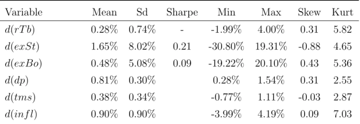
Our empirical application is based on the four most widely used asset classes in the United States: cash, bonds, stocks and direct real estate. We use quarterly data

5Throughout the remainder of this paper, we use the term ”target rate/return” rather than

(21)

from 1978:Q1 to 2010:Q4.⁶ Cash is represented by the 90-day Treasury bill rate.

Bonds are the long-term U.S. government bond returns and stock returns (including dividends) are calculated using the S&P 500 index. The data concerning these assets stem from Goyal and Welch (2008).⁷ Direct real estate data is obtained from the NCREIF Property Index (NPI).⁸

Real estate returns are determined by appraisal-based capital and income indices.

Appraisal-based indices/returns cannot be directly compared to those of liquid assets such as stocks, because they are smoothed and lagged with respect to market movements. Moreover, the systematic risk of appraisal-based returns is lower and less volatile than true real estate market returns (see e.g. Geltner, N. G. Miller, and Eichholtz, 2007, Chap. 25). This underestimation of risk can make appraisal-based returns more attractive than they actually are and incomparable to returns of liquid and more volatile assets. Therefore, we unsmooth the appraisal-based returns following the approach of Geltner (1993). The appraisal-based log real capital returns, c^∗_t, are unsmoothed by:

c_t= c^∗_t −(1−ω)c^∗_t−1

ω , (2.9)

where ct is the log real capital return and ω is the smoothing parameter. This parameter is determined by ω = 1/( ¯L+ 1), where ¯L is the average number of lags.

Since we use quarterly data, we have ¯L= 4 and unsmooth the log real capital returns withω = 0.2 (as suggested by Geltner, N. G. Miller, and Eichholtz, 2007, Chap. 25).

Afterwards, the unsmoothed log real capital returns are retransformed to nominal capital returns (U CR_t) and we use U CR_t to calculate an unsmoothed capital value index (U CVt). Multiplying the income return (IRt) with the original capital value index (CV_t), we obtain an income series (In_t) and the unsmoothed income returns (U IRt=Int/U CVt), out of which we finally determine the unsmoothed total returns by summing up the unsmoothed income and capital returns (U IR_t+U CR_t).

6The beginning of the sample was chosen according to the availability of direct real estate data.

7We would like to thank Amit Goyal for providing an updated version of this data which is available on his website: http://www.hec.unil.ch/agoyal/.

8We would also like to thank NCREIF for providing the data.

(22)

We further use some common state variables that have been shown to predict returns: the dividend-price ratio, the term spread and the cap rate, which reflects the real estate market yield and is determined by In_t/U CV_t. The dividend-price ratio is often used as a predictor of future aggregate stock returns (Campbell and Shiller, 1988a,b; Fama and French, 1988; Hodrick, 1992; Goetzmann and Jorion, 1993). The term spread is a business cycle indicator and positively forecasts bond returns (Campbell and Vuolteenaho, 2004; Campbell and Viceira, 2005; Jurek and Viceira, 2011). Fu and Ng (2001) and Plazzi, Torous, and Valkanov (2010) find the cap rate to predict future direct real estate returns. Moreover, we include the inflation rate as a state variable to analyze the inflation-protecting properties of the asset classes and portfolios. With the exception of the cap rate, which is calculated by the NCREIF data, the data of the state variables is also obtained from Goyal and Welch (2008).

Table 2.1 provides an overview of the sample statistics of the variables used.

Cash has the lowest nominal return compared to the other asset classes.⁹ The most attractive asset class with respect to the return is stocks followed by real estate and bonds. The hierarchy of asset volatilities is the same as for returns. Cash has the lowest variability followed by bonds, real estate and stocks. Considering the skewness of the assets, we detect an asymmetric behavior of asset returns. While cash and bonds are positively skewed, stocks and real estate returns have a negative skewness.¹⁰ Moreover, the (excess) kurtosis of all assets is different from zero¹¹ and the asset returns do not follow a normal distribution as indicated by the Jarque-Bera test for normality. The test rejects the null of normality for cash and bonds on a 5% and for stocks and real estate on a 1% significance level.

9Hereinafter we write ”returns” and ”rates” instead of ”log returns” and ”log rates”.

10According to the D’Agostino test for skewness, the null of no skewness is rejected for stocks on a 5% significance level and for cash and real estate on a 10% significance level. The null is supported for bonds.

11According to the Anscombe-Glynn test for kurtosis, the null of no kurtosis is rejected for real estate on a 1% significance level and for bonds and stocks on a 5% significance level. The null is

(23)

Table2.1:DescriptiveStatistics MeanSdMinMaxSkewKurtJB-Test Returns Cash(rca)1.32%0.80%0.01%3.60%0.570.267.83* Bonds(rbo)2.36%6.05%-15.68%21.81%0.390.969.14* Stocks(rst)3.08%8.17%-25.57%19.33%-0.861.2325.53** Realestate(rre)2.59%8.15%-26.79%21.66%-0.561.5521.25** StateVariables Loginflation(infl)0.94%0.99%-3.99%4.19%-0.224.55119.83** Logtermspread(tms)0.49%0.37%-0.77%1.11%-0.640.229.61* Logdividendpriceratio(dp)-3.640.46-4.49-2.780.02-1.136.58* Logcaprate(cr)-3.990.16-4.46-3.73-0.850.2016.52** Notes:Thistablereportssummarystatisticsofthesamplefrom1978:Q1to2010:Q4.Meanlog returnsareadjustedbyonehalfofthevariancetoreflectlogmean(gross)returns.”Sd”denotes standarddeviation,”Min”denotesminimum,”Max”denotesmaximum,”Skew”denotesskewness, ”Kurt”denoteskurtosisand”JB-Test”denotestheteststatisticoftheJarque-Beratestfornormality. *and**indicatetherejectionofthenullhypothesisat5%and1%significancelevels,respectively.

(24)

2.3.2 VAR Estimation Results

We capture the predictable return and inflation dynamics by the VAR(1) model given in equation (2.2).¹² Table 2.2 presents the estimation results of the VAR model.

Panel A shows OLS estimates with bootstrapped standard errors in parentheses.

The bootstrap estimates are calculated from 10,000 paths under the assumption that the initial estimated VAR model truly generates the data process. The R² and F-statistics are given in the rightmost column. Panel B reports the covariance structure of the VAR residuals showing the standard deviations of the innovations on the main diagonal and the cross-correlations above the main diagonal.

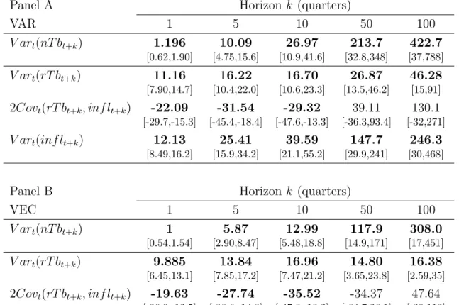
The first row in Panel A represents the prediction equation for cash, which is highly predictable according to the high R² of 89.39%. It shows that the own lag has a high positive influence on T-bills. The second and third rows correspond to bonds and stocks. These variables seem to be more difficult to predict, as they exhibit the lowest R²’s. However, bond returns are explained by T-bills, inflation and the term spread with positive slopes. In the stock equation the dividend-price ratio has a positive influence on equities. Obviously, real estate returns are easier to predict compared to stocks and bonds, as indicated by an R² of 35.72%. The cap rate helps to forecast real estate returns with a positive coefficient. The last four rows represent the state variable equations. The equations of the term spread, dividend-price ratio and cap rate reveal the persistent autoregressive behavior of these variables with high coefficients of their own lags. These results are consistent with previous studies such as Campbell and Viceira (2005), Fugazza, Guidolin, and Nicodano (2007) and Briere and Signori (2012).

Turning to the covariance structure of the innovations in Panel B, we see that unexpected inflation is positively correlated with shocks to cash and negatively correlated with shocks to bonds, stocks and real estate. The correlations of the residuals seem to imply that only cash is a good inflation hedge. However, although bonds, stocks and real estate are negatively correlated with inflation innovations, these asset classes may protect investors against inflation as the investment horizon increases.

12The lag length one is confirmed by the Schwarz information criterion.

(25)

Table2.2:VAREstimationResults PanelACoefficientsoftheLaggedVariablesR2 rca,trbo,trst,trre,tinflttmstdptcrt(F-stat.) rca,t+10.870.000.010.010.00-0.030.000.0089.39% (0.09)(0.00)(0.00)(0.00)(0.03)(0.14)(0.00)(0.00)(127.45) rbo,t+15.34-0.04-0.070.010.839.46-0.05-0.0614.23% (2.02)(0.09)(0.07)(0.07)(0.73)(2.90)(0.03)(0.05)(2.51) rst,t+1-2.610.070.090.010.25-2.900.050.087.31% (2.83)(0.13)(0.09)(0.10)(1.03)(4.19)(0.04)(0.06)(1.19) rre,t+11.450.090.14-0.174.956.60-0.060.0635.72% (2.39)(0.11)(0.08)(0.08)(0.87)(3.50)(0.03)(0.05)(8.41) inflt+1-0.25-0.030.010.00-0.05-1.450.010.0137.29% (0.26)(0.01)(0.01)(0.01)(0.01)(0.10)(0.40)(0.00)(0.01) tmst+10.020.000.00-0.01-0.010.810.000.0069.38% (0.08)(0.00)(0.00)(0.00)(0.03)(0.11)(0.00)(0.00)(34.27) dpt+13.65-0.03-0.070.000.333.470.94-0.1297.06% (0.52)(0.03)(0.02)(0.02)(0.21)(0.78)(0.01)(0.01)(499.96) crt+1-0.12-0.13-0.150.13-4.88-6.210.050.9378.98% (2.80)(0.12)(0.09)(0.09)(0.98)(4.06)(0.04)(0.06)(56.82) Continued

(26)

Continued PanelB rcarborstrreinfltmsdpcr rca(0.26%)-56.85%-6.26%17.51%29.25%-82.83%10.24%-14.23% rbo-(5.61%)4.91%-4.71%-40.97%2.65%-7.20%8.83% rst--(7.88%)19.29%-7.69%-2.59%-98.00%-13.16% rre---(6.56%)-21.15%-20.27%-16.93%-90.98% infl----(0.77%)-9.02%12.29%16.23% tms---(0.21%)-0.79%12.87% dp---(7.90%)10.62% cr---(7.41%) Notes:ThistablereportstheresultsoftheestimatedVARmodel.PanelAreportscoeffi- cientestimatesoftheVARzt+1=µ+Φzt+ut+1withvariables:cash,stocks,bonds,real estate,inflation,termspread,dividend-priceratioandcaprate.Bootstrapstandarderrors arecalculatedfrom10,000pathsundertheassumptionthattheinitialestimatedVARmodel trulygeneratesthedataprocessandarereportedinparentheses.Thelastcolumnreports theR2 andF-statisticofjointsignificance.PanelBreportsthecovariancestructureofthe VARresidualsshowingthestandarddeviationsoftheinnovationsonthemaindiagonalin parenthesesandthecross-correlationsabovethemaindiagonal.

(27)

We also test whether the residuals follow a multivariate normal distribution according to L¨utkepohl (2005). The test rejects the null of multivariate normality at a 1% significance level. Combined with the asymmetric pattern of the asset returns (illustrated in the previous section), this motivates a residual-based bootstrap method for multi-period return generation in the upcoming downside risk analysis.

2.3.3 Inflation Protection of Individual Assets

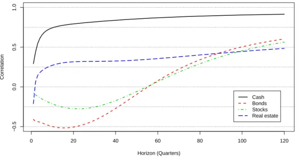
To investigate the inflation-hedging properties of the asset classes, we first analyze the correlations between the assets and inflation implied by the VAR model, depending on the investment horizon as in Hoevenaars, Molenaar, Schotman, and Steenkamp (2008), Amenc, Martellini, Milhau, and Ziemann (2009) and Briere and Signori (2012). Figure 2.1 shows the correlations between nominal asset returns and inflation, depending on the investment horizon. The correlations between cash and inflation are always positive and increase over the investment horizon, reaching a coefficient of around 90% at a 30-year horizon. Cash exhibits by far the highest correlations, with real estate exhibiting the second highest (and most positive) correlations up to horizons of 22 years, except for very short horizons. According to the correlations, bonds and stocks exhibit poor inflation-protecting qualities for short and medium horizons, but the hedging abilities of these two assets improve with the investment horizon and are better than those of real estate in the long run.

It is important to note that the correlation statistics only measure the linear relationship between the asset returns and the inflation rate. Thus, any conclusions about inflation-hedging abilities can be misleading. An asset class could move in conjunction with the inflation rate and would have a high positive correlation with inflation. However, if the inflation rate is always higher than the asset return, that asset would be a bad inflation hedge despite its positive correlation with inflation.

To further explore the potential of cash, bonds, stocks and real estate to protect against inflation, we measure the risk of the assets to fall below the inflation rate.

In particular, we consider LPMs of orders 0 (shortfall probability), 1 (expected shortfall) and 2 (semivariance) for various investment horizons. To calculate these horizon-dependent risk measures, we bootstrap nominal returns of lengthk, ranging

(28)

Figure 2.1: Correlations between Asset Returns and Inflation

Horizon (Quarters)

Correlation

0 20 40 60 80 100 120

−0.50.00.51.0

Cash Bonds Stocks Real estate

Notes: This figure shows correlations between the nominal asset returns and inflation depending on the investment horizon.

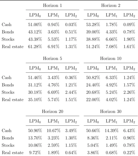
from four quarters (one year) to 120 quarters (30 years). Note that real estate, contrary to cash, bonds and stocks, is characterized by high transaction costs, which reduces the returns. To account for this fact, we adjust the generated returns by the transaction costs, except for cash.¹³ Following Rehring (2012), we assume round-trip transaction costs for bonds and stocks of 0.1% and 1%, respectively. These costs include bid-ask spreads and brokerage commissions. The round-trip transaction costs for direct real estate are generally assumed to be around 7% and they consist of transfer taxes and professional fees. Table 2.3 gives the LPMs with the inflation rate as the target for the assets analyzed.

We find that the inflation-hedging characteristics of the assets are different than those obtained from the correlation analysis. Although cash is the best inflation hedge for investment horizons up to five years, as indicated by the lowest expected shortfall and semivariance, the LPMs of orders 1 and 2 of this asset class increase with the investment horizon. Moreover, if we follow Briere and Signori (2012), and

13Transaction costs for cash are typically very low. Luttmer (1996) reports bid-ask spreads of 3 basis points for T-bills, which we disregard here.

(29)

Table 2.3: Lower Partial Moments of the Asset Returns

Horizon 1 Horizon 2

LPM₀ LPM₁ LPM₂ LPM₀ LPM₁ LPM₂

Cash 51.00% 0.94% 0.03% 53.28% 1.78% 0.09%

Bonds 43.12% 3.63% 0.51% 39.00% 4.33% 0.78%

Stocks 43.38% 5.53% 1.17% 38.88% 6.66% 1.90%

Real estate 61.28% 6.91% 1.31% 51.24% 7.08% 1.61%

Horizon 5 Horizon 10

LPM₀ LPM₁ LPM₂ LPM₀ LPM₁ LPM₂

Cash 51.46% 3.43% 0.36% 50.82% 6.33% 1.24%

Bonds 31.12% 4.76% 1.21% 24.40% 4.92% 1.57%

Stocks 30.18% 6.69% 2.44% 20.68% 5.24% 2.26%

Real estate 35.10% 5.74% 1.51% 22.00% 4.02% 1.24%

Horizon 20 Horizon 30

LPM₀ LPM₁ LPM₂ LPM₀ LPM₁ LPM₂ Cash 50.90% 10.67% 3.49% 50.66% 14.39% 6.43%

Bonds 13.70% 3.23% 1.30% 8.36% 2.11% 0.96%

Stocks 10.06% 2.59% 1.15% 5.04% 1.49% 0.78%

Real estate 9.72% 1.89% 0.64% 3.86% 0.68% 0.22%

Notes: This table reports lower partial moments of order zero, one and two with the inflation rate as target for the assets cash, bonds, stocks and real estate and for various investment horizons (1, 2, 5, 10, 20 and 30 years).

(30)

consider only shortfall probabilities while disregarding the amount of shortfall to assess inflation-protecting properties, we also obtain different results. The shortfall probabilities of cash are continuously over 50% and are higher than those of all other asset classes for investment horizons longer than one year. According to first and second-order LPMs, bonds, stocks and real estate exhibit weaker inflation- protecting properties in the short run. However, increasing the investment horizon results in a different picture. For investment horizons of 10 years or longer, real estate provides the best downside inflation protection compared to the other assets analyzed, as indicated by the LPMs of all orders for 10 to 30-year horizons (except for the shortfall probability at horizon of 10 years). We find that bonds perform better than stocks with respect to the expected shortfall and the semivariance up to a 10-year investment horizon. For longer horizons, equities are a better inflation hedge than bonds. Cash exhibits the poorest inflation-protecting properties in the long run. While the expected shortfall and semivariance of the other asset classes do not exceed 2.11% and 0.96%, respectively, the expected amount of cash to fall below the inflation rate is 14.39% and the semivariance is 6.43%. In addition, the shortfall probabilities confirm the weak inflation-hedging performance of cash compared to bonds, stocks and real estate in the long run.

If we compare the results of the correlation analysis with those of the LPM analysis, we obtain different results for the inflation-hedging performance of assets. We thus conclude that high correlations do not necessarily imply low LPMs. The ten- dency for the inflation-hedging abilities of bonds, stocks and real estate to improve along with the investment horizon is indicated by both the correlations and the LPMs. But, the results for cash differ significantly. Furthermore, according to the correlations, real estate exhibits the poorest inflation-hedging qualities in the long run, but the best qualities with respect to the downside risk measures.

2.3.4 Inflation-Protecting Asset Allocation

We now explore the optimal asset allocations for investors who aim to protect their portfolios against inflation. We investigate the optimal portfolios for investors with a real return target of 0% as well as for more ambitious investors with real return

(31)

targets ranging from 1% to 3%.¹⁴ Our investigations also consider various investment horizons.

As we did for the LPM analysis in the previous section, we again use bootstrapped and transaction cost-adjusted (real) returns of length k (with k varying from four quarters to 120 quarters) for 10,000 paths to construct minimum semivariance portfolios. We begin by examining optimal portfolios for an investor who simply desires to protect her portfolio against inflation, which implies a target real return of 0%.

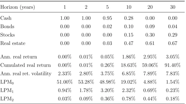
Table 2.4 shows minimum semivariance portfolios with a real return target of 0% at different investment horizons.

Table 2.4: Minimum Semivariance Portfolios with Real Return Target of 0%

Horizon (years) 1 2 5 10 20 30

Cash 1.00 1.00 0.95 0.28 0.00 0.00

Bonds 0.00 0.00 0.02 0.10 0.09 0.04

Stocks 0.00 0.00 0.00 0.15 0.30 0.29

Real estate 0.00 0.00 0.03 0.47 0.61 0.67

Ann. real return 0.00% 0.01% 0.05% 1.86% 2.95% 3.05%

Cumulated real return 0.00% 0.01% 0.26% 18.63% 59.06% 91.40%

Ann. real ret. volatility 2.33% 2.80% 3.75% 6.85% 7.89% 7.83%

LPM₀ 51.00% 53.28% 48.98% 19.02% 4.88% 1.54%

LPM₁ 0.94% 1.78% 3.20% 2.32% 0.69% 0.23%

LPM2 0.03% 0.09% 0.36% 0.78% 0.44% 0.18%

Notes: This table reports minimum semivariance portfolios with a real return target of 0% for various investment horizons (1, 2, 5, 10, 20 and 30 years) and corresponding descriptive statistics below. ”Ann./ret.” are the abbreviations for ”Annualized/return”.

Note that the shortfall probability and the expected shortfall are much lower for long-horizon investments over 20 or 30 years than for one or two-year investments. Moreover, the annualized real return and the annualized real return volatility increase with the investment horizon (except for the 30-year horizon where the volatility slightly decreases).

14Note that our results are not affected by considering real returns with a real return target of 0. Thus, instead of nominal returns with the inflation rate as the target, we switch to real terms from hereon in order to simplify the presentation of the results.

(32)

At the one and two-year horizons, the minimum semivariance portfolio is en- tirely invested in cash. This result is not surprising, however, since we have found that cash would be the best inflation-hedging asset in the short run. Both portfolios perceive real capital, as indicated by slightly positive annualized real returns.

The probability of falling below the inflation rate is relatively high with values of 51% and 53% for the one and two-year horizon minimum semivariance portfolios, respectively. These portfolios have an expected shortfall of 0.94% and 1.78% and semivariances close to 0%. Because cash is the only asset included in the portfolios, there are no diversification benefits and the risk measures are equal to the results in Table 2.3. For a five-year investment horizon, the weight of cash remains quite high at 95%, with only 2% and 3% invested in bonds and real estate. If we consider longer investment periods, we see that the weights change substantially. For a 10-year horizon, the optimal inflation-protecting asset allocation is 28% cash, 10%

bonds, 15% stocks and 47% real estate. This portfolio has an annualized real return of 1.86% and an annualized real return volatility of 6.85%. We also obtain diversification benefits from allocating various assets. The LPMs of all orders are lower than those of the single assets at a 10-year investment horizon. Note that, in the previous section, stocks were found to exhibit good inflation-hedging qualities as the investment horizon increased, which were taken into account for the long horizon portfolios. While cash plays no role in long horizon inflation-hedging portfolios, the proportion assigned to stocks doubles, with weights of 30% and 29%, respectively, in the optimal portfolio with a horizon of 20 and 30 years. Real estate was found to be the best inflation-hedging asset for investment horizons of 10 years or longer, so more than 50% of investor’s capital should be invested in this asset class in the long run. Moreover, the allocations to bonds over the long term are small compared to stocks and real estate. For the optimal portfolio with a 30-year investment horizon, the weight of bonds is only 4%.

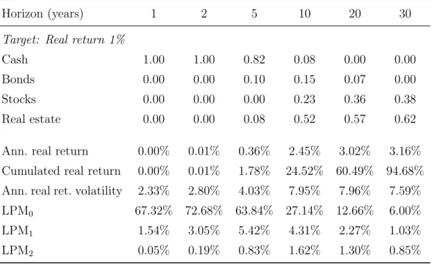
Assuming next an investor with a more performance-oriented goal, we also examine optimal semivariance portfolios with higher real return targets. Table 2.5 shows minimum semivariance portfolios with real return targets of 1%, 2% and 3%

at various investment horizons.

(33)

Intuitively, we would expect that imposing a higher target return would lead to portfolios with more risk. Although the composition of the short-run portfolios and, consequently, the LPMs do not change with the different target rates, the risk measures of the medium and long-term portfolios increase substantially. For example, at a five-year investment horizon, the minimum semivariance portfolio with a target real return of 0% falls below the inflation rate with a probability of 48.98%.

Increasing the target real return to 1%, 2% and 3% yields shortfall probabilities of 63.84%, 69.30% and 71.14%, respectively. The other risk measures, the expected shortfall and the semivariance, also rise with an increasing target return. The higher portfolio risk is caused by shifting more weight to assets that are more volatile than cash. Considering a five-year horizon, investors who require an additional premium decrease their allocations to cash (down to 38% for the 3% target) and invest more in bonds, stocks and real estate compared to investors who seek to preserve their capital and invest more than 90 % in cash. Apart from cash, substantial amounts of bonds and real estate are allocated at five-year investment horizons. As horizon and target rates increase, the weights of bonds (and to some extent, real estate) shift to stocks, making equities an interesting asset class for the long run. However, real

Table 2.5: Minimum Semivariance Portfolios with Positive Real Return Targets

Horizon (years) 1 2 5 10 20 30

Target: Real return 1%

Cash 1.00 1.00 0.82 0.08 0.00 0.00

Bonds 0.00 0.00 0.10 0.15 0.07 0.00

Stocks 0.00 0.00 0.00 0.23 0.36 0.38

Real estate 0.00 0.00 0.08 0.52 0.57 0.62

Ann. real return 0.00% 0.01% 0.36% 2.45% 3.02% 3.16%

LPM₀ 67.32% 72.68% 63.84% 27.14% 12.66% 6.00%

LPM₁ 1.54% 3.05% 5.42% 4.31% 2.27% 1.03%

LPM₂ 0.05% 0.19% 0.83% 1.62% 1.30% 0.85%

Continued

(34)

Continued

Cash 1.00 1.00 0.60 0.00 0.00 0.00

Bonds 0.00 0.00 0.20 0.17 0.00 0.00

Stocks 0.00 0.00 0.06 0.30 0.45 0.41

Real estate 0.00 0.00 0.14 0.53 0.55 0.59

Ann. real return 0.00% 0.01% 0.89% 2.72% 3.12% 3.21%

LPM₀ 80.24% 87.04% 69.30% 39.40% 27.36% 19.08%

LPM1 2.28% 4.65% 7.66% 7.35% 6.10% 4.41%

LPM₂ 0.09% 0.34% 1.57% 2.94% 3.32% 2.98%

Cash 1.00 1.00 0.38 0.00 0.00 0.00

Bonds 0.00 0.00 0.31 0.14 0.00 0.00

Stocks 0.00 0.00 0.11 0.35 0.49 0.48

Real estate 0.00 0.00 0.20 0.51 0.51 0.52

Ann. real return 0.00% 0.01% 1.45% 2.78% 3.16% 3.25%

LPM₀ 90.10% 94.70% 71.14% 53.72% 45.94% 41.84%

LPM₁ 3.14% 6.47% 10.11% 11.91% 13.36% 13.34%

LPM₂ 0.14% 0.56% 2.55% 4.99% 7.44% 8.75%

Notes: This table reports minimum semivariance portfolios with real return targets of 1%, 2% and 3% for various investment horizons (1, 2, 5, 10, 20 and 30 years) and corresponding descriptive statistics below. ”Ann./ret.” are the abbreviations for ”An- nualized/return”.

(35)

estate appears to be the most attractive asset for investors willing to hedge inflation and also for performance-oriented investors with a 10-year or longer investment horizon.

2.4 Conclusion

In this paper we investigated the inflation-protecting abilities of cash, bonds, stocks and direct real estate and optimal asset allocations between these assets for investors seeking to preserve real capital or to achieve a return exceeding the inflation rate.

We captured the dynamics of asset returns and the inflation rate by a VAR model to analyze horizon-dependent correlations between assets and inflation. Moreover, using the VAR framework, we generated multi-period asset returns to investigate lower partial moment risk measures of the assets over various investment horizons.

These bootstrap-based returns were also used to determine horizon-dependent optimal inflation-hedging asset allocations within a downside risk framework.

We find that the standard approach of considering only correlations to analyze the inflation-hedging properties of assets can be misleading. Comparing correlation results with those of an LPM analysis shows very different findings. According to the correlations, cash is the best inflation-hedging asset over all horizons and real estate exhibits the poorest inflation-protecting ability in the long run. In the downside risk analysis, however, we find that cash hedges again inflation best only in the short run, while real estate actually has the best inflation protection qualities for medium and long horizons. We also find that bonds and stocks improve their inflation-hedging abilities along with the investment horizon. These changes in the inflation-hedging properties of cash, stocks, bonds and real estate over the investment horizon also affect the optimal inflation-protecting asset allocations. While cash is the only relevant asset for short-term optimal inflation-hedging portfolios, real estate plays the most important role in medium and long-term portfolios. In our asset allocation analysis, we consider not only an investor who desires to preserve capital, but also an investor with a more performance-oriented target. Increasing the target return, i.e. examining an investor who requires a premium in excess of the inflation rate, we find that larger weights are assigned to more risky assets compared to cash. On

(36)

a medium and long-term basis, the highest amount of the investor’s capital should be invested in real estate. Equities also become highly attractive for investors who require a positive real return in the long run.

Our study has only investigated the role of the most widely used assets: cash, bonds, stocks and real estate, with respect to inflation-hedging but can be extended to other asset classes. It would seem sensible to include inflation-linked bonds in the analysis of inflation protection. However, the length of available time series is too short for an econometric analysis without any concerns. The same argument also applies to the inclusion of alternative investment classes such as infrastructure, which is currently of great interest to many investors.

(37)

Modeling Asset Price Dynamics under a Multivariate

Cointegration Framework

This paper is the result of a joint project with Benedikt Fleischmann.

Abstract

We show that allowing for cointegration within a vector autoregressive (VAR) framework yields important implications for modeling the asset price dynamics of T-bills, stocks and bonds over all investment horizons. While the stationary VAR approach ignores common stochastic trends of the included variables, the vector error correction (VEC) model captures these common long-run relations and their predictable restorations. We find interesting differences in the term structure of risk of the VEC compared to the traditional VAR. There is a strong positive link between risk premia and real interest rates in the short term and a much more negative and longer-lasting impact of inflation on excess stock and bond returns. Incorporating cointegration significantly shifts downward nominal stock and bond volatilities and incorporates inflation as the driving component of nominal interest rates, which results in a flat risk structure of real interest rates. For an extreme risk-averse investor, the optimal real (nominal) return portfolio is tilted much more towards T-bills (bonds).

(38)

3.1 Introduction

In recent empirical finance research, the stationary vector autoregressive (VAR) model is a popular framework for modeling long-run asset price dynamics.¹ In the multi-horizon context, the VAR has some convenient advantages compared to the simple regression model. First, this approach makes it possible to study the inter- actions between asset prices and economic state variables as well as the pulling and pushing forces going through certain economic channels. Second, long-term effects can easily be explored by iteratively calculating multi-period forecasts. Hence, the model estimated by short-run dynamics is able to capture long-horizon behavior.

Third, while simple long-horizon regressions are often criticized due to their sta- tistical properties (biased t-statistics), the VAR shows no econometric issues with respect to long-run forecasts. Therefore, the VAR setup is often used to account for predictability and to capture time-varying investment opportunities of several assets such as cash, stocks and bonds simultaneously.

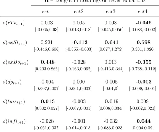
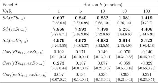
However, we argue that the stationary VAR approach ignores important additional information as it does not consider the presence of common long-run relations between the assets and the state variables. Deviations in the long-term comovement of the variables cause predictable backward movements. These cointegration effects can be incorporated into an extension of the VAR model, the vector error correction (VEC) model. Allowing for cointegration yields important implications for the in- terdependencies among the variables at all horizons. We observe a significant change in the horizon-dependent risk structure of the asset returns and ultimately that the optimal portfolio rules are substantially different from the stationary VAR model.

The framework of cointegration and error correction has been used in several other studies and goes back to Granger (1981) and Engle and Granger (1987). Campbell and Shiller (1987) test cointegration between dividends and stock prices as well as long-term bond yields and short-term interest rates. They detect the dividend-

1Some examples of authors using the VAR methodology to account for predictability and horizon effects of asset returns include: Campbell and Shiller (1988a,b); Campbell (1991); Campbell and Ammer (1993); Kandel and Stambaugh (1996); Barberies (2000); Campbell, Chan, and Viceira (2003); Campbell and Viceira (2005); Hoevenaars, Molenaar, Schotman, and Steenkamp (2008);

Jurek and Viceira (2011).

(39)

price ratio and term spread to be stationary and restoring to their means, while the deviations can be quite persistent. Nasseh and Strauss (2000) find significant cointegration relations between stock prices and macroeconomic variables in six Eu- ropean countries. Other academic researchers emphasize a long-run relationship between consumption and dividends containing important information about the variances and means of cash flows and, by implication, their returns (Bansal, Gal- lant, and Tauchen, 2007; Hansen, Heaton, and Li, 2008; Bansal, Dittmar, and Kiku, 2009; Bansal and Kiku, 2011). Bansal, Dittmar, and Kiku (2009) and Bansal and Kiku (2011) incorporate this error correction information into the VAR framework (EC-VAR) and conclude that the dynamics are better captured compared to the traditional VAR. As a consequence, the risk premium and the term structure of risk can be distorted by neglecting cointegration. Furthermore, Lettau and Ludvigson (2001) and Lettau and Ludvigson (2005) motivate cointegration between consumption, labor income and financial wealth (cay). They find that cay outperforms popular stock return predictors such as the dividend-price ratio for short as well as long horizons. Hence, cointegration can handle the deviation of asset prices from the fundamental equilibrium in boom and bust cycles and predict their restorations.

Additionally, more recent studies use a VEC appproach to model price and return dynamics of financial securities (e.g. Zhong, Darrat, and Anderson, 2003; Blanco, Brennan, and Marsh, 2005; Durre and Giot, 2007; Barnhart and Giannetti, 2009).

These findings and studies motivate an extension of the stationary VAR model by cointegration and the integration of common long-run relationships into a long-run asset pricing analysis. If the time series used in the traditional VAR are differenced in order to obtain stationarity, their stochastic trends are eliminated. Although this procedure is quite common, it is disadvantageous for cointegrated variables and always leads to a distortion of the relationships between the variables analyzed.

However, the magnitude and the direction of this bias remain unclear and depend on the investment horizon.

Therefore, we contribute to the literature by comparing the stationary VAR and the VEC model with respect to their modeled short- and long-run behavior, where both models include the same set of investable assets (T-bills, stocks and bonds) and common state variables that have been shown to predict returns (dividend-