Asset Allocation under the Influence of Long-Run Relations

zu Immobilienökonomie und Immobilienrecht

Herausgeber:

IRE

I

Prof. Dr. Sven Bienert

Prof. Dr. Stephan Bone-Winkel Prof. Dr. Kristof Dascher Prof. Dr. Dr. Herbert Grziwotz Prof. Dr. Tobias Just

Prof. Dr. Kurt Klein

Prof. Dr. Jürgen Kühling, LL.M.

Prof. Gabriel Lee, Ph. D.

Prof. Dr. Gerit Mannsen

Prof. Dr. Dr. h.c. Joachim Möller Prof. Dr. Wolfgang Schäfers

Prof. Dr. Karl-Werner Schulte HonRICS Prof. Dr. Steffen Sebastian

Prof. Dr. Wolfgang Servatius Prof. Dr. Frank Stellmann Prof. Dr. Martin Wentz

Benedikt Fleischmann

Asset Allocation under the

Influence of

Long-Run

Relations

Benedikt Fleischmann

Asset Allocation under the Influence of Long-Run Relations

Fleischmann, Benedikt

Asset Allocation under the Influence of Long-Run Relations Benedikt Fleischmann

Regensburg: Universitätsbibliothek Regensburg 2014

(Schriften zu Immobilienökonomie und Immobilienrecht; Bd. 71) Zugl.: Regensburg, Univ. Regensburg, Diss., 2013

ISBN: beantragt

ISBN: beantragt

© IRE|BS International Real Estate Business School, Universität Regensburg Verlag: Universitätsbibliothek Regensburg, Regensburg 2014

Zugleich: Dissertation zur Erlangung des Grades eines Doktors der Wirtschaftswissenschaften, eingereicht an der Fakultät für Wirtschaftswissenschaften der Universität Regensburg

Tag der mündlichen Prüfung: 24. Juli 2013 Berichterstatter: Prof. Dr. Steffen Sebastian

Prof. Dr. Rolf Tschernig

1 Research Objectives, Methods and Scientific Contributions 1 2 Inflation-Hedging, Asset Allocation and the Investment Horizon 6

2.1 Introduction . . . 7

2.2 Literature Review . . . 8

2.3 VAR Model and Data . . . 11

2.3.1 VAR Specification . . . 11

2.3.2 Data . . . 13

2.3.3 VAR Estimates . . . 14

2.4 Horizon Effects in Risk and Return for Nominal and Real Returns . . . 18

2.4.1 The Term Structure of Risk . . . 18

2.4.2 Inflation-Hedging . . . 22

2.4.3 The Term Structure of Expected Returns . . . 25

2.5 Horizon-Dependent Portfolio Optimizations . . . 27

2.5.1 Mean-Variance Optimization . . . 27

2.5.2 Results . . . 28

2.6 Conclusion . . . 31

2.A Appendix . . . 32

2.A.1 Data . . . 32

2.A.2 Calculation of the Desmoothed Real Estate Returns . . . 32

2.A.3 Robustness Regarding Different Unsmoothing Parameters . . . 33

2.A.4 Misspecification Tests . . . 35

3 Modeling Asset Price Dynamics under a Multivariate Cointegra-

tion Framework 37

3.1 Introduction . . . 38

3.2 Methodology . . . 41

3.2.1 VAR Specification . . . 41

3.2.2 VEC Specification . . . 42

3.2.3 Horizon Dependent Variance-Covariance . . . 43

3.2.4 Portfolio Choice Problem . . . 45

3.3 Empirical Analysis . . . 47

3.3.1 Data and Time Series Properties . . . 47

3.3.2 Estimation Results . . . 51

3.3.3 Long Horizon Effects . . . 59

3.3.4 Asset Allocation Decisions . . . 67

3.4 Conclusion . . . 72

3.A Appendix . . . 74

3.A.1 Bootstrap Method . . . 74

3.A.2 Model Selection . . . 75

4 Do Stock Prices and Cash Flows Drift Apart? The Influence of Macroeconomic Proxies 76 4.1 Introduction . . . 77

4.2 Methodology . . . 79

4.2.1 The Econometric Model . . . 80

4.2.2 Hypotheses Testing . . . 81

4.2.3 Long-Run Analyses . . . 83

4.2.4 Returns . . . 84

4.3 Empirical Analysis . . . 85

4.3.1 Data and Time Series Properties . . . 85

4.3.2 Cointegration Rank Analysis . . . 90

4.3.3 Restriction Tests . . . 93

4.3.4 Testing the Financial Ratios . . . 96

4.3.5 Level Effects . . . 98

4.3.6 Horizon-Dependent Analysis . . . 100

4.4 Conclusion . . . 104

4.A Appendix . . . 106

4.A.1 Model Selection . . . 106

4.A.2 Univariate Stationarity of the Financial Ratios . . . 107

4.A.3 Stability of the Long-Run Matrices across the Models . . . 108

4.A.4 Bootstrap Method . . . 110

Bibliography 111

2.1 Conditional Standard Deviations of the Assets . . . 20

2.2 Conditional Standard Deviation of the Inflation . . . 21

2.3 Conditional Correlations of Asset Returns and Inflation . . . 24

4.1 Level Variables . . . 88

4.2 Differenced Variables . . . 89

4.3 Impulse Response Functions . . . 101

4.4 Impulse Response Functions of Returns . . . 103

2.1 Summary Statistics . . . 15

2.2 VAR Estimation Results . . . 16

2.3 Term Structure of Expected Returns . . . 26

2.4 Portfolio Calculations . . . 29

2.5 Data Information . . . 32

2.6 Results Regarding Different Unsmoothing Parameters . . . 34

2.7 VAR Order Selection . . . 35

2.8 Residual Tests . . . 36

3.1 Abbreviationsg . . . 48

3.2 Descriptive Statistics . . . 49

3.3 Simultaneous and Lagged Correlations . . . 50

3.4 Unit Root and Cointegration Rank Test . . . 51

3.5 VAR Parameter Estimatesg . . . 52

3.6 VEC Parameter Estimatesg . . . 55

3.7 Term Structure of Risk and Correlationsg. . . 60

3.8 Variance Decomposition for Treasury Bills . . . 62

3.9 Variance Decomposition for Stock Returns . . . 63

3.10 Variance Decomposition for Bond Returns . . . 66

3.11 Global Minimum Variance Portfoliosg . . . 69

3.12 Optimal Portfolio Holdings for γ = 20 . . . 70

3.13 Lag Length Selection . . . 75

4.1 Univariate Stationarity . . . 86

4.2 Descriptive Statistics . . . 87

4.3 Cointegration Rank . . . 92

4.4 β Restriction Tests . . . 94

4.5 α Restriction Tests . . . 95

4.6 Financial Ratio Stationarity Tests . . . 97

4.7 Πr Matrix of Model M6 and r= 4 . . . 99

4.8 Lag Length Selection and Cointegration Rank Stability . . . 106

4.9 Univariate Stationarity of Financial Ratios . . . 107

4.10 Stability Analysis of the Long-Run Matrices . . . 109

Research Objectives, Methods and Scientific Contributions

Inflation-Hedging, Asset Allocation and the Invest- ment Horizon

Most of the empirical studies falsify the inflation-hedging hypothesis of stocks and real estate, but they typically establish their research methods on quarterly to annual returns and, therefore, contrast with the fact that most investors have much longer investment horizons. Additionally, the perverse inflation-hedging characteristics of stocks and real estate run contrary to the general economic theory that these assets should be a good hedge against inflation. The residual claims of the investors are the cash flows and retained earnings, and these are derived from real assets.

In our paper ’Inflation-Hedging, Asset Allocation and the Investment Horizon’, my coauthors, Christian Rehring and Steffen Sebastian, and I link the inflation- hedging analysis to the mixed asset allocation analysis focusing on the role of the investment horizon for a buy-and-hold investor. Using a vector auto-regression (VAR) for the UK market, we estimate correlations of nominal returns with infla- tion to analyze how the inflation-hedging abilities of cash, bonds, stocks and direct commercial real estate change with the investment horizon. In doing so, we find that the inflation-hedging characteristics of all assets improve with the investment horizon. Cash is clearly the best inflation hedge at short and medium horizons. For

long horizons, direct real estate hedges unexpected inflation as well as cash. These results have implications for the difference between the term structures of annual- ized volatilities of real versus nominal returns, and ultimately for portfolio choice.

While cash is very attractive for short-horizon investors, it is much less attractive at medium and long horizons. The allocation to real estate is strongly increasing with the investment horizon; due to the favorable inflation-hedging abilities, real estate is more attractive for an investor concerned about inflation. Bonds are less attractive for an investor taking into account inflation. The differences in the opti- mal asset weights (based on real versus nominal returns) can be interpreted as the mistake that an investor subject to inflation illusion makes respectively providing information about the inflation-hedging qualities of the single assets in a portfolio context. The differences between the real and nominal asset allocation results can be substantial.

Modeling Asset Price Dynamics under a Multivari- ate Cointegration Framework

The stationary vector autoregressive (VAR) model is a popular framework for mod- eling long-run asset price dynamics in the empirical finance research. This approach allows to study the interactions between asset prices and economic state variables as well as the pulling and pushing forces going through certain economic channels.

However, the stationary VAR approach ignores important additional information as it does not consider the presence of common long-run relations between the assets and state variables. Under cointegration, deviations of the long-term comovement of the variables cause predictable backward movements.

Therefore, in our paper ’Modeling Asset Price Dynamics under a Multivariate Cointegration Framework’, my coauthor, Tim Koniarski, and I contribute to the literature by comparing the stationary VAR and the VEC approach with respect to their modeled short and long-run behavior, where both models include the same set of investable assets (T-bills, stocks and bonds) and common state variables that have been shown to predict returns (dividend-price ratio, term spread and inflation).

Starting from a VAR representation, we find strong evidence for common stochastic trends between the levels of the six variables. The cointegration rank test indicates four cointegration relations among the level variables. While the standard VAR model captures only the long-run dynamics of stationary data, the VEC model takes into account information about the four cointegration relations and is able to distinguish between short and long-run effects. The estimation results show a more than two times higher adjusted R² for the risk premia of stocks and bonds for the VEC. These increases already show the importance of incorporating common long-run effects in the analysis of asset price dynamics. This motivates a further comparison of the long-run dynamics implied by the VAR and VEC, depending on the time horizon, by investigating the variance decompositions of real and nominal asset returns. Therefore, we examine the various risk components of the returns, their interactions and sources. We find substantial differences between the two models with respect to the term structure of risk. The VEC shows a much higher correlation between the risk premia and real interest rate in short and medium horizons as well as a much more negative correlation between the risk premia and inflation in the long run. As a further finding, the volatilities of nominal returns are significantly lower under cointegration over all horizons. Turning to real terms, we find the same evidence for stock returns and, moreover, the term structure of T-bills appears roughly flat compared to the mean-averting structure of the stationary VAR.

The latter result indicates a strong common stochastic trend between nominal T-bills and inflation. Finally, these differences in the risk structure influence the optimal portfolio choice. Under cointegration the global minimum variance portfolio of real (nominal) returns is much more tilted towards T-bills (bonds). In the VEC, a less risk-averse investor has a much higher equity exposure as the investment horizon lengthens and even leverages the position in the very long run. This behavior is borne by a decreasing bond position compared to the VAR model.

Do Stock Prices and Cash Flows Drift Apart? The Influence of Macroeconomic Proxies

Several studies in the predictability literature use variables such as the dividend- price ratio and earnings-price ratio to forecast stock returns. According to theory, stock prices are the discounted future cash flows and, therefore, should move around their fundamentals (dividends and earnings) in the long run. Hence, it is generally assumed that prices and cash flows are cointegrated one-for-one or, alternatively, that the dividend-price ratio and earnings-price ratio are stationary variables, since otherwise the conventional t-statistics lead to wrong conclusions about the evidence of return predictability.

In our paper ’Do Stock Prices and Cash Flows Drift Apart? The Influence of Macroeconomic Proxies’, my coauthor, Tim Koniarski, and I extend the loglinear Campbell and Shiller (1988a) model to investigate the influences of macroeconomic variables (inflation, short-term interest rates, government and corporate bond yields) on stock prices and cash flows (dividends and earnings) and, consequently, the im- plied impacts on total stock returns. The versatile model setup enables us to test the validity of the stationarity of the dividend-price ratio in a multivariate framework.

Moreover, in the same way we also examine the stationarity of further financial ra- tios such as dividend-earnings, earnings-price, real short-interest rates, term spread and credit spread, which are additionally used in the predictability literature. Our tests show that dividend-earnings and the term spread most likely are stationary or, alternatively, that the underlying variables have the same stochastic trends, whereas the null hypothesis of stationarity is rejected for the remaining ratios. Additionally, we find inflation to have a strong impact on the equity market. While other papers often consider returns, prices and dividends in real terms to avoid inflation effects and assume that inflation influences equity market variables identically, we show a negative linkage between nominal prices and inflation and nominal cash flows to be positively associated to inflation in the long run. Thus, nominal total stock re- turns are reduced by inflation shocks in the short term, but recover for long time horizons. This result connects the contrary findings of Fama and Schwert (1977) and Boudoukh and Richardson (1993), and enforces the findings of my first paper

’Inflation-Hedging, Asset Allocation and the Investment Horizon’. Moreover, we find that interest rates play a similar role for all equity market variables. Although prices, dividends and earnings are reduced by rising interest rates, the magnitude is much more pronounced for cash flows than for stock prices. Finally, while for corporate bond yields we find large positive effects on the equity market, the influences of the government bond yields are negative.

Inflation-Hedging, Asset

Allocation and the Investment Horizon

This paper is the result of a joint project withChristian Rehring and Steffen Sebas- tian.

Abstract

Focusing on the role of the investment horizon, we analyze the inflation-hedging abilities of stock, bond, cash and direct real estate investments. Based on vector autoregression for the UK market, we find that the inflation-hedging characteristics of all assets improve with the investment horizon. For long horizons, direct real estate seems to hedge unexpected inflation as well as cash. This has important implications for the risk structure of real versus nominal returns of the assets de- pending on the investment horizon, and ultimately for portfolio choice. Switching from nominal to real returns, real estate becomes more attractive with very high long-term allocations. In contrast, bonds are less attractive for an investor taking inflation into account.

2.1 Introduction

The monetary base has grown considerably in many economies as a reaction to the recent financial crisis. As a result, the fear of inflation has regained attention. Even modest inflation rates can have a significant effect on the real value of assets. While persistency makes the level of inflation well predictable in the short run, this effect turns upside down in the long term, making inflation a key variable for long-term portfolio decisions. Accordingly, assets that hedge inflation are desirable for private investors who are concerned about the purchasing power of their investments as well as for institutional investors whose liabilities are linked to inflation (such as pension funds). Despite the important role of inflation for decision-making, people often think in nominal rather than real terms, a phenomenon referred to as “money illusion” (for a review see Akerlof and Shiller, 2009, Chapter 4).

Most of the empirical studies falsify the inflation-hedging hypothesis of stocks and real estate, but they typically use quarterly or annual returns. The perverse inflation-hedging characteristics run contrary to the general economic theory that assets should be a good hedge against inflation due to the fact that they are claims to cash-flows derived from real assets. However, studies based on quarterly or annual returns contrast with the fact that most investors have longer investment horizons.

Due to return predictability, standard deviations (per period) and correlations of asset returns may change considerably with the investment horizon (Campbell and Viceira, 2005). Hence, the optimal asset allocation and inflation-hedging abilities depend on the investment horizon. The asset classes which are usually considered for a mixed asset allocation optimization are cash, bonds and stocks. But real estate is a further important asset class as it offers performance and diversification benefits. Moreover, practitioners often regard real estate investments to be a good inflation hedge. Direct real estate has high transaction costs, inducing substantial horizon effects in periodic expected returns (e.g. Collet, Lizieri, and Ward, 2003).

This is certainly a reason why direct real estate investments are typically long-term investments with an average holding period of about ten years (Collet, Lizieri, and Ward, 2003; Fisher and Young, 2000).

In this paper, we link the inflation-hedging analysis to the mixed asset allocation analysis focusing on the role of the investment horizon for a buy-and-hold investor.

Using a vector auto-regression (VAR) for the UK market, we estimate correlations of nominal returns with inflation to analyze how the inflation-hedging abilities of cash, bonds, stocks and direct commercial real estate change with the investment horizon.¹ In doing so, we find that the inflation-hedging characteristics of all assets improve with the investment horizon. These results have implications for the difference between the term structures of annualized volatilities of real versus nominal returns, and ultimately for portfolio choice. The differences in the optimal asset weights (based on real versus nominal returns) can be interpreted as the mistake that an investor subject to inflation illusion makes respectively providing information about the inflation-hedging qualities of the single assets in a portfolio context.

The remainder of the paper is organized as follows: In the next section, we review the related literature. A discussion of the VAR model, the data and the VAR results follow. Then, we analyze horizon effects in risk and return for nominal and real returns and discuss the inflation-hedging abilities of the assets. The asset allocation problem is examined in the next section, again distinguishing between nominal and real returns. Finally, the main findings are summarized.

2.2 Literature Review

Our paper contributes to two strands of literature: inflation-hedging and strategic asset allocation. Both fields are studied over different investment horizons, because long-term results can differ tremendously from short-term results.

The inflation-hedging literature starts with Bodie (1976), Jaffe and Mandelker (1976) and Fama and Schwert (1977). They find that nominal US stock returns are negatively related to realized inflation as well as to the two components of realized inflation, i.e. expected and unexpected inflation. Gultekin (1983) shows that the negative relation of nominal stock returns with inflation also holds for many

1Inflation-linked bonds with a maturity equal to the investment horizon are a particularly good inflation-hedge. Given the limited supply of these bonds, it is worthwhile to analyze the inflation- hedging abilities of common asset classes.

other countries. Bonds and bills provide a hedge against expected inflation, but not against unexpected inflation. Studies using the Fama and Schwert methodology and examining the direct commercial real estate market suggest at least a partial inflation hedge. US commercial real estate appears to offer a hedge against expected inflation, whereas the evidence with regard to unexpected inflation is not clear-cut (e.g. Brueggeman, Chen, and Thibodeau, 1984; Hartzell, Hekman, and Miles, 1987;

Gyourko and Linneman, 1988; Rubens, Bond, and Webb, 1989). Examining the UK market, Limmack and Ward (1988) find that commercial real estate returns are positively related to both expected and unexpected inflation. Depending on the proxy for expected inflation, however, commercial real estate does not appear to provide a hedge against both components.

The results of the above-cited studies are based on regressions with data that have a monthly to annual frequency. The disappointing short-term inflation-hedging abilities of most asset classes have motivated research in analyzing the long-term relation of asset returns with inflation. For both the US and the UK, Boudoukh and Richardson (1993) find positive relationships between five-year stock returns and realized as well as expected inflation, whereas annual returns show a negative or only weakly positive relationship. Hoesli, Lizieri, and MacGregor (2008), Luin- tel and Paudyal (2006) as well as Sch¨atz and Sebastian (2009) use error correction approaches to distinguish between short and long-term relationships between asset markets and macroeconomic variables. Hoesli, Lizieri, and MacGregor (2008) an- alyze the inflation-hedging abilities of stocks as well as direct and securitized real estate markets in the US and the UK. For all asset markets, they find a positive long- term relationship with expected inflation, while the long-term link to unexpected inflation is often negative. Luintel and Paudyal (2006) confirm the positive long- term relationship between UK stocks and inflation. Sch¨atz and Sebastian (2009) find a positive long-term link between commercial real estate markets and price indexes for both the UK and Germany. Confirming the findings of Hoesli, Lizieri, and MacGregor (2008), they observe that property markets in both countries are sluggish to adjust towards the long-term equilibrium existing with macroeconomic variables.

Several articles use a VAR approach to estimate horizon-dependent correlation statistics. As the predictability of the variables is taken into account, the inflation- hedging abilities of the assets are analyzed in terms of the correlation of unexpected asset returns with unexpected inflation. Campbell and Viceira (2005) find US stocks to hedge unexpected inflation in the very long-run (at the 50-year horizon). Hoeve- naars, Molenaar, Schotman, and Steenkamp (2008) calculate correlations between US asset returns and inflation shocks for horizons of up to 25 years. They find that cash is clearly the best inflation-hedge for investment horizons of one year and longer. Bonds are a perverse inflation hedge in the short run; the correlation turns positive after about 12 years to reach more than 0.5 after 25 years.

While the empirical evidence is not unambiguous, the general picture emerges is that the inflation-hedging abilities of assets improve with the investment horizon.

Nevertheless, there is no evidence about the long-term inflation-hedging abilities of direct real estate in a VAR framework.

Of course, the different inflation-hedging characteristics of the assets have port- folio implications. Intuitively, a highly positive correlation of nominal returns with inflation decreases the volatility of real returns on the asset. Hence, the better the inflation-hedging ability of the asset, the more attractive it is for an investor con- cerned about real returns. Schotman and Schweitzer (2000) show that when the investor is concerned about real returns, the demand for stocks in a portfolio with a nominal zero-bond (with a maturity that equals the investment horizon) depends on two terms. The first term reflects the demand due to the equity premium. The second term depends positively on the covariance of nominal stock returns with inflation and represents the inflation-hedging demand varying over the investment horizon.

Several articles calculate horizon-dependent risk statistics and optimal portfolio compositions based on real returns. Campbell and Viceira (2005) show that re- turn predictability induces major horizon effects in annualized standard deviations and correlations of real US stock, bond and cash returns. Stocks exhibit strong mean reversion, bonds exhibit slight mean reversion, whereas cash returns are mean averting. Thus, there are huge horizon effects in optimal portfolio compositions.

In addition to stocks, bonds and cash investments, Fugazza, Guidolin, and Nico-

dano (2007) consider European property shares, Fugazza, Guidolin, and Nicodano (2009) consider US REITs, whereas MacKinnon and Al Zaman (2009) consider US direct real estate.² While Fugazza, Guidolin, and Nicodano (2007) find property shares and REITs important in an investor’s portfolio, MacKinnon and Al Zaman (2009) weaken their result if an investor has access to the direct property market.

Hoevenaars, Molenaar, Schotman, and Steenkamp (2008) and Amenc, Martellini, Milhau, and Ziemann (2009) analyze the US market including securitized real es- tate as an asset class. Hoevenaars, Molenaar, Schotman, and Steenkamp (2008) emphasize that the dynamics of REIT returns are well captured by the dynamics of stock and bond returns, so that the opportunity to invest in securitized real estate does not add much value for the investor. Rehring (2012) studies the role of direct real estate in a mixed-asset portfolio over different investment horizons for the UK market. Considering transaction costs, he finds direct real estate to be important if the investor has a long horizon.

Analyzing the UK market, we follow the studies using a VAR approach. Given the huge importance of transaction costs for direct real estate investments, we account for the differing transaction costs of the asset classes. In contrast to previous studies, we compare risk, return and asset allocation results based on real versus nominal returns, which show the impact of the differing inflation-hedging abilities of the assets in a portfolio.

2.3 VAR Model and Data

2.3.1 VAR Specification

The basic framework follows Campbell and Viceira (2005), who introduce a model for long-term buy-and-hold investors. Let z_t+1 be a vector that includes log (con- tinuously compounded) asset returns and additional state variables that predict

2Hoevenaars, Molenaar, Schotman, and Steenkamp (2008) and Amenc, Martellini, and Ziemann (2009) extend the long-term asset allocation analysis based on VAR estimates to an asset-liability context, modeling the dynamics of liabilities of institutional investors.

returns. Assume that a VAR(1) model captures the dynamic relationships between asset returns and the additional state variables:

z_t+1 =Φ0 +Φ1z_t+ν_t+1. (2.1) In the specification of this study, the nominal return on cash (n0,t+1), and the excess returns on real estate, stocks, and long-term bonds (stacked in the (3×1) vector x_t+1 =n_t+1−n0,t+1ι, where ι is a vector of ones) are elements ofz_t+1. In addition, z_t+1 contains the realized inflation i_t+1, and three other state variables stacked in the (3×1) vectors_t+1 (the cap rate, the dividend yield and the yield spread). Thus,

z_t+1 =

















 n_0,t+1

x_t+1

it+1

s_t+1



















(2.2)

is of order (8×1). Φ0 is a (8×1) vector of constants andΦ1 is a (8×8) coefficient- matrix. The shocks are stacked in the (8×1) vector ν_t+1, and are assumed to be IID normal with zero means and covariance-matrix Σν, which is of order (8×8):

ν_t+1 ∼IIDN(0,Σν) with Σν =



















σ²₀ σ_0x σ_0i σ_0s σ_0x Σxx σ_ix Σsx

σ0i σ_ix σ²_i σ_is σ_0s Σ_sx σ_is Σss



















. (2.3)

The matrixΣconsists of the following block structure: the variance of nominal cash return shocks,σ₀², the covariance-matrix of excess return shocks,Σxx, the variance of inflation shocks,σ_i², and the covariance-matrix of the residuals of the state variables, Σss. The off-diagonal elements are the vector of covariances between shocks to the nominal return on cash and shocks to the excess returns on real estate, stocks and bonds,σ_0x, the covariance of shocks to the nominal cash return with inflation shocks, σ0i, the vector of covariances between shocks to the excess returns on real estate, stocks and bonds with inflation shocks,σ_ix, the vector of covariances between shocks to the nominal cash return and shocks to the state variables, σ_0s, the covariance matrix of shocks to the excess returns and shocks to the state variables, Σsx, and

the vector of covariances between inflation shocks and shocks to the state variables, σ_is.

2.3.2 Data

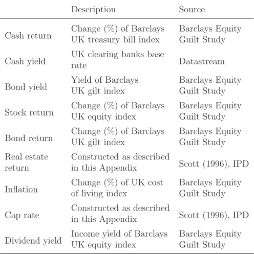
The results are based on an annual dataset from 1956 to 2010 (55 observations) for the UK market, the Appendix 2.A.1 provides more details on the data used.

As noted above, cash (T-bills), direct commercial real estate, stocks and long-term government bonds (gilts) are the assets available to the investor. The bond index represents a security with constant maturity of 20 years. The implicit strategy assumed here is to sell a bond at the end of each year and buy a new bond to keep the bond maturity constant, an assumption which is common for bond indexes. As in Campbell and Viceira (2005), the log of the dividend yield of the stock market and the log yield spread, i.e. the difference between the log yield of a long-term bond and the log yield of T-bills are incorporated as state variables that have been shown to predict asset returns. For direct real estate returns we include the (log of the) cap rate as a state variable that has been shown to predict direct real estate returns (Fu and Ng, 2001; Plazzi, Torous, and Valkanov, 2010; Rehring, 2012).

Appraisal-based capital and income real estate returns used to calculate the an- nual real estate total return and the cap rate series have been obtained from two sources. The returns from 1971 to 2010 are based on IPD’s long-term index. Returns from 1956 to 1970 are from Scott (1996).³ These returns are based on valuations of properties in portfolios of two large financial institutions covering more than 1,000 properties throughout this period (Scott and Judge, 2000).⁴ Key, Zarkesh, and Haq (1999) find that the Scott return series used here as well as the IPD 1971 to 1980 return series are fairly reliable in terms of coverage. Additionally the use of annual frequency avoid the stale appraisal problem. Real estate returns are unsmoothed using the approach of Barkham and Geltner (1994) because the original smoothed

3Note that due to the unsmoothing procedure for real estate returns, one additional observation is needed as shown in Appendix 2.A.2 .

4For comparison, the widely-used NCREIF Property Index (NPI) for the U.S. was based on only 233 properties at the index inception; see “Frequently asked questions about NCREIF and the NCREIF Property Index (NPI)” on the NCREIF website (www.ncreif.org).

returns would understate the true short-term volatility. Appendix 2.A.2 provides details about the unsmoothing procedure and Appendix 2.A.3 reports robustness checks with regard to the unsmoothing parameters.

Table 2.1 provides an overview of the sample statistics of the variables used in the VAR model. Mean log returns of the assets are adjusted by one half of the variance to reflect log mean returns. Nominal cash returns are very persistent. Stocks have the highest mean return, while bonds have a mean excess return with regard to cash of only 1% p.a., but additionally bond returns are quite volatile so that the Sharpe ratio is low. Direct real estate lies in between stocks and bonds with regard to volatility, mean return and Sharpe ratio. The unsmoothed real estate returns do not show notable autocorrelation. The state variables exhibit high persistency, especially the inflation rate. The inflation rate has a high mean and a high volatility.

The cap rate has a higher mean and a lower volatility than the dividend yield of the stock market.

2.3.3 VAR Estimates

The results of the VAR(1), estimated by OLS, are given in Table 2.2. Panel A reports the estimated coefficients. In parentheses below are the standard errors. The last column shows theR² and theF-statistics of the joint significance in brackets below.

Panel B contains the standard deviations (diagonal) and correlations (off-diagonals) of the VAR residuals. Appendix 2.A.4 provides several VAR specification tests and suggests an adequate fulfillment of the statistical assumptions.

The F-test of joint significance in Panel A indicates that the nominal return on cash and the excess returns on the other assets are indeed predictable. Especially nominal cash returns have a very high degree of predictability. The lagged yield spread is the most significant predictor of excess real estate returns. The yield spread tracks the business cycle (Fama and French, 1989), so the relationship of real estate returns with the lagged yield spread points toward the close relationship with changes in GDP (Case, Goetzmann, and Rouwenhorst, 1999; Quan and Titman, 1999). Confirming previous studies, real estate returns can also be predicted by

ion-Hedging,AssetAllocationandtheInvestmentHorizon

Standard Sharpe Auto-

Mean deviation Ratio Min Max correlation Returns

Nominal return on cash (rnom) 7.32% 3.34% 0.50% 15.70% 0.82 Excess return on real estate (xre) 3.48% 15.17% 0.25 -56.95% 26.65% 0.01 Excess return on stocks (xst) 6.89% 23.42% 0.29 -81.38% 81.09% -0.13 Excess return on bonds (xbo) 0.91% 11.30% 0.08 -28.35% 29.72% -0.10 State variables

Log inflation (inf l) 5.53% 4.37% 0.01% 22.01% 0.76

Log cap rate (cr) -2.84 0.23 -3.44 -2.28 0.64

Log dividend yield (dy) -3.15 0.30 -3.86 -2.15 0.71

Log yield spread (ys) 0.43% 1.62% -4.34% 4.37% 0.45

Notes: This table shows summary statistics for the variables included in the VAR model over the sample 1956–2010. Autocorrelation refers to the first-order autocorrelation. The mean log returns are adjusted by one half of the return variance to reflect log mean returns.

15

ation-Hedging,AssetAllocationandtheInvestmentHorizon

Panel A Coefficients of the lagged variables R

Const. r_nom,t x_re,t x_st,t x_bo,t inf l_t cr_t dy_t ys_t [F −stat.]

rnom,t+1 -0.01 0.82*** 0.05*** 0.01 -0.06*** 0.08 -0.01 0.01 -0.25* 88.9%

(0.04) (0.08) (0.02) (0.01) (0.02) (0.06) (0.01) (0.01) (0.13) [45.9***]

xre,t+1 0.79* -0.48 0.13 -0.02 0.25 -0.21 0.18* 0.07 3.04** 33.2%

(0.43) (0.91) (0.20) (0.11) (0.21) (0.71) (0.10) (0.08) (1.41) [2.9**]

x_st,t+1 2.14*** -0.09 -0.08 -0.01 0.26 -0.94 0.26 0.41*** 2.12 39.2%

(0.63) (1.34) (0.29) (0.16) (0.3) (1.04) (0.16) (0.12) (2.07) [3.7***]

x_bo,t+1 0.63** 0.72 0.07 -0.04 -0.21 0.29 0.24*** 0.00 1.46 34.3%

(0.32) (0.67) (0.15) (0.08) (0.15) (0.52) (0.08) (0.06) (1.04) [3.0***]

inf lt+1 -0.07 0.16 0.05 -0.05*** -0.06* 0.65*** -0.03* 0.01 0.53** 79.7%

(0.07) (0.15) (0.03) (0.02) (0.03) (0.12) (0.02) (0.01) (0.23) [22.5***]

crt+1 -1.34** 0.47 -0.22 -0.07 -0.12 0.36 0.66*** -0.11 -3.96** 56.6%

(0.55) (1.16) (0.25) (0.14) (0.26) (0.90) (0.14) (0.11) (1.79) [7.5***]

dyt+1 -2.17*** 0.12 0.09 0.09 -0.37 0.59 -0.37** 0.66*** -0.88 64.1%

(0.65) (1.37) (0.3) (0.17) (0.31) (1.06) (0.16) (0.13) (2.12) [10.3***]

yst+1 0.02 -0.07 -0.01 -0.03** 0.02 0.11 0.01 0.00 0.38** 37.4%

(0.05) (0.1) (0.02) (0.01) (0.02) (0.08) (0.01) (0.01) (0.15) [3.4***]

Continued

16

ion-Hedging,AssetAllocationandtheInvestmentHorizon Panel B

rnom xre xst xbo inf l cr dy ys

rnom (1.21%) -16.36% -12.89% -24.23% 54.13% 14.63% 16.63% -39.98%

x_re (13.44%) 53.82% 16.99% -3.24% -97.42% -52.56% -21.36%

xst (19.79%) 43.63% -11.80% -53.39% -95.57% -18.59%

xbo (9.92%) -49.96% -15.50% -46.07% -3.27%

inf l (2.19%) 4.59% 15.10% -4.72%

cr (17.09%) 52.75% 22.86%

dy (20.24%) 20.45%

ys (1.45%)

Notes: The Table reports the estimation results of the VAR based on annual data from 1956 to 2010.

Panel A shows the VAR coefficients. The standard errors are given in parentheses; the symbols *, **

and *** denote significance at the 10, 5 and 1% level, respectively. The rightmost column contains the R²-values and theF-statistics of joint significance in brackets with the levels of statistical significance.

Panel B shows results regarding the covariance matrix of residuals, where standard deviations are on the diagonal in parentheses and correlations are off the diagonal.

17

the cap rate.⁵ The most significant predictor of stock returns is the dividend yield.

The lagged yield spread is positively related to bond returns, albeit not significantly.

Somewhat surprisingly, the cap rate is a significant predictor of excess bond returns.

All state variables are highly significantly related to their own lag.

Turning to the correlations of the residuals in Panel B of Table 2.2, we see that excess stock and direct real estate return residuals are almost perfectly negatively correlated with shocks to the corresponding market yield (dividend yield and cap rate respectively). Unexpected nominal cash returns and unexpected inflation are positively correlated, while shocks to the excess return on bonds and inflation shocks are negatively correlated. Shocks to excess returns on real estate and stocks have a correlation of close to zero with unexpected inflation. However, even if return shocks are negatively correlated with inflations shocks, the asset may be a good long-term hedge against inflation.

2.4 Horizon Effects in Risk and Return for Nominal and Real Returns

2.4.1 The Term Structure of Risk

The risk statistics are based on the covariance matrix of the VAR residuals. Hence, we calculate conditional risk statistics, i.e. taking return predictability into account.

The conditional multi-period covariance matrix of the vector z_t+1, scaled by the investment horizon k can be calculated as follows (see, e.g. Campbell and Viceira,

5Gyourko and Keim (1992) as well as Barkham and Geltner (1995), among others, show that returns on direct real estate are positively related to lagged returns on property shares. It should be noted that returns on real estate stocks and general stocks are highly correlated, and general stocks are included in the VAR. Nevertheless, we recalculated the results in this paper with the excess return on property shares (UK Datastream real estate total return index) as an additional state variable for the period 1966 to 2010. The main results are similar to those reported in this paper.

To make use of the additional observations and to avoid proliferation of the VAR parameters, the eight-variable VAR is used.

2004):

1

kV ar(z_t+1+· · ·+z_t+k)) = 1 k

"

Σν + (I+Φ1)Σν(I +Φ1)^′ + I+Φ1+Φ²₁

Σν I+Φ1 +Φ²₁^′

+· · · (2.4) +

I +Φ1+· · ·+Φ^(k₁ ⁻¹⁾ Σν

I +Φ1+Φ^(k₁ ^−1)′

# ,

whereI is the (8×8) identity matrix. The conditional covariance matrix of nominal returns and inflation can be calculated from the conditional multi-period covariance matrix of z_t+1, using the selector matrix:

M_n=













1 0₁×3 0 0₁×3

ι₃×1 I₃×3 03×1 03×3

0 01×3 1 01×3













. (2.5)

Nominal return statistics can be calculated because the vector z_t+1 includes the nominal cash return and excess returns such that the nominal return statistics of stocks, bonds and real estate can be calculated by adding the nominal cash return and the excess return of the respective asset:

1 kV ar











 n^(k)_0,t+k

n^(k)_t+k i^(k)_t+k













= 1

kM_nV ar(zt+1+· · ·+z_t+k)M_n^′. (2.6)

Similarly, real return statistics can be calculated using the selector matrix:

M_r =





I₄×4 −1₄×1

01×4 1



, (2.7)

so that the k-period conditional covariance matrix of real returns and inflation, per period, is:

1 kV ar











 r^(k)_0,t+k

r^(k)_t+k i^(k)_t+k













= 1

kM_rV ar











 n^(k)_0,t+k

n^(k)_t+k i^(k)_t+k













M_r^′, (2.8)

where r_0,t+k^(k) is the k-period real return on cash (the benchmark asset) and r_t+k^(k) is the vector of k-period real returns on real estate, stocks and bonds.

Figure 2.1: Conditional Standard Deviations of the Assets

5 10 15 20

0.000.100.20

T−Bills

Investment horizon (years)

Std p.a.

5 10 15 20

0.000.100.20

Real estate

Investment horizon (years)

Std p.a.

5 10 15 20

0.000.100.20

Stocks

Investment horizon (years)

Std p.a.

5 10 15 20

0.000.100.20

Bonds

Investment horizon (years)

Std p.a.

Notes: The figure shows the annualized conditional standard deviations of real and nominal returns of the four assets depending on the investment horizon (years). Nominal returns are represented by solid lines, real returns by dashed lines.

The annualized standard deviations for nominal and real returns of the four asset classes, depending on the investment horizon, are shown in Figure 2.1. Due to return persistency, the periodic long-term return volatility of real cash is much higher than the short-term volatility. The mean aversion effect is even more pronounced for nominal returns, for long investment horizons, the volatility of nominal returns is higher than the volatility of real returns. Real stock returns are mean reverting.

Nominal stock returns are mean reverting over short investment horizons, too, but then the term structure is increasing to such an extent that the periodic long-term volatility of nominal returns in higher than the long-term volatility of real returns.

Nominal bond returns are less volatile than real returns for all but long investment horizons. Recall that we use a constant maturity bond index. While a 20-year (zero-) bond held to maturity is riskless in nominal terms, this is not true for a 20-year constant maturity bond index. Qualitatively, the results for real cash, stock and bond returns are similar to the US results reported in Campbell and Viceira

Figure 2.2: Conditional Standard Deviation of the Inflation

5 10 15 20

0.000.050.100.150.20

Inflation

Investment horizon (years)

Std p.a.

Notes: The figure shows the annualized conditional standard deviation of the inflation rate depending on the investment horizon (years).

(2005), except that they find that real bond returns are slightly mean reverting.

Nominal and real returns on direct real estate are mean reverting. For medium and long-horizons, however, the annualized volatility of nominal returns is higher than the volatility of real returns. The mean reversion effect in real stock and real estate returns can be explained by the positive relation between the excess returns and the lagged market yield (dividend yield and cap rate respectively) and the high negative correlation of return shocks and market yield shocks. If prices are decreasing unexpectedly, this is bad news for an investor. On the other hand, the good news is that a low realized return on stocks (real estate) is usually accompanied by positive shocks to the dividend yield (cap rate) and high dividend yield (cap rate) predict high returns for the future. The annualized k-period standard deviation of inflation shocks is shown in Figure 2.2. We see that due to the persistence of inflation, the periodic long-term volatility of inflation is much larger than the short- term volatility.

2.4.2 Inflation-Hedging

To gain deeper insights into the differences between the term structures of return volatility for real and nominal returns, we derive formulas for the variance of nom- inal and real returns based on the approximation for the k-period portfolio return introduced by Campbell and Viceira (2002) and used in Campbell and Viceira (2004, 2005). Accounting for transaction costs regarding real estate, stock and bond invest- ments, stacked in the (3×1) vector c, the approximation to the nominal k-period portfolio return is:

n^(k)_p,t+k=n^(k)_0,t+k+α^′(k)

x^(k)_t+k−c +1

2α^′(k)

σ_x²(k)−Σxx(k)α(k)

, (2.9) whereα(k) is the (3×1) vector containing the asset weights, except for the weight on cash, with regard to ak-period investment, andσ_x²(k) =diag[Σxx(k)]. Subtracting the k-period inflation rate i^(k)_t+k yields the real portfolio return:

r_p,t+k^(k) =n^(k)_0,t+k+α^′(k)

x^(k)_t+k−c +1

2α^′(k)

σ²_x(k)−Σxx(k)α(k)

−i^(k)_t+k. (2.10) From Equations (2.9) and (2.10) one can calculate the conditionalk-period variance of the portfolio return as:

V ar

n^(k)_p,t+k

=α^′(k)Σ_xx(k)α(k) +σ₀²(k) + 2α^′(k)σ_0x(k), (2.11) and

V ar

r^(k)_p,t+k

=α^′(k)Σxx(k)α(k) +σ²₀(k) + 2α^′(k)σ0x(k) (2.12) +σ_i²(k)−2σ_0i(k)−2α^′(k)σ_ix(k).

Assuming a 100% investment in the respective asset, Equations (2.11) and (2.12) are the formulas for the variance of asset returns. The variance of the nominal return on an asset differs from the variance of the real return on the asset by the last three terms in Equation (2.12). The first of the three terms says that for all assets the real return volatility is higher than the nominal return volatility due to the variance of inflation shocks. There are two additional terms with regard to the differences between the volatility of nominal and real returns, though. When the conditional covariance between nominal cash returns and inflation, σ0i, is positive,

this decreases the volatility of real cash returns. For the analysis of the other assets it is helpful to note that:

−2σ_0i(k)−2α^′(k)σ_ix(k) =−2α^′(k)σ_in(k)−2 (1−α^′(k)ι)σ_0i(k), (2.13) where σ_in is the vector of covariances between inflation shocks and shocks to the nominal returns on real estate, stocks and bonds. The last term on the right hand side of Equation (2.13) is zero for a 100% investment in real estate, stocks or bonds.

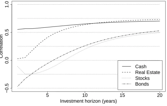
Therefore, we see again that the conditional covariance of the nominal asset return with inflation is crucial for the difference between the variance of real versus the variance of nominal returns. What we are missing to analyze the covariances are the horizon-dependent correlations of nominal asset returns with inflation, and these are shown in Figure 2.3. Cash is clearly the best inflation-hedging asset at short and medium horizons. Shocks to nominal cash returns are relatively highly correlated with inflation shocks and the correlation is increasing with the investment horizon.

At the twenty-year horizon, direct real estate appears to hedge inflation as well as cash. Bonds are the weakest inflation-hedging asset in the short term. In the long run, bonds and stocks have much better inflation-hedging abilities than in the short run.

There are theoretical arguments supporting this empirical evidence. Fama and Schwert (1977) point out that a strategy of rolling over short-term bills should offer a good hedge against longer-term unexpected inflation because short-term bill rates can adjust to reassessments of expected inflation. In contrast to this strategy, the cash-flows of a (default risk-free) nominal long-term bond are fixed, so the nominal long-term return does not move with inflation. Standard bond indexes, such as the one used in this paper, are, however, representing a security with constant matu- rity. In terms of inflation-hedging, this means that the return on these bond indexes benefits from the reassessments of expected inflation that are incorporated into the bond yield, so that the ability of constant maturity bond returns to hedge unex- pected inflation improves with the investment horizon. Campbell and Vuolteenaho (2004b) suggest that the finding of stocks being a perverse inflation-hedge in the short run, but a good inflation-hedge in the long run can be explained by money illusion. They find empirical support for the Modigliani and Cohn (1979) hypothe-

Figure 2.3: Conditional Correlations of Asset Returns and Inflation

5 10 15 20

−0.50.00.51.0

Investment horizon (years)

Correlation

Cash Real Estate Stocks Bonds

Notes: The figure shows conditional correlations of nominal returns and inflation depending on the investment horizon (years).

sis, who conclude that stock market investors suffer from a specific form of money illusion, disregarding the effect of changing inflation on cash-flow growth. When inflation rises unexpectedly, investors increase discount rates but ignore the impact of expected inflation on expected cash-flows, leading to an undervalued stock mar- ket, and vice versa. Because the mispricing should eventually diminish, stocks are a good inflation-hedge in the long run. Direct real estate has both stock and bond characteristics. Bond characteristics are due to the contractual rent representing a fixed-claim against the tenant. However, rents are routinely adjusted to market level through renting vacant space or arrangements in the lease contract. For example, in the UK commercial real estate market, contractual rents are usually reviewed every five years; they are adjusted to market-rent level when this level is above the contractual rent, otherwise the contractual rent remains unchanged. Thus, when general price and rent indexes are closely related, direct real estate should be a good long-term inflation hedge.

2.4.3 The Term Structure of Expected Returns

From Equations (2.9) and (2.11) one can calculate thek-period log expected nominal portfolio return as:

E

n^(k)_p,t+k + 1

2V ar

n^(k)_p,t+k

=E

n^(k)_0,t+k +1

2σ²₀(k) +α^′

E

x^(k)_t+k−c

+1

2σ_x²(k) +σ_0x(k)

. (2.14)

This equation shows how to calculate the approximation of the cumulative log ex- pected nominal portfolio return or, assuming a 100% investment in the respective asset, the log expected nominal return of any single asset class. Note that the ex- pected log return has to be adjusted by one half of the return variance to obtain the log expected return relevant for portfolio optimization (a Jensen’s inequality ad- justment); see Campbell and Viceira (2004). This adjustment is horizon-dependent.

There are no horizon effects in expected log returns because we assume that they take the values of their sample counterparts. Thus, for the k-period expected log nominal cash return it holds that E

n^(k)_0,t+k

=kn¯0 , where ¯n0 denotes the sample average of log nominal cash returns. Similarly, we assume for the vector of log ex- cess returns: E

x^(k)_t+k

=kx. Even if there were no horizon effects in expected log¯ returns, there would be horizon effects in log expected returns because conditional variances and covariances will not increase in proportion to the investment horizon unless returns are unpredictable. In the remainder of this paper, the log expected return is termed “expected return” for short.

Additional horizon effects in expected returns are due to the consideration of pro- portional transaction costs. With regard to stocks and bonds, transaction costs en- compass brokerage commissions and bid-ask spreads. Round-trip transaction costs for stocks are assumed to be 1%. Bid-ask spreads of government bonds are typically tiny; total round-trip transaction costs for bonds are assumed to be 0.1%. Transac- tion costs for buying and selling direct real estate encompass professional fees and the transfer tax. We assume round-trip transaction costs for direct real estate of 7%.

For a more extensive discussion about transaction costs of UK direct real estate we refer to Rehring (2012). The assumed round-trip transaction costs enter the vector c in continuously compounded form.

Table 2.3: Term Structure of Expected Returns Expected Returns p.a.

Real Returns Nominal Returns

Investment

1 5 10 20 1 5 10 20

Horizon

T-Bills 1.8% 1.9% 2.0% 2.1% 7.3% 7.4% 7.5% 7.7%

Real Estate -1.6% 3.4% 3.8% 4.1% 3.8% 8.9% 9.6% 10.1%

Stocks 6.9% 6.7% 6.8% 7.2% 12.4% 12.2% 12.3% 12.8%

Bonds 2.5% 2.5% 2.6% 2.6% 8.0% 7.9% 8.1% 8.2%

Notes: The table shows annualized expected real and nominal returns depending on the investment horizon (years). These follow from Equations (2.14) and (2.15), assuming a 100% investment in the respective asset. Expected log returns are assumed to equal their sample counterparts. Round-trip transaction costs are assumed to be 7.0% for real estate, 1.0% for stocks and 0.1% for bonds.

The k-period expected real portfolio return can be calculated from Equations (2.10) and (2.12) as:

E r_p,t+k^(k)

+ 1 2V ar

r^(k)_p,t+k

=E

n^(k)_0,t+k +1

2σ²₀(k)−E i^(k)_t+k

+1 2σ_i²(k) +α^′

E

x^(k)_t+k−c + 1

2σ²_x(k) +σ_0x(k)

(2.15)

−σ0i(k)−α^′σ_0x(k),

where E(it+k) =k¯i, the k-period expected log inflation and ¹₂σ_i²(k), one-half of the cumulative variance of inflation shocks, are common differences for the distinction between nominal expected returns and real expected returns for every asset. In addition, the conditional covariances between asset returns and inflation (σ0i(k) and σ_ix(k) respectively) play a role. The results of the comparison between the term structures of annualized expected real and nominal returns after transaction costs for cash, real estate, stocks, and bonds are shown in Table 2.3.

The difference between the expected real and nominal returns is a nearly parallel shift caused by the expected inflation. Due to transaction costs, there are major changes in the annualized expected direct real estate return, which increases strongly with the investment horizon, whereas the periodic expected returns on the other assets are roughly constant.

2.5 Horizon-Dependent Portfolio Optimizations

2.5.1 Mean-Variance Optimization

Campbell and Viceira (2002, 2004) provide the formula for the solution to the mean- variance problem. The optimization problem for nominal return is defined as:

max

α(k) E

n^(k)_p,t+k + 1

2(1−γ)V ar

n^(k)_p,t+k

. (2.16)

Augmented by transactions, we get the closed-form solution without any restrictions as:

α(k) = 1

γΣ⁻_xx¹(k)

E

x^(k)_t+k−c +1

2σ_x²(k)

+

1− 1 γ

−Σ⁻_xx¹(k)σ0x(k)

, (2.17) where γ is the coefficient of relative risk aversion. α(k) is a combination of two portfolios and the mixture depends on the investors risk aversion. The first portfolio:

Σ⁻_xx¹(k)

E

x^(k)_t+k−c +1

2σ_x²(k)

(2.18) is thegrowth optimal portfolio, the second portfolio is the global minimum variance portfolio and is the solution for an extreme risk averse investor (γ → ∞):

−Σ⁻_xx¹(k)σ0x(k). (2.19)

Formula (2.17) applies directly to the mean-variance problem for nominal returns.

The solution to the mean-variance problem for real returns differs from Equation (2.17) only by the definition of the global minimum variance portfolio, which is for real returns:

−Σ⁻_xx¹(k) (σ_0x(k)−σ_ix(k)). (2.20) We analyze two portfolios. One portfolio is the global minimum variance portfo- lio. The second portfolio represents a less risk-averse investor. Campbell and Viceira calculate a “tangency-portfolio” assuming the existence of a riskless asset. This is not suitable for our analysis, because we would have to assume that both real and nominal cash returns would be riskless (at any horizon) and hence there would be no inflation risk. Therefore, we calculate optimal horizon-dependent asset weights for a portfolio consisting of cash, bonds, stocks and direct real estate for a specific

coefficient of relative risk aversion; we chooseγ = 10. The necessary statistics can be calculated by applying appropriate selection matrices to Equations (2.6) and (2.8).

We rule out short-selling in both cases of the optimization. To get deeper insight into the shift effects we additionally calculate the portfolios for a non real estate investor denoted as base case.⁶

2.5.2 Results

Table 2.4 shows the two cases with optimal portfolio allocations for investment horizons of up to twenty years. Panel A reports the composition of the global minimum variance (GMV) portfolio for optimizations based on real and nominal returns. In the base case a very risk-averse investor holds all (real returns) or most (nominal returns) of his money in cash because it is the least risky investment in nominal as well as in real terms over all investment horizons. Bonds are more attractive in nominal than in real terms. Based on the optimizations for nominal returns, the weight increases from around 3% at the one-year horizon to 16% at the twenty-year horizon, whereas the weight is zero for all investment horizons when real returns are considered. Because of the hump shaped risk structure of nominal stock returns (high short and long-term volatility; less risky in the medium term), stocks get a small positive weight at medium investment horizons and get zero weight at long investment horizons.

Considering direct real estate as an additional asset the weight assigned to real estate is increasing with the investment horizon. The differences between the term structures of risk for nominal and real returns are crucial for the extent of the horizon effect. For the optimization based on nominal returns, the allocation to real estate increases up to 15% at long horizon. For real returns, the mean reversion effect is stronger and hence the weight assigned to real estate is much higher than the allocation for nominal returns at medium (35%) and long horizons (50%). Since the allocations for stocks and bonds remain nearly unchanged compared to the base case, the amount shifted to real estate arises mainly from a decreased cash allocation.

6We use the estimated VAR coefficients for the calculation and restrict the real estate weight to zero. Otherwise the results can be changed by different VAR estimates.

Table 2.4: Portfolio Calculations

Panel A Global Minimum Variance Portfolio Real Returns Nominal Returns Investment

1 5 10 20 1 5 10 20

Horizon Base Case

T-Bills 1.00 1.00 1.00 1.00 0.97 0.81 0.77 0.85 Stocks 0.00 0.00 0.00 0.00 0.00 0.06 0.04 0.00 Bonds 0.00 0.00 0.00 0.00 0.03 0.13 0.19 0.15 Direct Real Estate Investor

T-Bills 0.99 0.84 0.65 0.50 0.96 0.77 0.72 0.69 Real Estate 0.01 0.16 0.35 0.50 0.01 0.04 0.05 0.15 Stocks 0.00 0.00 0.00 0.00 0.00 0.05 0.04 0.00 Bonds 0.00 0.00 0.00 0.00 0.03 0.13 0.20 0.16 Panel B Optimal Portfolio Holdings forγ = 10

Real Returns Nominal Returns Investment

1 5 10 20 1 5 10 20

Horizon Base Case

T-Bills 0.86 0.73 0.60 0.47 0.85 0.56 0.33 0.42 Stocks 0.14 0.27 0.40 0.41 0.15 0.44 0.54 0.32 Bonds 0.00 0.00 0.00 0.12 0.00 0.00 0.13 0.26 Direct Real Estate Investor

T-Bills 0.86 0.48 0.00 0.00 0.85 0.43 0.00 0.00 Real Estate 0.00 0.29 0.66 0.75 0.00 0.15 0.36 0.64 Stocks 0.14 0.24 0.34 0.25 0.15 0.42 0.50 0.24 Bonds 0.00 0.00 0.00 0.00 0.00 0.00 0.15 0.13 Notes: The table shows optimal portfolio compositions for real and nominal returns depending on the investment horizon (years).

Panel B of Table 2.4 reports the portfolio allocations for an investor with risk aversion ofγ = 10. As noted above, we consider stocks, bonds, cash, and real estate in comparison to the base case where the investor is restricted to stocks, bonds, and cash. In addition to risk statistics, the term structures of expected returns are relevant for this portfolio. Recall that the differences with regard to nominal versus real returns are roughly parallel shifts. Hence, when comparing the results for nominal and real returns, the changing risk statistics are again crucial for the interpretation. We see once more that the differences in optimal portfolio weights are small at short horizons, since short-term return volatilities are similar for real and nominal returns. Due to the low expected return on real estate and the high volatility of stock returns, cash is the asset with the highest allocation at short horizons. The weight assigned to cash is strongly decreasing with the investment horizon. As in the GMV portfolio, direct real estate is much more attractive in the long run. Due to the short-selling restriction the allocation is zero at the one-year horizon. For a direct real estate investor the weight increases to 75% for real returns and to 64% for nominal returns at the twenty-year horizon, while the biggest differences between real and nominal real estate allocations is at the medium horizon (30 percentage points). For the optimization based on nominal returns, the allocation to stocks shows a hump-shaped structure with highest allocations (up to 54%) at intermediate horizons in both cases. For optimizations based on real returns, the allocations to stocks are smaller at medium horizons and the downward tilts for long horizons are less strong due to the strong mean reversion effect of real stock returns. The term structure of real bond returns is roughly flat and on a higher level than cash and real estate combined with a low expected return. Thus, bonds are of low importance in a portfolio based on real terms. In nominal terms, however, the weight assigned to bonds is increasing over longer investment horizons because stocks are getting very unattractive due to the increase in the periodic return volatility, which is stronger than the mean aversion of nominal bond returns over long horizons. Compared to the base case, direct real estate crowds out stocks, bonds and particularly cash.