Commercial Real Estate Investments and the Term Structure of Risk and Return

(1)

zu Immobilienökonomie und Immobilienrecht

Herausgeber:

IRE

I

BS International Real Estate Business School

Prof. Dr. Sven Bienert

Prof. Dr. Stephan Bone-Winkel Prof. Dr. Kristof Dascher Prof. Dr. Dr. Herbert Grziwotz Prof. Dr. Tobias Just

Prof. Dr. Kurt Klein

Prof. Dr. Jürgen Kühling, LL.M.

Prof. Gabriel Lee, Ph. D.

Prof. Dr. Gerit Mannsen

Prof. Dr. Dr. h.c. Joachim Möller Prof. Dr. Wolfgang Schäfers

Prof. Dr. Karl-Werner Schulte HonRICS Prof. Dr. Steffen Sebastian

Prof. Dr. Wolfgang Servatius Prof. Dr. Frank Stellmann Prof. Dr. Martin Wentz

Christian Rehring

Commercial Real Estate Investments and the Term Structure of

Risk and Return

(2)

Christian Rehring

Commercial Real Estate Investments

and the Term Structure of Risk and Return

(3)

Commercial Real Estate Investments and the Term Structure of Risk and Return Christian Rehring

Regensburg: Universitätsbibliothek Regensburg 2014

(Schriften zu Immobilienökonomie und Immobilienrecht; Bd. 68) Zugl.: Regensburg, Univ. Regensburg, Diss., 2010

ISBN 978-3-88246-341-5

© IRE|BS International Real Estate Business School, Universität Regensburg Verlag: Universitätsbibliothek Regensburg, Regensburg 2014

Zugleich: Dissertation zur Erlangung des Grades eines Doktors der Wirtschaftswissenschaften, eingereicht an der Fakultät für Wirtschaftswissenschaften der Universität Regensburg

Tag der mündlichen Prüfung: 15. Oktober 2010 Berichterstatter: Prof. Dr. Steffen Sebastian

Prof. Dr. Rolf Tschernig

(4)

Contents

List of Figures ... v

List of Tables ... vi

List of Abbreviations ... vii

List of Symbols ... ix

1 Introduction ... 1

2 Dynamics of Commercial Real Estate Asset Markets, Return Volatility, and the Investment Horizon ... 6

2.1 Introduction ... 7

2.2 Background and literature review ... 9

2.3 VAR model and data ... 12

2.3.1 VAR specification ... 12

2.3.2 Data ... 13

2.3.3 VAR estimates ... 17

2.4 Multi-period volatility and R² statistics ... 21

2.4.1 Methodology ... 21

2.4.2 Results ... 22

2.5 Variance decompositions ... 28

2.5.1 Methodology ... 28

2.5.2 Results ... 30

2.6 Market efficiency ... 33

2.7 Conclusion ... 36

2.8 Appendix: Data ... 37

3 Real Estate in a Mixed Asset Portfolio: The Role of the Investment Horizon... 38

3.2 Literature review ... 41

3.2.1 Return predictability and mixed asset allocation ... 41

3.2.2 Illiquidity and transaction costs ... 43

(5)

3.3.2 Data ... 45

3.4 Horizon effects in risk and return of ex post returns ... 51

3.4.1 The term structure of risk ... 51

3.4.2 The term structure of expected returns ... 55

3.5 The term structure of real estate’s ex ante return volatility ... 58

3.6 Horizon-dependent portfolio optimizations ... 62

3.6.1 Mean-variance optimization... 62

3.6.2 Mixed asset allocation results ... 62

3.6.3 The allocation to real estate under different asset allocation approaches ... 65

3.7 Robustness checks ... 68

3.7.1 Smoothing parameter ... 68

3.7.2 Quarterly dataset ... 70

3.9 Appendix A: Data ... 74

3.10 Appendix B: Approximation (3.10a) ... 75

4 Inflation-Hedging, Asset Allocation, and the Investment Horizon ... 77

4.2 Literature review ... 80

4.3.2 Data ... 84

4.4 Horizon effects in risk and return for nominal and real returns ... 90

4.4.1 The term structure of risk ... 90

4.4.2 Inflation hedging ... 94

4.4.3 The term structure of expected returns ... 99

4.5 Horizon-dependent portfolio optimizations for nominal and real returns .... 101

4.5.1 Mean-variance optimization... 101

4.5.2 Results ... 103

(6)

4.6 Robustness of the results with regard to the smoothing parameter ... 106

4.8 Appendix: Data ... 109

References ... 110

(7)

List of Figures

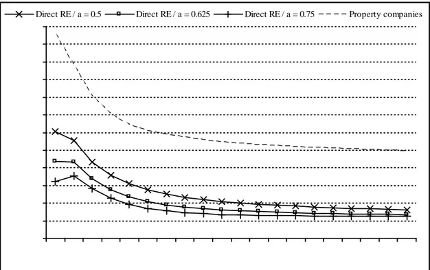
Figure 2.1 The term structure of return volatilities ... 24

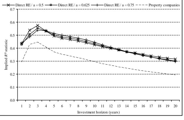
Figure 2.2 Implied R² statistics ... 27

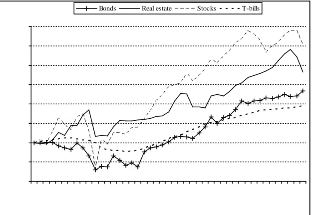
Figure 3.1 Total real return indexes ... 48

Figure 3.3 The term structure of return correlations ... 55

Figure 3.4 The term structure of expected returns ... 58

Figure 3.5 The term structure of real estate’s return volatility ... 60

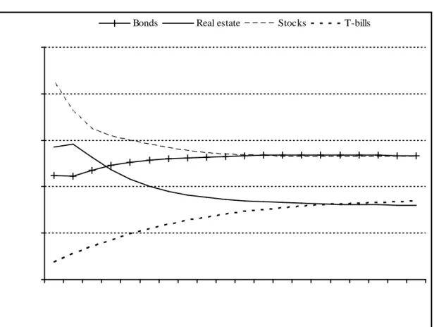
Figure 3.6 Optimal portfolio compositions ... 64

Figure 3.7 Real estate allocation under different asset allocation approaches ... 66

Figure 4.1 Total return and cost of living indexes ... 87

Figure 4.3 The term structure of return correlations ... 94

Figure 4.4 The term structure of inflation volatility ... 96

Figure 4.5 Inflation hedge properties ... 97

Figure 4.6 The term structure of expected returns ... 101

Figure 4.7 Optimal portfolio compositions ... 104

(8)

List of Tables

Table 2.1 Sample statistics ... 15

Table 2.2 Statistics of US direct real estate returns ... 16

Table 2.3 UK VAR results ... 18

Table 2.4 US VAR results ... 19

Table 2.5 Variance decompositions ... 31

Table 2.A1 Data information ... 37

Table 3.2 VAR results ... 49

Table 3.3 Results obtained from the use of alternative smoothing parameters ... 69

Table 3.4 Results obtained from quarterly dataset ... 72

Table 4.2 VAR results ... 88

Table 4.3 Results obtained from the use of alternative smoothing parameters ... 107

(9)

List of Abbreviations

AR Autoregressive CL Constant liquidity

e.g. for example (exempli gratia) excl. excluding

GDP Gross domestic product i.e. that is (id est)

IID Independently and identically distributed

IIDN Independently and identically normal distributed incl. including

IPD Investment Property Databank

MIT Massachusetts Institute of Technology MPRP Marketing period risk premium

NCREIF National Council of Real Estate Investment Fiduciaries NPI NCREIF Property Index

OLS Ordinary least squares p.a. per annum

RE Real estate

REIT Real estate investment trust St.dv. Standard deviation

TBI Transaction-Based Index VAR Vector autoregression VL Variable liquidity

(10)

UK United Kingdom US United States

(11)

List of Symbols

a Smoothing parameter c Vector of transaction costs

) (j

C j-th order autocovariance of the vector z_t+1 Corr(·) Correlation operator

Cov(·) Covariance operator

Covt(·) Conditional covariance operator CRt Cap rate at time t

CRUt Simple nominal capital return (unsmoothed) in period t CVt Capital value index at time t

diag(·) Diagonal of

d−p Mean log cash-payout-yield exp(·) Exponential operator

e1 Vector where the first element is one and the other elements are zero e2 Vector where the second element is one and the other elements are zero E(·) Expectation operator

Et(·) Conditional expectation operator f Mathematical function

gt True continuously compounded real capital return on real estate in period t g_t^* Appraisal-based continuously compounded real capital return on real estate in

period t

It+1 Inflation rate in period t+1

i_t+1 Continuously compounded inflation rate in period t+1

) (k

k

it₊ Continuously compounded k-period inflation rate

i Sample average of continuously compounded inflation rates I Identity matrix

Inc_t Real estate income in period t

IR_t Income return on real estate in period t IRUt

Income return on real estate with regard to unsmoothed capital value index in period t

(12)

j Index variable k Investment horizon

k* Period after which the marketing activities begin ln(·) Natural logarithm operator

m Marketing period Mn A selector matrix Mr A selector matrix

+1

nt Vector of continuously compounded nominal returns in period t+1

) (k t+k

n Vector of continuously compounded k-period nominal returns

1 , 0t+

n Continuously compounded nominal return on the benchmark asset in period +1

t

) (

, 0

k k

n t₊ Continuously compounded k-period nominal return on the benchmark asset

) (

, k

k t

np ₊ Continuously compounded k-period nominal portfolio return

n0 Sample average of continuously compounded nominal returns on the benchmark asset

p Order of vector autoregressive process P Persistence measure

j

rt₊₁₊ Continuously compounded real return in period t+1+ j

rt+1 Vector of continuously compounded real returns in period t+1

) (k t+k

r Vector of continuously compounded k-period real returns

r_0,t+1 Continuously compounded real return on the benchmark asset in period t+1

) (

, 0

k k

r t₊ Continuously compounded k-period real return on the benchmark asset

k t

rRE_,₊ Continuously compounded k-period real return on real estate, per period

) (

, k

k t

rp ₊ Continuously compounded k-period real portfolio return r0 Sample average of continuously compounded cash returns R_t+1 Nominal return in period t+1

R² Goodness of fit

RERt Total return on real estate in period t

s Slope of the term structure of the periodic expected real return on real estate s_t+1 Vector of state variables at time t+1

(13)

UCV_t Unsmoothed capital value index at time t vt+1 Vector of regression residuals at time t+1

) (k

V k-period matrix of total covariances of the vector zt+1

Var(·) Variance operator

Vart(·) Conditional variance operator Vec(·) Vec operator

W(k) Conditional k-period covariance matrix of the vector z_t

xt+1 Vector of continuously compounded excess returns in period t+1

) (k t+k

x Vector of continuously compounded k-period excess returns

x Vector of sample averages of continuously compounded excess returns zt+1 Vector of VAR-variables at time t+1

) (k

‡ Vector of asset weights with regard to a k-period investment horizon β Regression slope coefficient

+1

εt Residual of regression at time t+1 )

1(k

ϕt+ Cumulative (k-period) price adjustment γ Coefficient of relative risk aversion

+1

ηt Unexpected return in period t+1

j t+1+

η Innovations to future (period t+1+ j) expected returns

1 ,t+

ηd Cash-flow news in period t+1

1 ,t+

ηr Discount rate news in period t+1

Vector of ones

µp Continuously compounded expected real portfolio return, per period ρ Parameter of linearization

σ(·) Standard deviation operator )

2(

0 k

σ Variance of shocks to the k-period return on the benchmark asset )

2(

i k

σ Variance of shocks to the k-period inflation rate )

2(

x k

— Diagonal vector of xx with regard to horizon k )

0_i(k

σ Covariance of shocks to the k-period return on the benchmark asset with k- period inflation shocks

(14)

s

—0 Vector of covariances between shocks to the return on the benchmark asset and shocks to the state variables

)

0_x(k

σ Vector of covariances between shocks to the k-period return on the basis asset and shocks to the k-period excess returns on the other assets

)

in(k

σ Vector of covariances between k-period inflation shocks and shocks to k- period nominal returns

σis Vector of covariances between inflation shocks and shocks to the state variables

)

ix(k

σ Vector of covariances between shocks to k-period excess returns and k-period inflation shocks

∆dt+1+j Cash-flow growth in period t+1+ j

Σss Conditional covariance matrix of the state variables

î sx Conditional covariance matrix of excess returns and state variables Σv Covariance-matrix of regression residuals

)

xx(k

Σ Conditional covariance-matrix of k-period excess returns Φ Matrix of regression slope coefficients

Φ0 Vector of regression intercepts

Φ1 Matrix of regression slope coefficients ô Covariance matrix of VAR coefficients

(15)

1 Introduction

Although commercial real estate makes up for a large proportion of the world’s wealth, the analysis of real estate investments lags behind that of classic financial asset classes.

According to Clayton et al. (2009, p. 10), the lag of the application of insights from the finance literature to the investment analysis of commercial real estate can be seen as

“[…] one of the distinguishing features of the asset class.” They state:

“Many of the basic tools of portfolio management have now been applied to commercial real estate, but only in the last 10 to 15 years. The concepts may be 30, 40, or 50 years old, but institutional real estate investors have only just begun to use (and sometimes misuse) the standard techniques of the broader investment markets […].”

This thesis is devoted to the analysis of commercial real estate investments. The overall goal is to gain a better understanding of the financial characteristics of this asset class.

With an average holding period of about ten years, direct commercial real estate investments are typically long-term investments (Collet et al. 2003, Fisher and Young 2000). Motivated by this fact, the calculation of long-term risk and return statistics is at the heart of this thesis.

Following the tradition in real estate research, approaches originally applied to the traditional asset classes are applied to commercial real estate investments. A common characteristic of the models used in this thesis is to acknowledge that asset returns are predictable. Up to the 1980s, the common view was that stock and bond returns are (close to) unpredictable (Cochrane 2005, Chapter 20). Fama and Schwert (1977) were among the first to challenge the view of constant expected returns, emphasizing that expected stock returns vary with inflation. Since then, many other studies have shown that bond and stock returns are in fact predictable (e.g., Campbell 1987, Campbell and Shiller 1988, Fama 1984, and Fama and French 1988a, 1989). Research by Case and Shiller (1989, 1991), Gyourko and Keim (1992), Barkham and Geltner (1995) and Fu and Ng (2001), among others, shows that residential and commercial real estate returns are predictable, too.

(16)

When returns are predictable, there are horizon effects in periodic variances and covariances of multi-period returns – there is a „term structure of risk“. Consider a two- period example. Let rt+1 denote the log (continuously compounded) return in period

t+1, and rt+2 the log return in period t+2. Assuming that returns are identically distributed,

Var_t(r_t+1)+Var_t(r_t+2)=2Var_t(r_t+1)+2Cov_t(r_t+1,r_t+2) (1.1)

is the variance of the two-period return. When returns are unpredictable, the variance increases in proportion to the investment horizons. When returns are predictable, however, the periodic (dividing by two) variance of the two-period return is greater (mean aversion) or less (mean reversion) than the single-period return variance, depending on the covariance (Covt) of returns. Thus, mean aversion reflects a positive correlation between single-period returns, and mean reversion reflects negative autocorrelation. There is an important difference between unconditional and conditional variances of multi-period returns. Early studies on the long-term risk of stocks (Fama and French 1988b, Poterba and Summers 1988) examine horizon effects focusing on unconditional variances by analyzing the behavior of multi-period realized returns directly. In this thesis, conditional (indicated by the subscript t) variances of multi- period returns are analyzed throughout by using a multivariate time-series model – a vector-autoregression (VAR) – that captures time-variation in expected returns and yields implied estimates of variances of multi-period returns. Campbell (1991) emphasizes that ex post returns can be serially uncorrelated, although there are horizon effects in the conditional periodic variance of returns. Similar to horizon effects in (conditional) return variances, return predictability induces horizon effects in (conditional) multi-period covariances of the returns on different assets (see Campbell and Viceira 2004).

Predictability of returns also induces horizon effects in expected returns.¹ For example, the simple return, per period, decreases with the investment horizon when returns are mean-reverting. Assume that an asset, currently valued at 100, either increases or decreases by 10% with a probability of 50%. After two periods, the asset will be worth 121 with a probability of 25%, 99 with a probability of 50%, or 81 with a

1 See also Jurek and Viceira (2010) for a discussion.

(17)

probability of 25%, and the expected simple return is 0%. When returns are mean- reverting, the middle case will become more likely and the other cases will become less likely. In the extreme, there would be a 100% probability that the stock is worth 99, corresponding to a simple return of -1%, after two periods. Transaction costs induce additional horizon effects in expected returns. This has a large effect for the term structure of (periodic) expected returns on direct real estate, since transaction costs are very large compared to stock and bond investments.

With periodic variances, covariances and expected returns being horizon- dependent, the optimal asset allocation is horizon-dependent, too (Campbell and Viceira 2002, Chapter 2). This thesis focuses on the dependence of risk and return on the investment horizon. It rules out time-variation in risk. Chacko and Viceira (2005) analyze the importance of time-variation in stock market risk for the portfolio allocation of long-term investors. They conclude that changing risk does not induce large changes in the optimal allocation to stocks, because changes in risk are not very persistent.

Since the influential paper by Sims (1980), VARs have become a popular approach to analyze the dynamics of a set of variables in macroeconomics and finance, because “VARs are powerful tools for describing data and for generating reliable multivariate benchmark forecasts.” (Stock and Watson 2001, p. 113). It should be noted that the VAR coefficients might be biased. Stambaugh (1999) has shown that persistency of forecasting variables leads to biased estimates in univariate forecasting regressions in small samples, when innovations to returns and innovations to the forecasting variable are correlated. For example, the coefficient obtained from a regression of stock returns on the lagged dividend yield has an upward bias, because stock return and dividend yield residuals are highly negatively correlated. However, Ang and Bekaert (2007) find that in a bivariate regression the bias can be negative instead of positive. Hence, coefficients in multivariate regressions (which form a VAR model) might not be biased. In line with the bulk of the literature (e.g., Campbell and Viceira 2002, 2005, Campbell et al. 2003, Fugazza et al. 2007, Hoevenaars et al. 2008) no adjustments are made.

The specific characteristics of real estate asset markets make it necessary to be careful when models developed for classic financial assets are applied to the real estate market. Throughout the thesis, variables specific to the real estate market are incorporated in the VAR models to capture the dynamics of real estate returns adequately. As indicated above, transaction costs are considered for estimating the term

(18)

structure of expected returns. In Chapter 3, an aspect of the lack of liquidity of direct real estate investments – marketing period risk – is accounted for. A result of the specific microstructure of direct real estate asset markets is the lack of return indexes, which are comparable to stock and bond indexes. The available history of commercial real estate indexes is usually relatively short, and the indexes are subject to a range of biases. When analyzing direct real estate, appraisal-based returns are used (as it is common in real estate research). Appraisal-based returns are unsmoothed using the method proposed by Geltner (1993), which avoids the a priori assumption of uncorrelated true market returns, and robustness checks are conducted by recalculating main results with different parameter values used to unsmooth appraisal-based returns.² One of the implications of the use of indexes for direct real estate is that the results are more relevant for investors with a well-diversified portfolio than for investors holding only a few properties.³ It should be emphasized that the thesis focuses on commercial real estate. Some of the results may also apply to residential real estate, though, given the similarities between the dynamics of housing markets and commercial real estate markets (Gyourko 2009).

The remainder of this thesis consists of three self-contained chapters. In Chapter 2, the term structures of return volatility for UK and US direct and securitized commercial real estate are compared. The implications of the term structures of return volatility for the dependence of the degree of return predictability (R² statistics) on the investment horizon are examined. In order to get deeper insights into the term structures of return volatility, the variance of unexpected returns is decomposed into the variance of news about future cash flows, news about future returns and their covariance. A discussion of the informational efficiency of the asset markets is also part of this Chapter. Chapter 3 analyzes the role of the investment horizon for the allocation to UK direct commercial real estate in a mixed asset portfolio accounting for transactions costs, marketing period risk and return predictability. Furthermore, the chapter examines the relative importance of return predictability, transaction costs and marketing period risk for the optimal allocation to real estate. Chapter 4 analyzes how the inflation hedging abilities of UK cash, bond, stock and direct commercial real estate investments change with the investment horizon. The implications of the differing inflation hedge properties of the assets for the difference between the return volatility of

2 See Geltner et al. (2007, Chapter 25) for a textbook discussion of the data issues.

3 For a diversification analysis based on individual properties see Kallberg et al. (1996).

(19)

real returns versus the return volatility of nominal returns, and for portfolio choice are explored.

(20)

2 Dynamics of Commercial Real Estate Asset Markets, Return Volatility, and the Investment Horizon

This chapter is joint work with Steffen Sebastian.

Abstract

The term structure of return volatility is estimated for UK and US direct and securitized commercial real estate using vector autoregressions. To capture the dynamics of the real estate asset markets it is important to account for a valuation ratio specific to the asset market analyzed. In the UK, direct real estate and property shares exhibit mean reversion. US REIT returns are mean reverting, too. In contrast, US direct real estate shows a considerable mean aversion effect over short investment horizons. This can be explained by the positive correlation between cash-flow and discount rate news, which can be interpreted as underreaction to cash-flow news. In all of the asset markets analyzed, unexpected returns are primarily driven by news about discount rates. In the UK, direct real estate returns remain more predictable than property share returns in the medium and long term, whereas US REIT returns appear to be equally predictable to US direct real estate returns at a ten-year investment horizon.

(21)

2.1 Introduction

A lot of research in real estate focuses on the problem of how to correct (“unsmooth”) appraisal-based returns in order to obtain returns, which are closer to true market returns (e.g., Blundell and Ward 1987, Geltner 1993, Fisher et al. 1994). The unsmoothed returns are used to assess the volatility of real estate markets. The studies use quarterly or annual return data, however. Typically, real estate investors have longer investment horizons than a quarter or a year. With an average holding period of about ten years, direct commercial real estate investments are typically long-term investments (Collet et al. 2003, Fisher and Young 2000). The relationship between the short-term and the long-term return volatility is straightforward when returns are independently and identically distributed (IID) over time: The variance of (log) returns increases in proportion to the investment horizon. When returns are predictable, however, there may be substantial horizon effects in the periodic (divided by the square root of the investment horizon) volatility of returns. For example, there is a lot of evidence suggesting that stock returns are mean reverting, i.e., that the periodic long-term volatility of stock returns is lower than the short-term volatility.⁴

The widespread view is that commercial real estate returns are predictable.

Securitized real estate investments are often seen to exhibit similar dynamics as the general stock market. Conventional wisdom and empirical evidence (Clayton 1996, Geltner and Mei 1995, Scott and Judge 2000) suggest that direct real estate asset markets exhibit cyclicality. A series of high returns tends to be followed by a series of low returns, and vice versa. Hence, cyclicality implies that real estate returns are mean reverting over long investment horizons, making real estate relatively less risky in the long run. Cyclicality also implies that direct real estate exhibits return persistence over short investment horizons, so that we see mean aversion in the short run. The return persistence is typically attributed to the specific microstructure of the direct real estate asset market characterized by high transaction costs, low transaction frequency and heterogeneous goods, causing slow information diffusion (e.g., Geltner et al. 2007, Chapter 1). Thus, horizon effects in the volatility of returns are likely to be linked to the informational efficiency of an asset market.

4 Early references include Campbell (1991), Fama and French (1988a, 1988b), Kandel and Stambaugh (1987) and Porterba and Summers (1988).

(22)

The goal of this chapter is to analyze how important mean aversion and mean reversion effects are in UK and US direct and securitized commercial real estate markets. Using vector autoregressions (VARs), the term structure of the annualized return volatility is estimated for direct and securitized real estate in these two countries.

We explore the implications of the term structure of return volatility for the dependence of the degree of return predictability (R² statistics) on the investment horizon. In order to get deeper insights into the term structure of the return volatility of an asset, the variance of unexpected returns is decomposed into the variance of news about future cash flows, news about future returns, and their covariance.

We find that in the UK the results for direct real estate and property shares are similar to the results for the general stock market. Both UK direct and securitized real estate exhibit strong mean reversion. US REIT returns are strongly mean reverting, too.

In contrast, US direct real estate returns are considerably mean averting over short investment horizons, after which the term structure of the annualized volatility is slightly decreasing. To estimate the long-term return volatility of the assets adequately, it is important to include a valuation ratio specific to the asset market analyzed in the VAR models. The low short-term standard deviation and the mean aversion of US direct real estate returns can be explained by the positive correlation between cash-flow and discount rate news, which can be interpreted as underreaction to cash-flow news. In all of the asset markets analyzed, unexpected returns are primarily driven by news about discount rates. The choice of the parameter used to unsmooth appraisal-based returns has a large effect on the short-term, but not on the long-term volatility of direct real estate returns. In the UK, direct real estate returns remain more predictable than property share returns in the medium and long term, whereas US REIT returns appear to be equally predictable to US direct real estate returns at a ten-year investment horizon.

The remainder of the chapter is organized as follows: The next section contains a review of the literature and some background discussion. We proceed with a description of the VAR model and the data and present the VAR estimates. The next section contains the discussion of the term structure of return volatilities and the multi-period R² statistics implied by the VARs. The variance decompositions are presented in the subsequent section. A discussion and further analysis with regard to the informational efficiency of the real estate asset markets follows. The final section concludes the chapter.

(23)

2.2 Background and literature review

How does return predictability induce horizon effects in the periodic volatility of returns? To address this issue, most recent studies use VAR models. In this framework, risk is based on the unpredictable component of returns, i.e., the return variance is computed relative to the conditional return expectation. The conditional periodic volatility of multi-period returns can be calculated from the VAR results and may increase or decrease with the investment horizon. The standard example of horizon effects in the return volatility is the mean reversion effect in stock returns induced by the dividend yield. The dividend yield has been found to positively predict stock returns (Campbell and Shiller 1988, Fama and French 1988a). In combination with the large negative correlation between shocks to the dividend yield – whose process is usually well described by an AR(1) process – and shocks to the stock return, mean reversion in stock returns emerges: A low realized stock return tends to be accompanied by a positive shock to the dividend yield, and a high dividend yield predicts high stock returns for the future, and vice versa. Campbell and Viceira (2005) show that this effect cuts the periodic long-term standard deviation of US stock returns to approximately 50% of the short-term standard deviation. In general (see Campbell and Viceira 2004), returns exhibit mean reversion if the sign of the parameter obtained from a regression of an asset’s return on a lagged predictor variable has the opposite sign as the correlation between the contemporaneous shocks to the asset return and the predictor variable;

mean aversion is induced if the regression parameter and the correlation of the residuals are of the same sign. The higher the persistence of the forecasting variable, the more important is this predictor for the long-term asset risk.⁵

There are a lot of studies suggesting that commercial real estate returns are not IID. Direct real estate returns appear to be positively related to lagged stock returns (Quan and Titman 1999) and more specifically to the lagged returns on property shares (e.g., Gyourko and Keim 1992, Barkham and Geltner 1995). Furthermore, direct real estate returns appear to be positively autocorrelated over short horizons (Geltner 1993, Fu and Ng 2001). Fu and Ng (2001), Ghysels et al. (2007) and Plazzi et al. (2010) show that the cap rate predicts commercial real estate returns positively. (The cap rate of the

5 There is an additional effect, which always leads to an increase in the periodic conditional return variance. If the forecasting variable is very persistent, this effect – reflecting the variance of expected returns – may lead to a notable increase of the long-term return volatility, a point emphasized by Schotman et al. (2008).

(24)

real estate market is like the dividend yield of the stock market – the ratio of the income to the price of an asset.) Variables that have been used to predict REIT returns include the dividend yield of the general stock market, the cap rate of the direct real estate market and interest rate variables (e.g., Bharati and Gupta 1992, Liu and Mei 1992, 1994).

A few articles have looked at the implications of the predictability of commercial real estate returns for the term structure of return volatility. Geltner et al. (1995) calculate five-year risk statistics based on regressions of real estate returns on contemporaneous and lagged asset returns. These authors find that the variance of US private real estate returns at a five-year horizon is higher than five times the annual variance – reflecting mean-aversion. Using a VAR model, Porras Prado and Verbeek (2008) also find that US direct real estate exhibits mean aversion. Hence, the existing evidence points towards mean-aversion in direct US real estate returns.⁶ With regard to securitized real estate, the results are mixed. Fugazza et al. (2007) find that the standard deviation (per period) of European property shares is increasing with the investment horizon. Porras Prado and Verbeek (2008) find that returns of US property shares are mean averting. In contrast, Liu and Mei (1994) and Hoevenaars et al. (2008) find that US REIT returns exhibit mean-reversion, which is, however, weaker than the mean- reversion effect in the general stock market.

The VAR results can also be used to calculate the implied R² statistics of multi- period returns. Judging from regressions with quarterly or annual returns, direct real estate returns are more predictable than real estate share returns, but this may change with the investment horizon, because when expected returns are persistent, R² statistics can be much larger for longer horizons (Fama and French 1988a). Technically, persistence in expected returns makes the variance of expected multi-period returns increase faster than the total variance of multi-period returns. Chun et al. (2004) document rising R² statistics for US REITs over investment horizons of up to five years.

6 An exception is the article by MacKinnon and Al Zaman (2009), who find strong mean reversion in US direct real estate returns. The long-term (25-year) return volatility of real returns on direct real estate is estimated to be slightly below 2.0% per annum, identical to the estimated long-term stock return volatility. All of the asset classes analyzed by MacKinnon and Al Zaman – including US REITs – exhibit very strong mean reversion, though. For example, MacKinnon and Al Zaman find that the annualized 25-year volatility of US real cash returns is only 0.3%, compared to estimates of about 3% by Campbell and Viceira (2005), Hoevenaars et al. (2008) and Porras Prado and Verbeek (2008). Therefore, the results can be regarded as unusual.

(25)

Plazzi et al. (2010) find rising R² statistics over short investment horizons for US direct commercial real estate investments. More distant returns become less predictable, of course, so the R² statistics eventually decrease. Hence, we see a hump-shaped pattern of implied R² statistics in the general stock market (Kandel and Stambaugh 1987, Campbell 1991).

The variance of unexpected returns can be decomposed into the variance of news about future cash-flows, the variance of news about future returns (discount rates), and their covariance (Campbell 1991). This yields insights with regard to the return volatility. Discount rate news justify large changes in asset prices when expected returns are persistent. This mechanism induces mean reversion in returns: When discount rates increase, the price of the asset decreases, but expected returns are higher than before. In contrast, there is no such mechanism with regard to cash-flow news. Liu and Mei (1994) analyze US REITs and find that the variance of cash-flow news is larger than the variance of discount rate news, which results in a relatively weak mean-reversion effect, compared to the general stock market. Liu and Mei also find a positive correlation between cash-flow news and discount rate news, which attenuates the short-term return volatility. The reason is that positive cash-flow news increase prices, but positive discount rate news decrease prices. Though not employing Campbell’s (1991) variance decompositions, Geltner and Mei (1995) show that returns of US direct real estate investments are primarily driven by changing expected returns. In-sample forecasts of commercial real estate values track the market values closely when time-variation in discount rates is allowed for, whereas the forecasts are virtually constant over time and far removed from the actual market values when discount rates are held constant and only cash-flow forecasts are allowed to vary. Clayton (1996) analyzes the Canadian direct commercial real estate market and confirms the conclusion of Geltner and Mei that most of the volatility of direct real estate returns is caused by time-variation in discount rates.

In this chapter, we compare the UK and US direct and securitized real estate markets with regard to their term structure of return volatility. The comparison of the UK and the US market is particularly interesting with regard to the direct real estate market, because there is evidence that in the UK direct real estate market new information is timelier incorporated into prices than in the US. Specifically, annual appraisal-based US direct commercial real estate returns, unsmoothed with the Geltner (1993) method, still exhibit high autocorrelation, but in the case of the UK market,

(26)

returns are virtually uncorrelated after unsmoothing (Barkham and Geltner 1994).

Barkham and Geltner (1995) and Eichholtz and Hartzell (1996) find that in the UK direct real estate returns respond rather quickly to changes in securitized real estate returns, compared to the US. Thus, lag effects are more important in the US, whereas in the UK the contemporaneous relation between direct real estate and securitized real estate is stronger than in the US. For example, Barkham and Geltner (1995) find that the correlation between annual (unsmoothed) direct real estate returns and real estate stock returns is 61% in the UK, but only 19% in the US. These differences in the dynamics of the direct real estate markets should affect the term structure of the return volatility.

The high negative correlation between dividend yield and stock return residuals is crucial to capture mean reversion in stock returns (Campbell and Viceira 2005).

Therefore, we include common valuation ratios specific to real estate asset markets in the VAR models, whose residuals are highly negatively correlated with the return residuals. In particular, the cap rate of the direct real estate market is used to predict the return of the direct real estate market, and a valuation ratio specific to the market for securitized real estate is used as a return predictor for the securitized real estate market.

This point has been neglected by previous research on the term structure of the return volatility of real estate assets. (Previous studies on securitized real estate accounted for the dividend yield of the general stock market, but not for the dividend yield of the market for real estate stocks, or a similar valuation ratio specific to the real estate stocks market). Therefore, previous studies may have overestimated the long-term volatility of these assets. We link the results for the term structure of return volatilities to the variance decomposition of Campbell (1991), and use the VAR results to calculate multi- period R² statistics for real estate investments. Finally, we use the results of the variance decompositions to analyze the informational efficiency of the real estate asset markets.

2.3 VAR model and data 2.3.1 VAR specification

The results are based on separate VARs for each country using annual data from 1972 to 2008 (37 observations) for the UK market and from 1979 to 2008 (30 observations) for the US market.⁷ Let zt+1 be a (5x1) vector, whose first two elements are log

7 The main results for the UK market remain qualitatively unchanged, if the shorter time span 1979 to 2008 is used (as for the US market).

(27)

(continuously compounded) real asset returns, r_t₊₁ =ln(1+R_t₊₁)−ln(1+I_t₊₁), where Rt+1

is the simple nominal return on an asset and It+1 is the inflation rate. The first element of the vector zt+1 is the log real return on direct real estate; the second element is the log real return on securitized real estate. Asset returns are measured in real terms, since real rather than nominal returns are relevant for investors who are concerned about the purchasing power of their investments. Three additional state variables that predict the asset returns are included in zt+1. All variables are mean-adjusted. Assume that a VAR(1) model captures the dynamic relationships of the variables:⁸

1.

1 +

+ = _t + _t

t z v

z … (2.1)

… is a (5x5) coefficient-matrix. The shocks are stacked in the (5x1) vector vt+1 with time-invariant (5x5) covariance-matrix î _v.

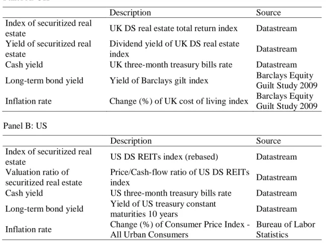
2.3.2 Data

To calculate the log real total return on securitized real estate, a property share index is used for the UK market and a REIT index is used for the US market. For the UK market the log of the dividend yield of the property share index is used as a state variable to predict the return on property shares. In analogy, we considered the dividend yield of the REIT market for the US VAR. However, this variable is not a significant predictor of REIT returns at any conventional levels. In contrast, another valuation ratio, the price to cash-flow ratio of the REIT market is a significant predictor of REIT returns. Hence, this variable is included as a state variable in the US VAR model in form of the log of the inverse of the variable, i.e., the log of the cash-flow yield. US REITs are restricted in their dividend policy since they have to pay out at least 90% (formerly 95%) of their taxable income as dividends. This restriction links the dividend payments of REITs to their earnings. Lamont (1998) shows with regard to the general stock market that in a univariate regression the earnings yield is not – in contrast to the dividend yield – a significant predictor of stock returns. This suggests that the dividend restriction of REITs might explain why the cash-flow to price ratio is a better valuation ratio to

8 The VAR(1) framework is not restrictive since a VAR(p) model can be written as a VAR(1) model, see Campbell and Shiller (1988).

(28)

forecast REIT returns than the dividend yield.⁹ We also include the yield spread as a state variable that has been shown to predict asset returns (e.g., Campbell 1987, Fama and French 1989). The variable is computed as the difference of the log yield on a long- term bond minus the log yield of three-month treasury bills. Details on the data can be found in the Appendix.

Appraisal-based capital and income returns are the basis for the calculation of the total return series and the cap rate series of direct real estate. The indexes used are the NCREIF property index (NPI) for the US market and the IPD long-term index for the UK market. The appraisal-based returns are unsmoothed using the approach introduced by Geltner (1993) for the US market and applied by Barkham and Geltner (1994) for the UK market. This unsmoothing approach does not presume that true real estate returns should be uncorrelated. Annual appraisal-based log real capital returns g_t^* are unsmoothed using the formula

g_t =g_t^*−(1−a)⋅g_t−1^*

a , (2.2)

where gt is the true log real capital return (or growth) and a is the smoothing parameter.

We use the value 0.40 (0.625) for unsmoothing annual US (UK) returns as favored by Geltner (1993) and Barkham and Geltner (1994), respectively. Total real estate returns and the cap rate series are constructed from the unsmoothed log real capital return and income return series as follows: The unsmoothed log real capital returns are converted to simple nominal capital returns (CRUt). This series is used to construct an unsmoothed capital value index (UCVt). The unsmoothed capital value index is calibrated such that the average of the capital values over time matches the corresponding average of the original index. A real estate income series (Inct) is obtained by multiplying the (original) income return (IRt) with the (original) capital value index (CV_t): Inc_t = IR_t⋅CV_t₋₁. New income returns are computed with regard to the unsmoothed capital value index: IRU_t =Inc_t/UCV_t₋₁. Total returns are obtained by adding the adjusted simple income and capital returns: RER_t =CRU_t +IRU_t. The cap

9 Chun et al. (2004) show that, after controlling for payout and book-to-market ratios, the price- dividend ratio is a significant predictor of excess US REIT returns.

(29)

rate series is calculated as CR_t =Inc_t /UCV_t. The variables included in the VAR are the log real total return, and the log of the cap rate.

As a robustness check for the UK market, we estimate additional VARs based on direct real estate return and cap rate series that result from using the smoothing parameters 0.50 and 0.75, which Barkham and Geltner (1994) consider as reasonable lower and upper bounds. In analogy, US results are recalculated for the alternative smoothing parameters 0.33 and 0.50 following Geltner (1993). To save space, we provide only the results concerning direct real estate from these additional VAR estimates, since the results for securitized real estate and the three state variables are not much affected by using the different real estate return and cap rate series resulting from the alternative smoothing parameters in the VARs.

Table 2.1 lists the standard deviations and first-order autocorrelations of the variables included in the benchmark UK VAR (a = 0.625) and the benchmark US VAR (a = 0.40). Direct real estate returns are much more volatile in the UK than in the US, and the UK returns exhibit less autocorrelation than the US returns. The returns of securitized real estate investments are also more volatile in the UK compared to the US.

The additional three state variables all show notable positive autocorrelation.

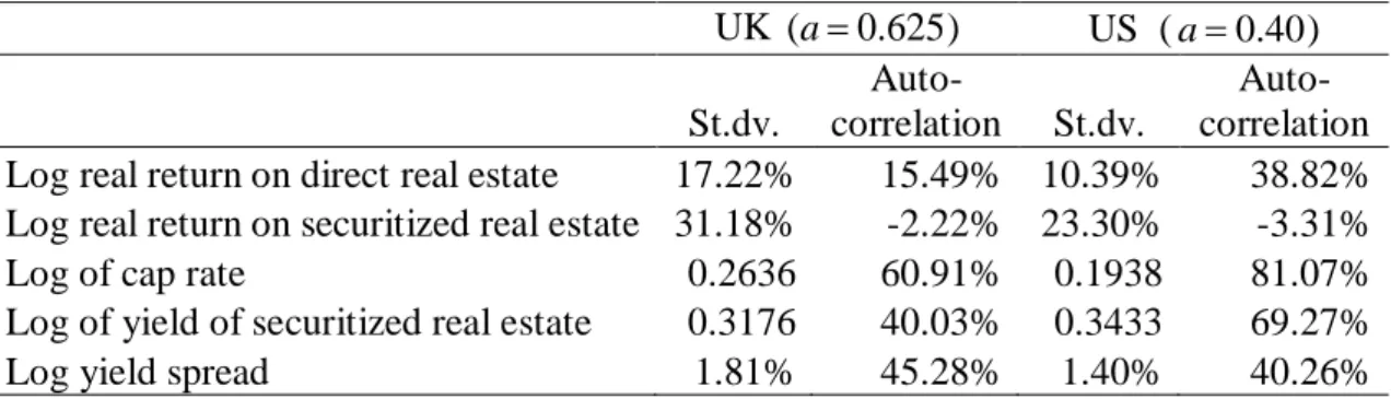
Table 2.1 Sample statistics

This table shows statistics for the variables included in the VAR models, which are based on annual data. The sample period is 1972 to 2008 for the UK. The US sample period is 1979 to 2008. Direct real estate return and cap rate statistics are based on the smoothing parameter (a) 0.625 for the UK and 0.40 for the US. St.dv.: Standard deviation. Autocorrelation refers to the first-order autocorrelation.

UK (a=0.625) US (a=0.40) St.dv.

Auto-

correlation St.dv.

Auto- correlation Log real return on direct real estate 17.22% 15.49% 10.39% 38.82%

Log real return on securitized real estate 31.18% -2.22% 23.30% -3.31%

Log of cap rate 0.2636 60.91% 0.1938 81.07%

Log of yield of securitized real estate 0.3176 40.03% 0.3433 69.27%

Log yield spread 1.81% 45.28% 1.40% 40.26%

Since the Center for Real Estate at MIT provides the Transaction-Based Index (TBI) for the US commercial real estate market, one might object the use of (unsmoothed) appraisal-based returns. The TBI is based on property transactions in the pool of properties that are used to construct the appraisal-based NPI (for details on the

(30)

construction of the TBI see Fisher et al. 2007). It should be emphasized, however, that, while transaction-based indexes have the advantage to be based on transaction prices (instead of appraisal), they are not generally preferable to (unsmoothed) appraisal-based indexes, because they might be subject to other problems such as noise due to the relatively small amount of property transactions (in contrast to appraisals).¹⁰ The NPI index has the advantage that it goes back further in time than the TBI. Nevertheless, to see how the unsmoothed NPI returns used in this chapter compare to TBI returns, Table 2.2 provides some statistics of unsmoothed NPI and TBI returns for the period of overlap 1985 to 2008. TBI returns are reported for both the variable and the constant liquidity version of the TBI. (We compare appreciation returns instead of total returns, since the constant liquidity version is available as an appreciation return index only.) The construction of a constant liquidity transaction-based index is motivated by the fact that liquidity is time-varying and pro-cyclical in real estate markets (see Fisher et al.

2003 and Goetzmann and Peng 2006). While the variable liquidity TBI tracks the development of transaction prices in the commercial real estate markets, it reflects variable market liquidity. The constant liquidity TBI is an index that tracks the development of transaction prices under the assumption of constant liquidity.

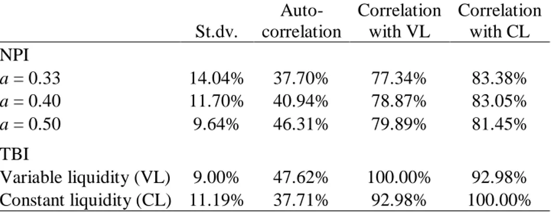
Table 2.2 Statistics of US direct real estate returns

This table shows statistics of mean-adjusted log real capital returns, based on annual data from 1985 to 2008. Unsmoothed NPI return statistics are reported for three smoothing parameters a. TBI return statistics are reported for the variable liquidity (VL) and the constant liquidity (CL) version. St.dv.: Standard deviation. Autocorrelation refers to the first-order autocorrelation.

St.dv.

Auto- correlation

Correlation with VL

Correlation with CL NPI

a = 0.33 14.04% 37.70% 77.34% 83.38%

a = 0.40 11.70% 40.94% 78.87% 83.05%

a = 0.50 9.64% 46.31% 79.89% 81.45%

TBI

Variable liquidity (VL) 9.00% 47.62% 100.00% 92.98%

Constant liquidity (CL) 11.19% 37.71% 92.98% 100.00%

10 See Geltner et al. (2007, Chapter 25) for a discussion of appraisal-based and transaction-based commercial real estate indexes.

(31)

As can be seen in Table 2.2, the constant liquidity returns show a higher volatility and lower autocorrelation than the variable liquidity returns. Unsmoothed NPI returns have correlations with TBI returns of about 80%, and the correlations are generally higher with regard to the constant liquidity version of the TBI than with the variable liquidity version. This is consistent with the view of Fisher et al. (1994, 2003) that unsmoothing procedures can be seen as an attempt to control for pro-cyclical variable liquidity.

Constant liquidity returns are better comparable to stock returns, since well-developed stock markets offer (approximately) constant liquidity. Judging from the return standard deviations, the smoothing parameter a=0.40 favored by Geltner (1993) indeed appears to be more reasonable than the values 0.33 and 0.50. Annual TBI returns show a similar autocorrelation as unsmoothed appraisal-based returns. Hence, the notable autocorrelation in annual returns of about 40% indeed seems to be a feature of the direct US real estate market.

2.3.3 VAR estimates

The results of the VARs, estimated by OLS, are given in Tables 2.3 (UK) and 2.4 (US).

Panels A contain the coefficients. In square brackets are t-values. The rightmost column contains R² statistics and the p-value of the F-test of joint significance (in parentheses).

With R² values of about 29 and 35% the degree of predictability of annual securitized real estate returns is similar in the two countries. With an R² value of 60%, US direct real estate returns are much more predictable than US REIT returns and UK direct and securitized real estate returns. Direct real estate has a higher R² value than securitized real estate in the UK as well. The p-values of the test of joint significance are below or close to 5% and thus indicate that real returns of direct and securitized real estate are indeed predictable in both countries.

(32)

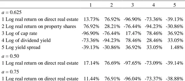
Table 2.3 UK VAR results

The results are based on mean-adjusted annual data from 1972 to 2008. Full VAR results are reported for the smoothing parameter a = 0.625, and VAR results concerning only direct real estate are reported for a = 0.50 and a = 0.75. Panel A shows the VAR coefficients. The t-statistics are in square brackets; values corresponding to p-values of 10% or below are highlighted. The rightmost column contains the R² values and the p- value of the F-test of joint significance in parentheses. Panel B shows results regarding the covariance matrix of residuals, where standard deviations are on the diagonal and correlations are on the off-diagonals.

Panel A: VAR coefficients

Coefficients on lagged variables

R² (p)

Variable 1 2 3 4 5

a = 0.625

1 Log real return on direct real estate 0.199 0.162 0.323 0.016 2.180 42.82%

[0.858] [1.177] [2.414] [0.122] [1.590] (0.28%) 2 Log real return on property shares 0.105 0.161 0.344 0.336 2.109 29.24%

[0.219] [0.569] [1.251] [1.240] [0.748] (4.72%) 3 Log of cap rate -0.087 -0.224 0.600 0.024 -4.594 57.06%

[-0.295] [-1.280] [3.520] [0.140] [-2.632] (0.00%) 4 Log of dividend yield -0.065 -0.027 -0.334 0.622 -4.054 26.81%

[-0.134] [-0.095] [-1.204] [2.271] [-1.426] (7.04%) 5 Log yield spread 0.012 -0.032 0.004 0.001 0.460 42.66%

[0.461] [-2.182] [0.243] [0.086] [3.118] (0.29%)

a = 0.50

[0.564] [1.196] [2.452] [0.147] [1.612] (0.23%)

a = 0.75

[1.269] [1.199] [2.419] [0.124] [1.585] (0.22%)

Panel B: Standard deviations and correlations of VAR residuals

1 2 3 4 5

a = 0.625

1 Log real return on direct real estate 13.73% 76.92% -96.90% -73.36% -39.13%

2 Log real return on property shares 76.92% 28.21% -76.44% -94.23% -30.86%

3 Log of cap rate -96.90% -76.44% 17.47% 78.46% 36.92%

4 Log of dividend yield -73.36% -94.23% 78.46% 28.46% 33.05%

5 Log yield spread -39.13% -30.86% 36.92% 33.05% 1.48%

a = 0.50

a = 0.75

(33)

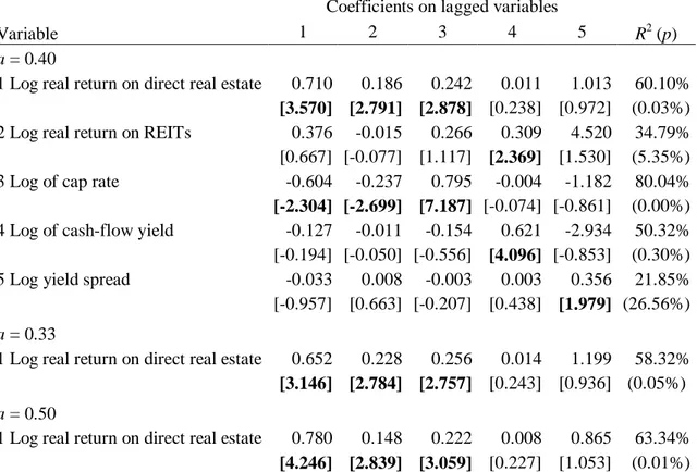
Table 2.4 US VAR results

The results are based on mean-adjusted annual data from 1979 to 2008. Full VAR results are reported for the smoothing parameter a = 0.40, and VAR results concerning only direct real estate also reported for a = 0.33 and a = 0.50. Panel A shows the VAR coefficients. The t-statistics are in square brackets; values corresponding to p-values of 10% or below are highlighted. The rightmost column contains the R² values and the p- value of the F-test of joint significance in parentheses. Panel B shows results regarding the covariance matrix of residuals, where standard deviations are on the diagonal and correlations are on the off-diagonals.

Panel A: VAR coefficients

Coefficients on lagged variables

R² (p)

Variable 1 2 3 4 5

a = 0.40

[3.570] [2.791] [2.878] [0.238] [0.972] (0.03%) 2 Log real return on REITs 0.376 -0.015 0.266 0.309 4.520 34.79%

[0.667] [-0.077] [1.117] [2.369] [1.530] (5.35%) 3 Log of cap rate -0.604 -0.237 0.795 -0.004 -1.182 80.04%

[-2.304] [-2.699] [7.187] [-0.074] [-0.861] (0.00%) 4 Log of cash-flow yield -0.127 -0.011 -0.154 0.621 -2.934 50.32%

[-0.194] [-0.050] [-0.556] [4.096] [-0.853] (0.30%) 5 Log yield spread -0.033 0.008 -0.003 0.003 0.356 21.85%

[-0.957] [0.663] [-0.207] [0.438] [1.979] (26.56%)

a = 0.33

[3.146] [2.784] [2.757] [0.243] [0.936] (0.05%)

a = 0.50

[4.246] [2.839] [3.059] [0.227] [1.053] (0.01%)

Panel B: Standard deviations and correlations of VAR residuals

1 2 3 4 5

a = 0.40

2 Log real return on REITs 51.30% 20.34% -36.69% -87.12% -27.10%

3 Log of cap rate -90.31% -36.69% 9.45% 32.15% 44.55%

4 Log of cash-flow yield -38.23% -87.12% 32.15% 23.67% 18.36%

5 Log yield spread -49.89% -27.10% 44.55% 18.36% 1.24%

a = 0.33

a = 0.50

(34)

The dynamics of real estate returns in the UK and in the US are qualitatively similar.

But there are notable differences with regard to the magnitude and significance of some coefficients. In particular, direct real estate returns in the US strongly depend positively and significantly on its own lag, which is not the case for direct real estate in the UK.

The return on securitized real estate has a positive influence on direct real estate returns in both countries, but the influence is not significant in the UK. Direct real estate returns are significantly affected by the lagged cap rate in both countries. The lagged cap rate also has a positive (though not significant) influence on securitized real estate returns.

The lagged dividend/cash-flow yield of the securitized real estate markets has a positive influence on securitized real estate returns. The coefficient is not significant in the UK, but in a regression of property share returns on the lagged dividend yield alone this is the case (t-value of 2.75). Finally, the lagged yield spread is positively related to direct and securitized real estate returns. The coefficients are never significantly different from zero at the 10% level, though. All three additional state variables show persistent behavior with coefficients on their own lags of between 0.356 and 0.795. Since these state variables predict asset returns, the persistency of the state variables carries over to expected asset returns, making expected returns positively autocorrelated. A shock to the expected return persists for some periods ahead, but eventually dies out. The dynamics of some of the state variables are more complex, however. In the UK, the lagged yield spread is also a significant predictor of the cap rate. In the US, lagged direct real estate returns and REIT returns have a significantly negative influence on the cap rate. Due to the positive autocorrelation in direct real estate returns, a price increase of direct real estate in period t−1 tends to be associated with a price increase in t, which lowers the cap rate in t. Similarly, the dependence of the cap rate on the lagged REIT return can be explained by the dependence of direct real estate returns on lagged REIT returns. The dynamics are very similar, when the results are based on the alternative smoothing parameter assumptions.

Panels B of Tables 2.3 and 2.4 contain the standard deviations (diagonal) and correlations (off-diagonals) of the VAR residuals. We see that the standard deviation of direct real estate return residuals is much lower in the US than in the UK. There are two reasons for this result. First, the total return variance is lower in the US, as seen in Table 2.1. Second, annual direct real estate returns are more predictable in the US, which means that the unexpected part of the total variance is smaller. The choice of the smoothing parameter has a notable influence on the residual standard deviation of UK