Optimal Asset Allocation under Quadratic Loss Aversion

IHS Economics Series Working Paper 291

September 2012

Optimal Asset Allocation under Quadratic Loss Aversion

Ines Fortin

Jaroslava Hlouskova

Impressum Author(s):

Ines Fortin, Jaroslava Hlouskova Title:

Optimal Asset Allocation under Quadratic Loss Aversion ISSN: Unspecified

2012 Institut für Höhere Studien - Institute for Advanced Studies (IHS) Josefstädter Straße 39, A-1080 Wien

E-Mail: o ce@ihs.ac.atffi Web: ww w .ihs.ac. a t

All IHS Working Papers are available online: http://irihs. ihs. ac.at/view/ihs_series/

This paper is available for download without charge at:

https://irihs.ihs.ac.at/id/eprint/2161/

Optimal Asset Allocation under Quadratic Loss Aversion

Ines Fortin, Jaroslava Hlouskova

291

Reihe Ökonomie

Economics Series

291 Reihe Ökonomie Economics Series

Optimal Asset Allocation under Quadratic Loss Aversion

Ines Fortin, Jaroslava Hlouskova September 2012

Institut für Höhere Studien (IHS), Wien

Contact:

Ines Fortin

Department of Economics and Finance Institute for Advanced Studies Stumpergasse 56

1060 Vienna, Austria

: +43/1/599 91-165 email: fortin@ihs.ac.at Jaroslava Hlouskova

Department of Economics and Finance Institute for Advanced Studies Stumpbergasse 56

1060 Vienna, Austria

: +43/1/599 91-142 email: hlouskov@ihs.ac.at and Thompson Rivers University School of Business and Economics Kamloops, British Columbia, Canada

Founded in 1963 by two prominent Austrians living in exile – the sociologist Paul F. Lazarsfeld and the economist Oskar Morgenstern – with the financial support from the Ford Foundation, the Austrian Federal Ministry of Education and the City of Vienna, the Institute for Advanced Studies (IHS) is the first institution for postgraduate education and research in economics and the social sciences in Austria. The Economics Series presents research done at the Department of Economics and Finance and aims to share “work in progress” in a timely way before formal publication. As usual, authors bear full responsibility for the content of their contributions.

Das Institut für Höhere Studien (IHS) wurde im Jahr 1963 von zwei prominenten Exilösterreichern – dem Soziologen Paul F. Lazarsfeld und dem Ökonomen Oskar Morgenstern – mit Hilfe der Ford- Stiftung, des Österreichischen Bundesministeriums für Unterricht und der Stadt Wien gegründet und ist somit die erste nachuniversitäre Lehr- und Forschungsstätte für die Sozial- und Wirtschafts- wissenschaften in Österreich. Die Reihe Ökonomie bietet Einblick in die Forschungsarbeit der Abteilung für Ökonomie und Finanzwirtschaft und verfolgt das Ziel, abteilungsinterne Diskussionsbeiträge einer breiteren fachinternen Öffentlichkeit zugänglich zu machen. Die inhaltliche Verantwortung für die veröffentlichten Beiträge liegt bei den Autoren und Autorinnen.

Abstract

We study the asset allocation of a quadratic loss-averse (QLA) investor and derive conditions under which the QLA problem is equivalent to the mean-variance (MV) and conditional value-at-risk (CVaR) problems. Then we solve analytically the two-asset problem of the QLA investor for a risk-free and a risky asset. We find that the optimal QLA investment in the risky asset is finite, strictly positive and is minimal with respect to the reference point for a value strictly larger than the risk-free rate. Finally, we implement the trading strategy of a QLA investor who reallocates her portfolio on a monthly basis using 13 EU and US assets.

We find that QLA portfolios (mostly) outperform MV and CVaR portfolios and that incorporating a conservative dynamic update of the QLA parameters improves the performance of QLA portfolios. Compared with linear loss-averse portfolios, QLA portfolios display significantly less risk but they also yield lower returns.

Keywords

Quadratic loss aversion, prospect theory, portfolio optimization, MV and CVaR portfolios, investment strategy

JEL Classification

D03, D81, G11, G15, G24

Comments

This research was supported by funds of the Oesterreichische Nationalbank (Anniversary Fund, Grant

Contents

1 Introduction 1

2 Portfolio optimization under quadratic loss aversion 3

2.1 Quadratic loss-averse utility versus mean-variance and conditional value-at-Risk .... 4 2.2 Analytical solution for one risk-free and one risky asset ... 8 2.3 Numerical solution ... 19

3 Empirical application 20

4 Conclusion 31

Appendix A 33

Appendix B 38

References 43

1 Introduction

Loss aversion, which is a central finding of Kahneman and Tversky’s (1979) prospect theory,¹ describes the fact that people are more sensitive to losses than to gains, relative to a given reference point. More specifically returns are measured relative to a given reference value, and the decrease in utility implied by a marginal loss (relative to the reference point) is always greater than the increase in utility implied by a marginal gain (relative to the reference point).² The simplest form of such loss aversion is linear loss aversion, where the marginal utility of gains and losses is fixed.

The optimal asset allocation decision under linear loss aversion has been extensively studied, see, for example, Gomes (2005), Siegmann and Lucas (2005), He and Zhou (2011), and Fortin and Hlouskova (2011a). It has been argued, however, that real investors may put an increasing rather than a fixed marginal penalty on losses, i.e., investors could be more averse to larger than to small losses. Thus a quadratic form of loss aversion, where the objective is linear in gains and quadratic in losses, may be more adequate. Quadratic loss aversion differs from the originally introduced (S-shaped) loss aversion in that it displays risk-aversion in both domains of gains and losses, while prospect theory (S-shaped) utility captures a risk-averse behavior in the domain of gains and a risk-seeking behavior in the domain of losses. Under quadratic loss aversion, investors face a trade- off between return on the one hand and quadratic shortfall below the reference point on the other hand. Interpreted differently, the utility function contains an asymmetric or downside risk measure, where losses are weighted differently from gains. Compared with linear loss aversion, large losses are punished more severely than small losses under quadratic loss aversion. The penalty on losses under quadratic loss aversion is also referred to as quadratic shortfall (see Siegmann and Lucas, 2005; Siegmann, 2007; and Lucas and Siegmann, 2008). Very recently, the analysis of optimal investment with capital income taxation under loss-averse preferences was conducted in Hlouskova and Tsigaris (2012). Some results indicate that it could be possible for a capital income tax increase not to stimulate risk taking even if the tax code provides the attractive full loss offset provisions.

However, risk taking can be stimulated if the investor interprets part of the tax as a loss instead of as a reduced gain.

1Sometimes the different versions of prospect theory are classified as three generations of prospect theory. The first generation builds on the original model introduced in Kahneman and Tversky (1979), the second generation (cumulative prospective theory) features cumulative individual probabilities (see, e.g., Tversky and Kahneman, 1992), and the third generation treats the reference point as being uncertain (see Schmidt, Starmer and Sugden, 2008).

2This is also referred to as the first-order risk aversion (see Epstein and Zin, 1990).

Asymmetric – or rather downside – risk measures are extremely popular in applied finance, where their use has been promoted by banking supervisory regulations which specify the risk of proprietary trading books and its use in setting risk capital requirements. The measure of risk used in this framework is value-at-risk (VaR), which explicitly targets downside risk, see the Bank for International Settlements (2006, 2010). VaR has been developing into one of the industry stan- dards for assessing the risk of financial losses in risk management and asset/liability management.

Another risk measure, which is closely related to VaR but offers additional desirable properties like information on extreme events, coherence and computational ease, is conditional value-at-risk (CVaR).³ Computational optimization of CVaR is readily accessible through the results in Rock- afellar and Uryasev (2000).

The purpose of this paper is to investigate the asset allocation decision under quadratic loss aver- sion, both theoretically and empirically, and compare it to more traditional portfolio optimization methods like mean-variance and conditional value-at-risk as well as to the recent asset allocation problem under linear loss aversion. Our theoretical analysis of the problem under quadratic loss aversion is related to Siegmann and Lucas (2005) who mainly explore optimal portfolio selection under linear loss aversion and include a brief analysis on quadratic loss aversion.⁴ Their setup, how- ever, is in terms of wealth (while our analysis is based on returns) and they characterize the solution in a different way than we do. We contribute to the existing literature along different lines. First, we investigate theoretically how the optimization problems of quadratic loss aversion, mean-variance and CVaR relate to each other. Second, we analytically solve the portfolio selection problem of a quadratic loss-averse investor and compare the results to those implied by linear loss aversion.

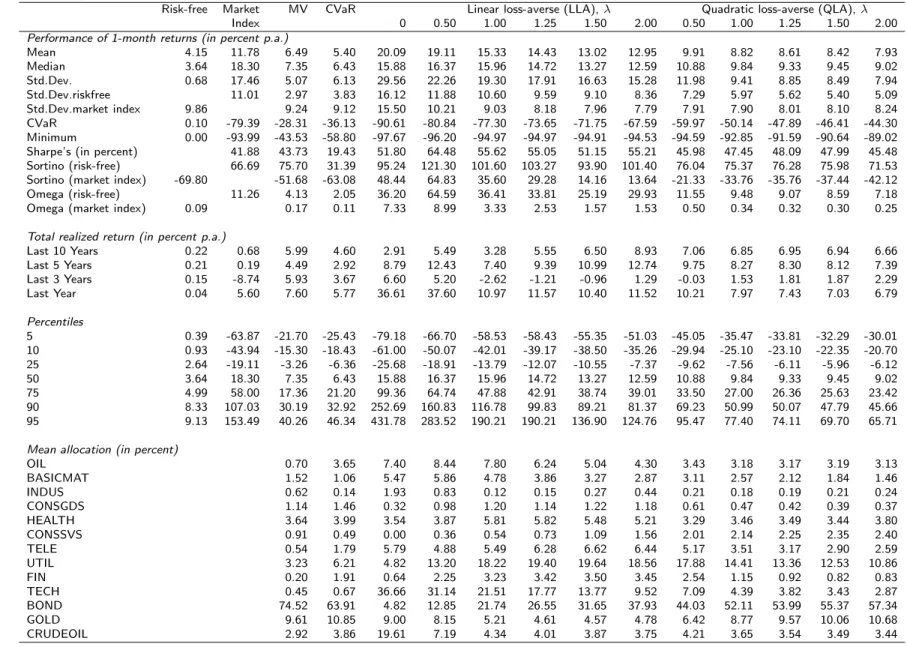
Third, we contribute to the empirical research involving loss-averse investors by investigating the portfolio performance under the optimal investment strategy, where the portfolio is reallocated on a monthly basis using 13 European and 13 US assets from 1985 to 2010. In addition to using fixed parameters in the loss-averse utility, we employ time-changing trading strategies which depend on previous gains and losses to better reflect the behavior of real investors. As opposed to a number of other authors, we do not consider a general equilibrium model but examine the portfolio selection problem from an investor’s point of view.⁵

3See Artzner et al. (1999).

4Siegmann and Lucas (2005) refer to what we call linear and quadratic loss aversion as linear and quadratic shortfall, respectively.

5See, for example, De Giorgi and Hens (2006) who introduce a piecewise negative exponential function as the loss-averse utility to overcome infinite short-selling and to guarantee the existence of market equilibria and Berkelaar

The remaining paper is organized as follows. In Section 2 we first derive conditions under which the quadratic loss-averse (QLA) utility maximization problem is equivalent to the traditional mean- variance (MV) and conditional value-at-risk (CVaR) problems for the general n-asset case, under the assumption of normally distributed asset returns. Then we explore the two-asset case, where one asset is risk-free, and derive properties of the optimal weight of the risky asset under the assumption of binomially and (generally) continuously distributed returns, both for the case when the reference point is equal to the risk-free rate and for the case when it is not. We additionally contrast the derived results with those implied by linear loss aversion (LLA). In Section 3 we implement the trading strategy of a quadratic loss-averse investor, who reallocates her portfolio on a monthly basis, and study the performance of the resulting optimal portfolio. We also compare the optimal QLA portfolio to the optimal LLA portfolio and to the more traditional optimal MV and CVaR portfolios. Section 4 concludes.

2 Portfolio optimization under quadratic loss aversion

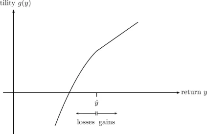
Under quadratic loss aversion investors are characterized by a utility of returns,g(·), which is linear in gains and quadratic in losses, where gains and losses are defined relative to a given reference point. Formally, g(y) = y−λ([ˆy−y]⁺)², where y is the (portfolio/asset) return,λ≥0 is the loss aversion – or penalty – parameter, ˆy ∈R is the reference point that defines gains and losses, and [t]⁺ denotes the maximum of 0 and t. See Figure 1 for a graphical illustration of the quadratic loss-averse utility. Compared with linear loss aversion, large losses are punished more severely than small losses under quadratic loss aversion.

We start by studying the optimal asset allocation behavior of a quadratic loss-averse investor.

This behavior depends on the reference return ˆyand, in particular, on whether this reference return is below, equal to, or above the (requested lower bound on the) expected portfolio return or some threshold value that is larger than the risk-free interest rate. Investors maximize their expected utility of returns as

maxx

n

E r^′x−λ([ˆy−r^′x]⁺)²

Ax≤b o

(2.1)

and Kouwenberg (2009) who analyze the impact of loss-averse investors on asset prices.

wherex= (x₁, . . . , x_n)^′,withx_i denoting the proportion of wealth invested in asseti,⁶ i= 1, . . . , n, andris then−dimensional random vector of returns, subject to the usual asset constraintsAx≤b, where A ∈ R^m×n, b ∈R^m. Note that in general the proportion invested in a given asset may be negative or larger than one due to short-selling.

ˆ y

returny utilityg(y)

gains losses

Figure 1: Quadratic loss-averse utility function

2.1 Quadratic loss-averse utility versus mean-variance and conditional value- at-risk

In this section we show the relationship between the quadratic loss-averse utility maximization prob- lem (2.1) and both the MV and the CVaR problems, under the assumption of normally distributed asset returns.⁷

LetZ be a continuous random variable describing the stochastic portfolio return andf_Z(·) and F_Z(·) be its probability density and cumulative distribution functions. Then we define the expected quadratic loss-averse utility of returnZ, given the penalty parameterλ≥0 and the reference point

6Throughout this paper, prime (^′) is used to denote matrix transposition and any unprimed vector is a column vector.

7For presentations of the MV and CVaR optimizations, see Markowitz (1952) and Rockafellar and Uryasev (2000), respectively.

ˆ

y∈R, as⁸

QLA_λ,ˆy(Z) = E Z −λ([ˆy−Z]⁺)²

= E(Z)−λE [ˆy−Z]⁺)²

= E(Z)−λE

(ˆy−Z)²|Z ≤yˆ

P(Z ≤y)ˆ

= E(Z)−λ Z _yˆ

−∞

(ˆy−z)²f_Z(z)dz (2.2)

≤ E(Z) As Ryˆ

−∞(ˆy−z)²fZ(z)dz ≥ 0, the loss-averse utility of the random variable Z is its mean reduced by some positive quantity, where the size of the reduction depends positively on the values of the penalty parameter λ and the reference point ˆy. The expected quadratic loss-averse utility QLA_λ,ˆy(·) is thus a decreasing function in both the penalty parameter and the reference point.

Let the conditional value-at-risk CVaR_Fz(ˆy)(Z) be the conditional expectation of Z below ˆy; i.e.

CVaR_Fz(ˆy)(Z) =E(Z|Z ≤y).ˆ If Z is normally distributed such that Z ∼N(¯z, σ²) then it can be shown using (2.2) that

QLA_λ,ˆy(Z) = ¯z−λσ²

"

yˆ−z¯ σ

2

F

yˆ−z¯ σ

+ 2yˆ−z¯ σ f

yˆ−z¯ σ

+

Z ^ˆy−z¯

σ

−∞

y²f(y)dy

#

(2.3) CVaR_F(^yˆ−z¯

σ )(Z) = ¯z−σf(^y−¯ˆ_σ^z)

F(^y−¯ˆ_σ^z) (2.4)

where f(·) and F(·) are the probability density and the cumulative probability functions of the standard normal distribution. Note that if ˆy = ¯z then based on (2.3) and (2.4) QLA_λ,ˆy(Z) =

¯

z−λσ⁴/2 and CVaR_F(y−^ˆ ¯z

σ )(Z) = ¯z−σp 2/π.

If asset returns are normally distributed (i.e., r∼N(µ,Σ), whereµ, r ∈Rⁿand Σ∈R^n×nsuch that covariance matrix Σ is positive definite) then the portfolio return is also normally distributed (i.e., r^′x ∼N(µ^′x, x^′Σx), where x ∈ Rⁿ). Thus, using our formulation of quadratic loss aversion given normal returns, see (2.3), we introduce the following quadratic loss-averse utility maximization

8Note that QLA_λ,ˆyalready accounts for the expectation of utility.

problem⁹

maximizex: QLA_λ,ˆy(r^′x) =µ^′x−λx^′Σx

"

(ˆy−µ^′x)² x^′Σx F

y−µˆ ^′x

√x^′Σx

+ 2^{√ˆy−µ′x}

x^′Σxf

ˆy−µ^′x

√x^′Σx

+R

ˆ y−µ′x

√x′Σx

−∞ y²f(y)dy

#

subject to : Ax≤b µ^′x= ¯R













 (2.5) Under the same assumptions, the MV problem can be stated as

minx

nvar(r^′x) =x^′Σx

Ax≤b, µ^′x= ¯R o

(2.6) and, based on (2.4), the CVaR problem can be written as

maxx







CVaRF

ˆ y−µ′x

√x′Σx

(r^′x) =µ^′x−√ x^′Σx

f

ˆ y−µ^′x

√x^′Σx

F

ˆ y−µ^′x

√x^′Σx

Ax≤b, µ^′x= ¯R







(2.7)

We can now state the two main theorems of equivalence, which describe how the QLA problem is related to the more traditional MV and CVaR problems.

Theorem 2.1 Let

x|Ax≤b, µ^′x= ¯R 6= ∅, r ∼ N(µ,Σ) and λ > 0. Then the QLA problem (2.5) and the MV problem (2.6) are equivalent, i.e., they have the same optimal solution, if either (i) yˆ= ¯R or (ii) λ= 1/F

y−ˆ R¯

√(x^∗)^′Σx^∗

and y >ˆ R, where¯ x^∗ is the optimal portfolio of (2.6).

Proof. (i) If ˆy= ¯Randλ >0 then QLA_λ,ˆy(r^′x) = ˆy−λ(x^′Σx)²/2. This and the fact thatx^′Σx >0 (for anyx6= 0) imply the equivalence between (2.5) and (2.6).

(ii) If ˆy >R,¯ µ^′x= ¯R, andλ= 1/F

ˆ y−R¯

√x^′Σx

then the objective functions of (2.5) can be stated as

QLA1/F

ˆ y−R¯

√x′Σx

,ˆy(r^′x) = ¯R−(ˆy−R)¯ ²− 2√

x^′Σx(ˆy−R)f¯

ˆ y−R¯

√x^′Σx

+x^′ΣxR

ˆ y−R¯

√x′Σx

−∞ y²f(y)dy F

ˆ y−R¯

√x^′Σx

Maximizing this is equivalent to minimizing the variancex^′Σxover the same set of feasible solutions,

9Note that as in Barberis and Xiong (2009) and Hwang and Satchell (2010), we use an objective probability density function rather than a subjective weight function to calculate the loss-averse utility function.

which follows from the fact that F(·) is an increasing function, f(z) is decreasing for z ≥ 0, ˆ

y > R, and¯ u(z) ≡zR

ˆ y−R¯

√z

−∞ y²f(y)dy is increasing for z > 0. The latter follows from the fact that

du(z)

dz =u₁(z)−u₂(z)>0 for z >0 and ˆy >R, where¯ ¹⁰ u₁(z) =

Z ^yˆ−

R¯

√z

−∞

y²f(y)dy u₂(z) = (ˆy−R)¯ ³

2z√ z f

yˆ−R¯

√z

This concludes the proof.

Theorem 2.2 Let

x|Ax≤b, µ^′x= ¯R 6=∅, r ∼N(µ,Σ) and λ >0. Then the QLA problem (2.5) and the CVaR problem (2.7) are equivalent, i.e., they have the same optimal solution, if either (i) yˆ= ¯R or (ii) λ= 1/F

y−ˆ R¯

√(x^∗)^′Σx^∗

and y >ˆ R, where¯ x^∗ is the optimal portfolio of (2.7).

Proof. (i) If ˆy = ¯R and λ > 0 then QLA_λ,ˆy(r^′x) = ˆy−λx^′Σx/2 and CVaR_F(0)(r^′x) = ¯R−

√x^′Σx f(0)/F(0). This, the fact that x^′Σx >0 (for any x6= 0) and the fact that √

z is increasing forz >0 imply the equivalence between (2.5) and (2.7).

(ii) If λ= 1/F

ˆ y−R¯

√x^′Σx

then problems (2.5) and (2.7) can be written as

QLA1/F

ˆ y−R¯

√x′Σx

,ˆy(r^′x) = ¯R−(ˆy−R)¯ ²−2√

x^′Σx(ˆy−R)f¯

ˆ y−R¯

√x^′Σx

+x^′ΣxR

ˆ y−R¯

√x′Σx

−∞ y²f(y)dy F

y−ˆ R¯

√x^′Σx

and

CVaRF(√^ˆy−x′Σx^µ′x)(r^′x) = ¯R−√

x^′Σxf

ˆ y−R¯

√x^′Σx

F

ˆ y−R¯

√x^′Σx

and the statement of the theorem can be shown in an analogous way as in Theorem 2.1.

Theorem 2.1 states the conditions under which the QLA and MV problems are equivalent provided returns are normally distributed: they are equivalent (i) when the reference point is equal to the mean of the portfolio return at the optimum, or (ii) when the reference point is strictly larger than the mean of the portfolio return and the loss aversion parameter is equal to some specific value (depending on the reference point and on the optimal solution). In the latter case, the loss aversion

10The statementu1(z)> u2(z) forz >0, ˆy >R¯can be verified by, first, showing thatu1(z) is a decreasing function with values above 0.5, and, second, showing that a maximum of u2(z) is strictly smaller than 0.5.

parameter yielding equivalence is smaller for larger reference points. The equivalence of the QLA and CVaR problems, stated in Theorem 2.2, is established under the same conditions.¹¹

2.2 Analytical solution for one risk-free and one risky asset

To better understand the attitude with respect to risk of quadratic loss-averse investors, we consider a simple two-asset world, where one asset is risk-free and the other is risky, and analyze what proportion of wealth is invested in the risky asset under quadratic loss aversion.

Let r⁰ be a certain (deterministic) return of the risk-free asset and let r be the (stochastic) return of the risky asset. Then the portfolio return is R(x) = xr+ (1−x)r⁰ = r⁰ + (r −r⁰)x, where x is the proportion of wealth invested in the risky asset, and the maximization problem of the quadratic loss-averse investor is

maxx {QLA_λ,ˆy(R(x)) = E

R(x)−λ [ˆy−R(x)]⁺2

= E(r⁰+ (r−r⁰)x)−λE

[ˆy−r⁰−(r−r⁰)x]⁺2

|x∈R} (2.8) where λ ≥ 0, yˆ ∈ R and [t]⁺ = max{0, t}. The following two cases present characterizations of the optimal solution when the risky asset’s return is binomially distributed (discrete distribution) and when it is (generally) continuously distributed. We shall see that the main properties of the optimal solution and its sensitivity with respect to the loss aversion parameter and the reference point do not depend on the distributional assumptions.

The risky asset is binomially distributed

First we assume for the sake of simplicity and because in this case we can show a number of results analytically, that the return of the risky asset follows a binomial distribution. We assume two states of nature: a good state of nature which yields return r_g such that r_g > r⁰ and which occurs with probability p and a bad state of nature which yields return r_b such that r_b < r⁰ and which occurs with probability 1−p. In the good state of nature the portfolio thus yields return R_g(x) = r⁰ + (r_g −r⁰)x with probability p, in the bad state of nature it yields return

11The conditionµ^′x= ¯R, which is required in both theorems, can be interpreted as setting a lower bound on the portfolio return, ¯R≤µ^′x, which is binding at the optimum.

R_b(x) =r⁰+ (r_b−r⁰)x with probability 1−p.Note that

E(r) = pr_g+ (1−p)r_b = p(r_g−r_b) +r_b, (2.9)

E(R(x)) = E r⁰+ r−r⁰ x

=p r⁰+ r_g−r⁰ x

+ (1−p) r⁰+ r_b−r⁰ x

= r⁰+

p(r_g−r_b)−r⁰+r_b

x=r⁰+E(r−r⁰)x, (2.10)

[ˆy−R_g(x)]⁺=





 ˆ

y−r⁰− r_g−r⁰

x, for x≤ _r^y−rˆ_g−r⁰⁰ 0, for x > _r^yˆ−r0

g−r⁰

(2.11)

[ˆy−R_b(x)]⁺=







0, for x≤ _r^r00_−r^−yˆ_b ˆ

y−r⁰− r_b−r⁰

x, for x > _r^r0⁰−^−ˆr^yb

(2.12)

Thus, based on (2.8), the loss-averse utility of the two-asset portfolio including the risk-free asset and the binomially distributed risky asset is

QLA_λ,ˆy(R(x)) =r⁰+E r−r⁰

x−λ

p [ˆy−R_g(x)]⁺2

+ (1−p) [ˆy−R_b(x)]⁺2

(2.13) The next proposition presents the analytical solution of the loss-averse utility maximization problem (2.8) for the binomially distributed risky asset with respect to a certain threshold value of the loss aversion parameter λ.

Theorem 2.3 Let r_b< r⁰< r_g, E(r−r⁰)>0, λ >0, x^∗ be the optimal solution of (2.8) and λˆ ≡ (rg−r⁰)E(r−r⁰)

2(1−p)(ˆy−r⁰)(r⁰−r_b)(r_g−r_b) f or y > rˆ ⁰ (2.14) where the risky asset’s return r is binomially distributed with r_g (r_b) being the return in the good (bad) state of nature, which occurs with probability p (1−p). Then the following holds:

(i) If yˆ≤r⁰ then x^∗ = _r^r0⁰−r^−yˆb +_2λ(1−p)(r^E(r−r0⁰−r⁾ b)² >0

(ii) If y > rˆ ⁰ and λ≤λˆ then x^∗= _r^r0⁰−^−ˆr^yb +_2λ(1^E(r_−p)(r^−r0⁰−⁾rb)² >0 (iii) If y > rˆ ⁰ and λ >λˆ then x^∗= (_2λ^1+ˆy−r⁰)^E(r−r⁰)

E(r−r⁰)² >0

Proof. See Appendix A.

Under quadratic loss aversion the optimal investment in the risky asset is thus always positive and finite, for any given degree of loss aversion and any given reference point.¹² For the case when the reference point is larger than the risk-free rate, the analytical form of the solution depends on the investor’s loss aversion, more precisely, it depends on the loss aversion parameter being below or above some threshold value. This threshold value is a function of the reference point, and thus the assumption with respect to the loss aversion parameter (λ≤λ,ˆ λ >λ), for the case when ˆˆ y > r⁰, can be translated into an assumption with respect to the reference point: λ≤(>)ˆλ⇔yˆ≤(>)ˆy_min, where ˆy_min= _2λ(1^(r₋^g_p)(r^−r0⁰−^)(µ−rrb)(r⁰g⁾−rb) +r⁰ > r⁰.¹³ Using this latter assumption we can combine cases (i) and (ii) of Theorem 2.3 to require ˆy ≤yˆmin. The next corollary describes the sensitivity of the optimal solution with respect to the penalty parameter and the reference point.

Corollary 2.1 Let r_b < r⁰ < r_g,E(r−r⁰)>0and λ >0. Then the optimal solution of (2.8), x^∗, has the following properties

dx^∗

dλ <0 (2.15)

and

dx^∗ dˆy =







<0, if ˆy <yˆ_min

>0, if ˆy >yˆmin

(2.16)

where

ˆ

y_min = (r_g−r⁰)(µ−r⁰)

2λ(1−p)(r⁰−r_b)(rg−r_b) +r⁰ > r⁰ (2.17) Proof. Property (2.15) follows directly from Theorem 2.3 which implies also

dx^∗ dˆy =















<0, if ˆy < r⁰

if ˆy > r⁰ and λ≤ˆλ

>0, if ˆy > r⁰ and λ >ˆλ

12Note that under linear loss aversion the investor has to be sufficiently loss averse to yield a finite investment in the risky asset.

13The next corollary will explain why we call this threshold theminimum reference point.

The statement of the corollary follows then from this and the fact that λ≤λˆ⇔yˆ≤yˆ_min

where ˆy_min is given by (2.17).

The corollary implies that the optimal solution as a function of the reference point is U-shaped, where the minimum (which is strictly positive) is attained for a reference point that is strictly larger than the risk-free rate. This reference point, which we call the minimum reference point, depends on the loss aversion parameter and can be stated explicitly, see equation (2.17).

Table 1 summarizes and contrasts the optimal investments into the risky asset for the linear and the quadratic loss-averse investor (for more details see Fortin and Hlouskova, 2011a). An analogous summary including the case for binomial and continuous returns as well as the sensitivities of the optimal solution with respect to the penalty parameterλand the reference point ˆy, is presented in Table 2.

assumptions solutions

ˆ

y ≤r⁰, λ > λ_LLA +∞ > x^∗₁ = x^∗_QLA > x^∗_LLA= _r^r0⁰−r^−yˆb ≥0 ˆ

y > r⁰, λ_LLA < λ < λ_QLA +∞ > x^∗₁ = x^∗_QLA > x^∗_LLA= _r^yˆ−r0

g−r⁰ >0 ˆ

y > r⁰, λ > λ_QLA (> λ_LLA) 0 < x^∗₂ = x^∗_QLA < x^∗_LLA= _r^yˆ−r0

g−r⁰

ˆ

y ∈R, λ < λ_LLA 0 < {x^∗₁, x^∗₂} ∋ x^∗_QLA < x^∗_LLA= +∞ Table 1: Overview of optimal solutions under linear and quadratic loss aversion.

We assume that E(r −r⁰) > 0 and λ > 0. The threshold values of the loss aversion parameter are λ_LLA = _(1−p)(r^E(r−r0⁰−r⁾b) under linear loss aversion andλ_QLA =λ_LLA2(ˆy−r^rg0⁻)(r^r0g−rb) for ˆy > r⁰ under quadratic loss aversion. x^∗₁ and x^∗₂ correspond to the optimal solutions given in (i) and (iii) of Theorem 2.3. Note that λ < λ_QLA⇔y <ˆ yˆ_min, where ˆy_min is given by (2.17).

First of all, x^∗_QLA, which is the optimal investment in the risky asset under quadratic loss- averse preferences, is always strictly positive, while the optimal investment in the risky asset of a sufficiently loss-averse investor under linear loss-averse preferences,x^∗_LLA, is zero when the reference point coincides with the risk-free rate. Second, the optimal investment in the risky asset of a QLA

investor never explodes, while this can be the case (x^∗_LLA = +∞) for an LLA investor who is not sufficiently loss-averse (λ < λ_LLA). This then is also referred to as an ill-posed problem. In addition, if the investor is sufficiently loss averse to guarantee a finite solution under linear loss aversion (λ > λ_LLA), then the optimal investment in the risky asset of a QLA investor is strictly larger than the optimal investment of an LLA investor for all reference points below the minimum reference point, and it is strictly smaller for all reference points above the minimum reference point.

When comparing the sensitivity analysis of the optimal investment in the risky asset with respect to changes of the loss aversion parameter and the reference point under QLA and LLA preferences (see Table 2) then one can see the following: while the investment in the risky asset decreases with an increasing degree of loss aversion under QLA preferences, it remains unchanged under LLA preferences. On the other hand, the sensitivity of the optimal investment in the risky asset with respect to the reference point is similar for both types of investors when they are sufficiently loss-averse (λ > λ_LLA), i.e., the optimal investment in the risky asset decreases when the reference point is below some threshold value and increases when it is above the same threshold. Under linear loss aversion this threshold is equal to the risk-free interest rate, while under quadratic loss aversion this threshold (which depends on the loss aversion parameter) is strictly larger than the risk-free rate. The situation is different for investors who are less loss-averse (λ < λLLA): while under quadratic loss aversion it is identical to the one just described, the LLA investment in the risky asset is not affected by the reference point. However, in this case the optimal investment is always infinite.

The risky asset is continuously distributed

Let us now assume that the risky asset’s return is continuously distributed with probability density functionf_r(·) and expected return E(r) =µ such that the expected excess return (risk premium) is positive, i.e.,E(r−r⁰)>0 (or µ > r⁰). Then the expected loss-averse utility can be formulated as

QLA_λ,ˆy(R(x)) =















r⁰+ (µ−r⁰)x−λR_∞

yˆ−r0

x +r⁰ yˆ−r⁰− r−r⁰ x2

f_r(r)dr, x < 0 r⁰−λ

yˆ−r⁰+2

, x= 0 r⁰+ (µ−r⁰)x−λR^yˆ−r

0 x +r⁰

−∞ yˆ−r⁰− r−r⁰ x2

f_r(r)dr, x > 0













 (2.18)

We consider two cases, first the case when the reference point does not coincide with the risk- free rate (ˆy 6= r⁰) and second the case when it does (ˆy = r⁰). The latter is the case more often considered in the literature. One reason for investigating ˆy=r⁰ is that the risk-free rate seems to be a natural choice for the reference point. Another reason may be that the corresponding analysis is often more straightforward. Let us use the term zero excess reference return to describe the case ˆy =r⁰ and positive (negative) excess reference return to describe the case ˆy > r⁰ (ˆy < r⁰).¹⁴ For the latter we also use the termnon-zero excess reference return. Another interpretation of the negative and positive excess reference returns can be seen from writing down the portfolio return net of the reference point for the case when the investor stays out of the market (x= 0)

R(x)−yˆ|x=0=r⁰+ (r−r⁰)x−yˆ|x=0=r⁰−yˆ

Thus, if the residual of the relative portfolio return with respect to the reference point ˆy with zero risky investment is positive, ˆy < r⁰, i.e., the investor is modest in setting her return goals, then even when she stays out of the market she will be in her comfort zone. On the other hand if the investor is more ambitious in setting her goals, ˆy > r⁰, then the residual of the relative portfolio return with respect to the reference point with zero risky investment is negative and thus if she stays out of the market she will be not that well off and be in herdiscomfort zone.

The following theorem characterizes the solution to the asset allocation decision under quadratic loss aversion, see (2.8). For the special case when ˆy = r⁰, the solution can be stated explicitly, which is shown in the subsequent corollary.

Theorem 2.4 Let E(r−r₀) > 0 and λ > 0. Then problem (2.8) has a unique solution x^∗ > 0 which satisfies

µ−r⁰+ 2λ Z ^yˆ−r

0 x∗ +r⁰

−∞

ˆ

y−r⁰−(r−r⁰)x^∗

(r−r⁰)f_r(r)dr= 0 (2.19)

Proof. See Appendix A.

Corollary 2.2 Let E(r −r₀) > 0, λ > 0 and yˆ = r⁰. Then the solution to problem (2.8), as

14In the wealth setup the case corresponding to ˆy > r⁰ (ˆy < r⁰, ˆy =r⁰) is called the negative (positive, zero) surplus case.

characterized by Theorem 2.4, can be stated explicitly as

x^∗= µ−r⁰

2λR_r⁰

−∞(r−r⁰)²f_r(r)dr (2.20)

Proof. Note that for ˆy=r⁰ the first order condition (2.21) simplifies to µ−r⁰−2λx^∗

Z _r⁰

−∞

(r−r⁰)²f_r(r)dr= 0 (2.21)

which immediately yields (2.20).

Note that both for the non-zero excess reference point (ˆy 6= r⁰) and the zero excess reference point (ˆy =r⁰) the existence of a positive bounded solution does not depend on the degree of loss aversion. This is in contrast to linear loss aversion, where the investor needs to be sufficiently loss-averse to guarantee a bounded solution (see Table 2 or, e.g., Fortin and Hlouskova, 2011a;

and Siegmann and Lucas, 2005).¹⁵ If the linear loss-averse investor displays a low degree of loss aversion (i.e., a small penalty parameter) then she would invest an infinite amount in the risky asset (x^∗ = +∞). He and Zhou (2011) refer to this as an ill-posed problem. In that sense, the investment problem under quadratic loss aversion is always well-posed: for both the non-zero and the zero excess reference point, a unique positive solution exists for any given penalty parameter.

Another fundamental difference between linear and quadratic loss aversion is that for a zero excess reference point the LLA investor stays out of the market (x^∗ = 0) while the QLA investor always buys a strictly positive amount of the risky asset (x^∗ >0). This difference is a direct consequence of the quadratic penalty. A large penalty parameter drives the risky investment to zero, however.

From a normative point of view it might be undesirable to see positive investments in the risky asset if the reference point is equal to the risk-free rate. This has been found especially concerning given the use of quadratic down-side risk measures in financial planning (see Siegmann and Lucas, 2005).

The following two corollaries summarize properties of the optimal solution with respect to the degree of loss aversion and the level of the reference point, for the non-zero and the zero excess reference points.

15Also for S-shaped loss aversion, a bounded solution depends on the degree of loss aversion, see Fortin and Hlouskova (2011b).

Corollary 2.3 Let E(r−r₀) >0, yˆ6=r⁰ and λ >0. Then the solution of problem (2.8) has the following properties

dx^∗

dλ = − µ−r⁰

2λ²R^yˆ−r

0 x∗ +r⁰

−∞ (r−r⁰)²fr(r)dr

<0

(2.22) dx^∗

dˆy =

R^yˆ−r

0 x∗ +r⁰

−∞ (r−r⁰)fr(r)dr R^yˆ−r

0 x∗ +r⁰

−∞ (r−r⁰)²f_r(r)dr







<0, if ˆy <yˆ_min

>0, if ˆy >yˆ_min

where yˆ_min = argmin{x^∗(λ,y)ˆ |yˆ} such that r⁰ < yˆ_min < +∞ and yˆ_min solves R

ymin−ˆ r0 x∗ +r⁰

−∞ (r−

r⁰)²f_r(r)dr= ^µ−r_2λx∗⁰.

Proof. The proof is based on implicit function differentiation and Theorem 2.4. Let

G(λ,y, x)ˆ ≡µ−r⁰+ 2λ Z ^yˆ−r

0 x +r⁰

−∞

ˆ

y−r⁰−(r−r⁰)x

(r−r⁰)f_r(r)dr= 0 then

dx

dλ =−∂G/∂λ

∂G/∂x and dx

dˆy =−∂G/∂yˆ

∂G/∂x (2.23)

where ˆy is fixed in the first case and λis fixed in the second case, and

(∂G/∂λ)_x=x∗ = 2 Z ^yˆ−r

0 x∗ +r⁰

−∞

ˆ

y−r⁰−(r−r⁰)x^∗

(r−r⁰)f_r(r)dr

= −µ−r⁰ λ <0 (∂G/∂y)ˆ _x=x∗ = 2λ

Z ^yˆ−r

0 x∗ +r⁰

−∞

(r−r⁰)f_r(r)dr (∂G/∂x)_x=x∗ = −2λ

Z ^yˆ−r

0 x∗ +r⁰

−∞

(r−r⁰)²f_r(r)dr

This and (2.23) imply expressions for ^dx_dλ^∗ and ^dx_dˆy^∗ as stated in (2.22). Positive equity premium,

E(r−r⁰)>0, and the expression for ^dx_dλ^∗ imply that ^dx_dλ^∗ <0. Regarding ^dx_dˆy^∗, (2.21) gives Z ^yˆ−r

0 x∗ +r⁰

−∞

(r−r⁰)f_r(r)dr= 1 ˆ y−r⁰



x^∗ Z ^yˆ−r

0 x∗ +r⁰

−∞

(r−r⁰)²f_r(r)dr−µ−r⁰ 2λ





which implies, in addition to (2.22), that

dx^∗ dˆy =

R

ˆ y−r0

x∗ +r⁰

−∞ (r−r⁰)f_r(r)dr R^yˆ−r

0 x∗ +r⁰

−∞ (r−r⁰)²f_r(r)dr















<0, if ˆy < r⁰

if ˆy > r⁰ and λ <λˆ

= 0, if ˆy > r⁰ and λ= ˆλ

>0, if ˆy > r⁰ and λ >λˆ















(2.24)

where ˆλ= ^µ−r0

2x^∗R

ˆ y−r0

x∗ +r0

−∞ (r−r⁰)²fr(r)dr

. As

ˆlim

y→+∞

dx^∗ dˆy =

R_+∞

−∞(r−r⁰)f_r(r)dr R+∞

−∞(r−r⁰)²f_r(r)dr = µ−r⁰ R+∞

−∞(r−r⁰)²f_r(r)dr >0

ˆ lim

y→(r⁰)⁺

dx^∗ dˆy =

R_r⁰

−∞(r−r⁰)f_r(r)dr R_r⁰

−∞(r−r⁰)²f_r(r)dr <0 dλˆ

dˆy = − (µ−r⁰)(ˆy−r⁰)² 2(x^∗)⁴

R^ˆy−r

0 x∗ +r⁰

−∞ (r−r⁰)²f_r(r)dr 2f_r

yˆ−r⁰ x^∗ +r⁰

<0

then this and (2.24) imply the U-shape of the optimal solution x^∗ with respect to the reference

point ˆy as stated by (2.22). This concludes the proof.

The corollary implies that the optimal solution as a function of the reference point is U-shaped, displaying its minimum for a reference point that is strictly larger than the risk-free interest rate (minimum reference point). This threshold value depends on the loss aversion parameter and cannot be stated explicitly.¹⁶ There will thus be investors with positive excess reference points who take on less risk than an investor with a zero excess reference point. This is also interesting from a normative point of view and is clearly different from the case of linear loss aversion, where the minimum degree of risk (in fact zero risk) is always attained for a zero excess reference point. The behavior of the optimal solution with respect to the reference point is similar for sufficiently loss-

16It can, however, be computed numerically for a given loss aversion parameter and a given distribution.

averse investors under linear loss aversion, except for the level of the threshold (minimum reference point). Under linear loss aversion, the threshold that yields the minimum investment in the risky asset, is equal to the risk-free interest rate.

Corollary 2.4 Let E(r−r₀) >0, yˆ=r⁰ and λ >0. Then the solution of problem (2.8) has the following properties

dx^∗

dλ = −x^∗

λ <0 (2.25)

Proof. The statement can be shown by differentiatingx^∗, as given in (2.20), with respect toλ.

Thus, the optimal fraction invested in the risky asset decreases with an an increasing degree of the penalty parameterλ, both for non-zero and zero excess reference points. This behavior coincides with the one of a linear loss-averse investor for a non-zero excess reference point. For the case of a linear loss-averse investor with a zero excess reference point the optimal fraction invested in the risky asset does not depend on the penalty parameter. Table 2 summarizes the properties of the optimal solution under linear and quadratic loss aversion and lists the corresponding sensitivities of the optimal risky asset’s weight with respect to the loss aversion parameter and with respect to the reference point. For continuously distributed returns, the comparison of optimal investments under linear and quadratic loss aversion is not so straightforward as for binomial returns. What we can say, however, is that the optimal investment of an QLA investor exceeds that of an LLA investor in a neighborhood of the zero excess reference point (since the former is strictly positive and the latter is equal to zero).

binomial continuous linear loss aversion (LLA)

ˆ

y6=r⁰,λ > λ_LLA x^∗ >0 (expl.) x^∗ >0 ˆ

y=r⁰,λ > λ_LLA x^∗ = 0 x^∗ = 0

λ < λLLA x^∗ = +∞ x^∗ = +∞

dx^∗/dλ, ˆy6=r⁰,λ > λ_LLA = 0 <0 ˆ

y =r⁰ or λ < λ_LLA = 0 = 0

dx^∗/dˆy, ˆy < r⁰,λ > λ_LLA <0 <0 ˆ

y > r⁰,λ > λLLA >0 >0

λ < λ_LLA =0 =0

quadratic loss aversion (QLA) ˆ

y6=r⁰ x^∗>0 (expl.) x^∗ >0 ˆ

y=r⁰ x^∗>0 (expl.) x^∗ >0 (expl.)

dx^∗/dλ <0 <0

dx^∗/dˆy, ˆy <yˆ_min <0 <0 ˆ

y >yˆmin >0 >0

Table 2: Overview of optimal solutions under linear and quadratic loss aversion.

We assume that E(r−r⁰) > 0 and λ > 0. The threshold values of the loss aversion parameter areλ_LLA = _(1−p)(r^E(r−r0⁰−r⁾b) for the binomial case under linear loss aversion,λ_QLA =λ_LLA2(ˆy−r^rg0⁻)(r^r0g−rb)

for the binomial case under quadratic loss aversion with ˆy > r⁰, λ_LLA = _Rr0 ^E(r−r0)

∞(r⁰−r)fr(r)dr for the continuous case under linear loss aversion, andλ_QLA = ^E(r−r0)

2x^∗R

yˆ−r0 x∗ +r0

−∞ (r−r⁰)²fr(r)dr

for the continuous case under quadratic loss aversion with ˆy > r⁰. ˆy_min = _2λ(1−p)(r^(rg−r0⁰−r^)(µb⁻)(r^r0g⁾−rb) +r⁰ for the binomial case and ˆy_min solvesR

ymin−ˆ r0 x∗ +r⁰

−∞ (r−r⁰)²f_r(r)dr= ^µ−r_2λx∗⁰ for the continuous case.