zu Immobilienökonomie und Immobilienrecht
Herausgeber:
IRE
I
BS International Real Estate Business SchoolProf. Dr. Sven Bienert
Prof. Dr. Stephan Bone-Winkel Prof. Dr. Kristof Dascher Prof. Dr. Dr. Herbert Grziwotz Prof. Dr. Tobias Just
Prof. Gabriel Lee, Ph. D.
Prof. Dr. Kurt Klein
Prof. Dr. Jürgen Kühling, LL.M.
Prof. Dr. Gerit Mannsen
Prof. Dr. Dr. h.c. Joachim Möller
Prof. Dr. Karl-Werner Schulte HonRICS Prof. Dr. Wolfgang Schäfers
Prof. Dr. Steffen Sebastian Prof. Dr. Wolfgang Servatius Prof. Dr. Frank Stellmann Prof. Dr. Martin Wentz
René-Ojas Woltering
Real Estate
Investment Vehicles:
The Tension
between Asset
and Fund Liquidity
Contents
1 Introduction 1
2 Real Estate Fund Flows and the Flow-Performance Relationship 6
2.1 Introduction . . . 8
2.2 Related Literature and Hypotheses . . . 12
2.2.1 Performance Chasing . . . 12
2.2.2 Market Timing . . . 13
2.2.3 Flow-Performance Convexity . . . 14
2.2.4 Fund Liquidity . . . 16
2.3 Data and Descriptive Statistics . . . 17
2.3.1 Data Sources, Sample Description and Definitions . . . 17
2.3.2 Descriptive Statistics . . . 19
2.4 Aggregate Flows and Returns . . . 23
2.4.1 Vector Autoregression (VAR) Methodology . . . 23
2.4.2 VAR Results . . . 25
2.5 Individual Fund Flows and Returns . . . 29
2.5.1 Piecewise Linear Regression Methodology . . . 29
2.5.2 Flow-Performance Convexity for Real Estate Funds . . . 31
2.5.3 Fund Liquidity and the Flow-Performance Relationship . . . 33
2.5.4 Economic Implications of Low Fund Liquidity . . . 37
2.6 Conclusion . . . 38
3 Real Estate Fund Openings and Cannibalization 41 3.1 Introduction . . . 43
3.2 Related Literature and Hypotheses . . . 47 I
3.2.1 Fund Openings – Benefits and Costs . . . 47
3.2.2 Cannibalization . . . 49
3.2.3 Liquidity . . . 50
3.2.4 Economies of Scale and Scope . . . 51
3.3 Data and Methodology . . . 53
3.3.1 Data Sources . . . 53
3.3.2 The Sample of Real Estate Fund Openings . . . 54
3.3.3 Research Design and Variable Definitions . . . 57
3.3.4 Comparing the Explanatory Variables for Real Estate with Other Investment Objectives . . . 60
3.4 Results . . . 62
3.4.1 Cannibalization . . . 62
3.4.2 The Determinants of Real Estate Fund Openings . . . 65
3.5 Conclusion . . . 73
3.A Appendix . . . 76
4 Capturing the Value Premium – Global Evidence from a Fair Value- Based Investment Strategy 80 4.1 Introduction . . . 81
4.2 Related Literature and Hypotheses . . . 83
4.2.1 Value Stocks and Risk . . . 83
4.2.2 The Value Premium and International Diversification . . . 86
4.2.3 Absolute versus Relative Mispricing . . . 87
4.3 Data, Methodology, and Sample Description . . . 89
4.3.1 Sample Description and Data Sources . . . 89
4.3.2 Monthly Trading Strategy . . . 90
4.3.3 Risk-adjusted Returns . . . 92
4.3.4 Summary statistics . . . 94
4.4 Empirical Results . . . 97
4.4.1 Raw Returns . . . 97
4.4.2 Risk-adjusted Returns . . . 101
4.4.3 Discussion . . . 105
Contents
4.5 Conclusion . . . 107
5 Conclusion 108
Bibliography 111
III
2.1 Aggregate flows and returns . . . 21
2.2 Mean and minimum liquidity ratios . . . 22
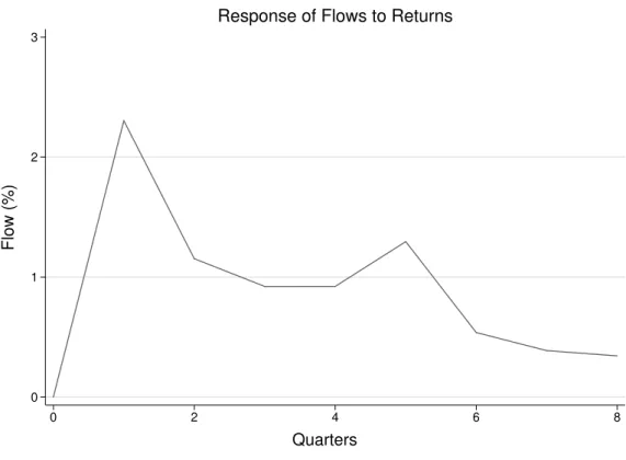
2.3 Response of flows to returns . . . 27
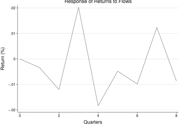
2.4 Response of returns to flows . . . 29
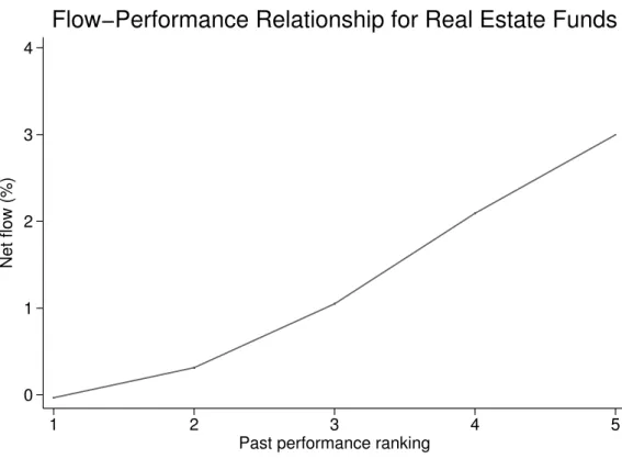
2.5 Flow-performance relationship for real estate funds . . . 32
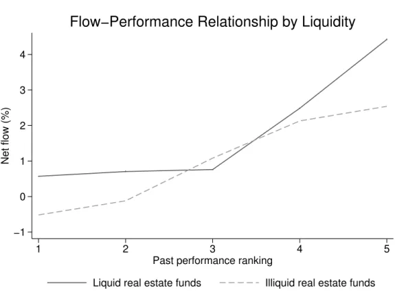
2.6 Flow-performance relationship by liquidity . . . 34
3.1 Fund openings, total AuM and average fund size . . . 55
3.2 Effects of family-objective inflows on fund opening probability . . . 68
3.3 Effects of family size on fund opening probability . . . 70
3.4 Effects of family assets in an investment objective on fund opening probability . . . 71
3.5 Countries with significant open-end real estate fund markets . . . 77
3.6 Average fund size of open-end real estate funds compared to other asset classes . . . 79
4.1 Cumulative (log-) returns of portfolios sorted by NAV spreads . . . 100
List of Tables
2.1 Descriptive statistics for aggregate and fund level variables . . . 20
2.2 Contemporaneous and lagged correlations for aggregate variables . . . 23
2.3 Vector autoregression results for aggregate flows and returns . . . 26
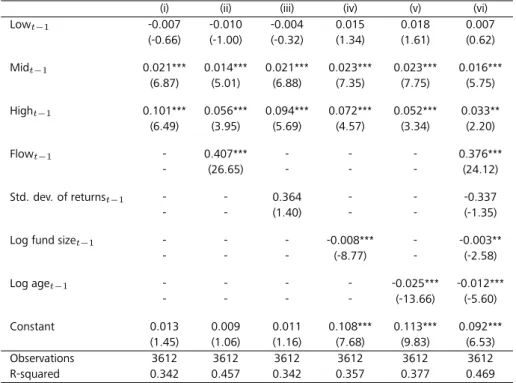
2.4 Effect of relative performance on individual real estate fund flows . . . 33
2.5 Effect of liquidity on the flow-performance relationship . . . 36
2.6 Effect of low liquidity on the flow-performance relationship . . . 39
3.1 Distribution of the sample of fund openings . . . 56
3.2 Distribution of the explanatory variables . . . 61
3.3 Fund openings and fund flows . . . 63
3.4 Determinants of new fund openings . . . 67
4.1 Descriptive statistics of returns and NAV spreads . . . 94
4.2 Correlations of country-level returns and NAV spreads . . . 96
4.3 Performance and characteristics of portfolios sorted by NAV spreads . . 98
4.4 Risk-adjusted performance of portfolios sorted by NAV spreads (CAPM) 102 4.5 Risk-adjusted performance of portfolios sorted by NAV spreads (Fama- French three-factor model) . . . 103
V
Introduction
The question ofwhetherto invest in real estate is easily answered by numerous asset allocation studies that have found real estate should play a significant role in optimal multi-asset portfolios.1 The benefits of real estate as an asset class are often attributed to a favorable risk-return profile due to relatively stable rental income and a low corre- lation with other asset classes such as stocks and bonds. Furthermore, as a real asset, it is typically assumed to possess significant inflation-hedging capabilities. There are, however, challenges that need to be addressed when a real estate investment is con- sidered. First of all, a direct investment in physical real estate is inherently illiquid as transaction costs are high and transaction periods can be substantial. Second, the private real estate market is rather opaque, due to the heterogeneity of each property and the lack of a central marketplace. Thus, information costs tend to be high. Third, the indivisibility of direct property results in high minimum investment requirements, which is a challenge to the construction of well-diversified property portfolios.
As a result, direct property investments are often an option only for large institu- tional investors with 1) long investment horizons that can attenuate illiquidity issues, 2) the necessary expertise to solve information problems, and 3) sufficient capital to facilitate the construction of well-diversified portfolios. For all other investors, the question ofhowto gain exposure to real estate as an asset class is a non-trivial one.
1See Seiler et al. (1999) for a review of the early academic literature on optimal allocations to real estate. Suggested allocations typically range from 15% to 20%. More recent research by MacKinnon and Al Zaman (2009) considers the effect of the investment horizon. The authors find that, for medium- to long-term investors, optimal allocations to real estate can increase to as high as 23%-31% due to the decreasing correlation of real estate with stocks and bonds.
Introduction
The hurdles in obtaining the desirable risk-return characteristics of real estate pro- vide a rationale for the existence of real estate investment vehicles as a form of finan- cial intermediation. However, it is important to keep in mind that although financial intermediation can reduce the problems of direct real estate investments, the prob- lems themselves do not cease to exist (Sebastian, 2003). This dissertation is concerned with the tensions that can arise when an inherently illiquid asset such as direct real estate is transformed into an investment vehicle that is traded on a day-to-day basis.
In general, real estate investment vehicles can be classified into open-end and closed-end funds. The key difference (which is central to this dissertation) is the way liquidity is provided. In the case of open-end funds, liquidity is created by the fund (or the sponsor of the fund), which regularly sells new shares and redeems existing shares. Importantly, it is the fund that calculates the price per unit, which depends primarily on regularly appraised property values and is hence tightly linked to the value of the underlying assets. In contrast, the paid-in capital of closed-end funds is con- stant. Once the initial capital is collected, the fund is closed, and the shares trade on public exchanges where the price results from supply and demand, and is not always on par with the value of the underlying assets.
In summary, open-end funds create liquidity through a variable number of shares at afixed price(at least in the short term), whereas closed-end funds create liquidity through avariable share price, whereby thenumber of shares is fixed. In both cases, the investment vehicle ends up being more liquid than the underlying asset, which may lead to the following tensions between the liquidity of the fund and the liquidity of the underlying assets.
Open-end funds respond to the time-varying demand of investors for the vehicle by adjusting the number of shares. Tensions may arise when investors attempt to redeem shares at a faster rate than the fund is able to liquidate its underlying as- sets. To mitigate this problem, open-end real estate funds tend to hold high cash reserves. However, the cash reserves are limited and ultimately, open-end funds may have to suspend share redemptions until enough properties are sold to pay the exiting investors. In this event, the funds will temporarily cease to provide liquidity transfor- mation.
2
In the case of closed-end funds, the time-varying demand of investors for the ve- hicle is matched through a variable share price on public exchanges. Here, tension may arise when the price for the investment vehicle changes at a faster rate faster rate than justified by changes in the value of the underlying assets. Ultimately, price and fundamental value may deviate from each other to an extent that the return dy- namics no longer justify the high optimal allocation to real estate found in numerous multi-asset portfolio studies. In summary, the liquidity-providing mechanism is also the Achilles heel of both types of investment vehicles.
This dissertation examines three key issues related to the tension between asset and fund liquidity of real estate investment vehicles. The first part addresses real estate fund flows, which are at the core of the liquidity-providing mechanism of open-end real estate funds. When the number of newly issued shares exceeds the number of redeemed shares, a positive fund flow is measured. In contrast, when more investors exit their investments, open-end funds experience outflows, and the fund’s cash re- serves are reduced. When the cash reserves of the fund are low, or if the outflows are particularly high, the fund is at risk of becoming illiquid. To rebuild cash reserves (or to reopen the fund if it has temporarily suspended share redemptions), the fund may be forced to sell properties, which is time-consuming and involves high transaction costs.
Hence, understanding what drives real estate fund flows is of central importance in the case of open-end real estate funds. The general mutual fund literature finds that fund flows into equity mutual funds, where underlying asset illiquidity is not a concern, depend predominantly on a fund’s past performance. As investors tend to disproportionately chase the best past performers, while poorly performing funds are merely sold, the flow-performance relationship is found to be convex (Sirri and Tufano, 1998).
Using a piecewise linear regression framework, this dissertation confirms the con- vexity of the flow-performance relationship for a sample of 25 German open-end real estate funds over the September 1990 to December 2010 period. However, the shape is also found to vary with fund-level liquidity (i.e., cash reserves relative to fund size). Investors are more sensitive to poor past performance when fund liquidity is low. Also, the best-performing funds tend to be chased less as their risk of becoming
Introduction
illiquid increases. Overall, the results suggest that open-end real estate fund investors are aware of the risk associated with low fund-level liquidity.
The second part of this dissertation examines the determinants of fund openings, particularly whether the decision to open a new open-end real estate fund is different from other asset classes such as stocks or bonds, where there is no discrepancy be- tween asset and fund liquidity. The decision to launch a new mutual fund is essentially a cost-benefit trade-off. This dissertation finds that this trade-off generally tends to favor fund openings in liquid asset classes such as stocks or bonds. In the case of real estate, this trade-off is significantly influenced by the liquidity risk of open-end funds.
The dataset used here consists of 2,127 fund openings in 12 investment objectives for 76 fund families within the German mutual fund industry over the 1992-2010 period. A substantial cannibalization effect across the existing real estate funds of a family following a fund opening is documented. Due to the illiquid nature of the underlying assets, this cannibalization effect is a threat for the existing real estate funds of a family. An analysis of the determinants of fund openings using probit regression techniques reveals high inflows into the existing real estate funds of a family are the key to overcoming the cannibalization barrier. This factor is far less important for fund openings in other asset classes, where liquidity issues do not play a role.
Additional findings reveal that, in contrast to other asset classes, real estate fund openings are not sensitive to proxies for economies of scale or scope at a fund family level. This finding is consistent with strong fund-level economies of scale that provide an incentive to allow existing real estate funds to grow large. Overall, the results suggest that the determinants of real estate fund openings cannot be subsumed under a general fund opening framework because of differences in specific features of the underlying assets.
The third part of this dissertation is related to the tension between asset and fund liquidity of closed-end real estate funds. Publicly traded real estate stocks are the most prominent representative of closed-end real estate funds in many countries. Because they are traded daily on public exchanges, the liquidity of the investment vehicle is often higher than the liquidity of the underlying assets, and hence stock prices may change more rapidly than justified by changes in the values of the underlying prop-
4
erties. In other words, the prices of publicly traded real estate stocks may be too variable relative to value changes of the underlying assets. To investigate whether price and fundamental values have deviated too far, this dissertation tests whether an investment strategy that is long in real estate stocks with the most attractive ratios of price-to-fundamental value can produce significant excess returns.
The true fundamental value of real estate funds is unobservable. However, the net asset value (NAV) of publicly traded real estate stocks in fair value-based accounting regimes provides a relatively robust approximation. This is especially true when com- pared to the common book value of equity for general stocks that is used as a proxy for fundamental value in many asset pricing studies. Therefore, the analysis in the third part of this dissertation is based on a sample of 255 listed property holding com- panies in 11 countries with fair value based-accounting regimes over the 2005-2014 period. The key variable of interest is the ratio of price-to-NAV, or the NAV spread, which measures discrepancies between price and value. The results provide strong evidence in favor of the theory that market prices of real estate stocks can deviate too far from fundamental values. Investing in a global portfolio of the most under- priced real estate stocks relative to the average ratio of price to fundamental value in a country provides annualized excess returns of 8.0%. Even after controlling for common risk factors, risk-adjusted returns remain statistically significant. The implica- tion is that stock price variability on public exchanges does not always reflect changes in fundamental values. Hence, the liquidity transformation of closed-end real estate funds may result in a loss of the risk-return characteristics of the underlying assets.
Chapter 2
Real Estate Fund Flows and the Flow-Performance Relationship
This paper is the result of a joint project withDavid H. Downs,Steffen Sebastian, and Christian Weistroffer.
Abstract
This paper examines the flow-performance relationship for direct real estate invest- ment funds. Combining a unique data set with a VAR model framework, we find evidence that investors chase past returns at the aggregate level. However, we find against a market timing hypothesis - real estate fund flows do not seem to predict sub- sequent returns. Additional findings indicate aggregate flows into direct real estate funds are serially correlated and negatively related to changes in the risk free rate. Our analysis of individual fund flows is motivated by a growing body of literature that ad- dresses the flow-performance relationship and the effect of illiquid assets. Overall, we find the flow-performance relationship for direct real estate investment funds is con- vex. This finding is consistent with studies based on funds with more liquid underlying assets such as equity funds. More importantly, we find that the flow-performance shape varies with fund-level liquidity. Individual fund flows are less sensitive to poor performance as liquidity increases. The flow-performance sensitivity is higher for high performing funds as liquidity increases. Together these results imply that fund liquidity
6
increases the flow-performance convexity of real estate funds. The implications are that investors are more sensitive to fund-level underperformance (i.e., more likely to sell), when there is increased liquidity risk.
Real Estate Fund Flows and the Flow-Performance Relationship
2.1 Introduction
The mutual fund literature provides clear evidence that investors buy those funds with the highest past returns (Ippolito, 1992; Sirri and Tufano, 1998; Guercio and Tkac, 2002). The literature also reports that investors do not withdraw money from the worst performing funds to the same degree. Consequently, the relationship between fund flows and performance of individual funds is described as convex. Most studies on the relationship between fund flows and performance are limited to funds which invest in liquid asset classes such as stocks and bonds. As a result of the underlying asset liquidity, these funds are generally considered liquid funds. Chen et al. (2010) analyze the flow-performance relationship while differentiating among the liquidity of stocks held by mutual funds. They document that funds investing in less liquid stocks exhibit a stronger sensitivity of outflows to poor past performance than funds with liquid assets. They argue an investor’s tendency to withdraw increases when there is a concern for the damaging effect of other investor’s redemptions. This rationale follows as outflows in illiquid funds result in more damage to future performance due to higher trading costs. The results of Chen et al. (2010) suggest that the degree of liquidity of the underlying asset may have an effect on investor behavior. This raises the question how fund investors behave if the underlying asset is completely illiquid as in the case of direct real estate investments.
The literature on the flow-performance relationship in the context of real estate is sparse. In this case, data limitations restrict the scope of research questions addressed.
Fisher et al. (2009) and Ling et al. (2009) derive capital flows of institutional investors from their transactions in the US and UK property markets in order to analyze whether the transactions of these investors cause price pressure at the aggregate level. This is problematic as each transaction also has a counterparty. Thus it remains unclear why the transactions of one sub-segment of investors (here, institutional investors) would cause price pressure while those of the other sub-segment of investors would have to cause the opposite. These authors also analyze whether investors chase past returns.
In that context, their measure of flows and returns has another challenge. Flow data that are derived from transactions do not precisely reflect the point of time when the decision to invest in real estate has actually been made. The time lag until property
8
transactions are finally closed is often a substantial and time-varying. Thus, their flow measure might be attributed to performance chasing behavior (or not), although market conditions may have been completely different when the actual investment decision took place.
Another strand of real estate studies on the flow-performance relationship is based on REIT mutual funds. Ling and Naranjo (2006) analyze the relationship between ag- gregate flows into REIT mutual funds and aggregate REIT returns. Chou and Hardin (2013) study the flow-performance relationship at the level of individual REIT mutual funds. However, the REITs held by REIT mutual funds are publicly traded, liquid se- curities. Thus, investments into REIT mutual funds may not be affected by illiquidity considerations that play a role in the context of direct real estate investments. Fur- thermore, flows into REIT mutual funds may only have an effect on REIT prices. As fund flows do not cause transactions in the direct property market the effect on the underlying asset seems only remotely possible. Finally, Ling and Naranjo (2003) ex- amine total capital flows into REITs (i.e. equity issuances and net debt changes), but their flow data is based on financing decisions of the REIT management and hence not suited to analyze investor behavior in the tradition of the mutual fund literature.
The aim of this study is to address these limitations by investigating the flow- performance relationship of direct real estate investment funds. Our analysis is based on a dataset of German mutual funds over the September 1990 to December 2010 period. Germany is one of the few places worldwide where investors have the oppor- tunity to invest in direct real estate investment funds with an open-ended structure.
Unlike REIT mutual funds, which invest in liquid, publicly traded REITs, German open- end real estate funds invest directly in real property. In order to be able to absorb negative cash flow shocks without immediately having to engage in costly transac- tions, real estate funds hold high cash reserves which serve as a liquidity insurance.
Up to 50% of their assets under management (AuM) are invested in cash, which is substantially higher than the 4-5% typically reported for equity mutual funds. When the liquidity ratio falls below 5%, the fund is legally required to stop the redemption of shares until liquidity is restored.
This setting provides several advantages to study investor behavior when the un- derlying asset is particularly illiquid. First, our flow data is a high-quality, contempora-
Real Estate Fund Flows and the Flow-Performance Relationship
neous measure of fund investor decisions to invest in real estate. Thus, we measure precisely how investors react to performance and do not have to rely on transaction data which are a lagged measure of real estate investment decisions. Compared to flows into REIT mutual funds, our flow data enables us to analyze the link between the direct property market and public security markets as the returns of real estate funds are based on appraisals and property transactions, and not on public security returns.
Furthermore flows into real estate funds are ultimately invested into (or divested from) the direct property market, while REIT mutual fund flows merely affect REIT prices.
Our initial analysis focuses on the flow-performance relationship at the aggregate level. Here, we follow the methodological approach of Fisher et al. (2009), Ling et al.
(2009) and Sebastian and Weistroffer (2010), and use Vector Autoregression (VAR) analysis to capture the dynamic relationship between flows and returns, while con- trolling for exogenous factors that may affect investor behavior. We empirically test whether investors chase past returns at the aggregate level. We find aggregate flows into real estate funds are positively related to prior fund returns which is consistent with return chasing behavior of real estate fund investors. This results stands in con- trast to the findings of Warther (1995) who finds no evidence of return chasing of behavior of equity fund investors at the aggregate level.
We also examine whether aggregate flows have an effect on subsequent returns.
As we do not observe flows and returns in sub-markets by property type but only flows and returns of the fund as a whole, we cannot test the price pressure hypothesis.
Instead, our data set enables us to examine whether investors possess market timing ability on an aggregate level in the context of real estate funds. More specifically, we test whether investors move into real estate funds prior to future outperformance, and out of real estate funds before they underperform. However, we find no evidence supporting the market timing hypothesis for real estate funds on an aggregate basis.
Additional analysis shows that aggregate flows and returns are serially correlated.
Aggregate flows are negatively related to lagged changes in the risk free rate, which is consistent with investors viewing real estate funds as a low risk investment substitute for cash. Furthermore, we find aggregate real estate returns are positively related to the level of the risk free rate in the previous period. The analysis is complemented by
10
impulse response functions in which we examine this dynamic relation over a longer horizon.
Next, we examine the flow-performance relationship for individual real estate funds.
This analysis enables us to determine whether the return-chasing behavior of investors observed at the aggregate level is also evident as investors choose among different funds. In addition, we address the question whether the flow-performance relation- ship is affected by fund liquidity. We follow the approach of Sirri and Tufano (1998) and model investor choice between real estate funds using a piecewise linear ap- proach with fund- and time fixed effects. We find that investors respond to past performance when selecting individual funds. The flow-performance relationship for real estate funds is convex. Top-performing funds receive disproportionally large in- flows in the following period. While the underlying assets of real estate funds are illiquid, we find no evidence that investors punish poor performance. This result con- tradicts the prediction of Chen et al. (2010) that funds with less liquid assets show a stronger response of flows to poor performance.
In additional analysis we model the effect of fund liquidity on the flow-performance relationship by interacting past performance with the liquidity ratio of the fund. We find that fund liquidity affects the shape of the flow-performance relationship. Fund liquidity increases the flow-performance sensitivity for strong performing funds while it decreases the sensitivity for poorly performing funds.1 This result suggests investors chase past performance less and flee poor performance more aggressively when the fund liquidity is a constraint. Our findings contribute to the literature by highlight- ing direct real estate investment funds and the role of fund liquidity for the flow- performance relationship.
The remainder of this paper is organized as follows. Section 2.2 introduces the related literature and our hypotheses. The dataset and descriptive statistics are intro- duced in Section 2.3. Section 2.4 contains our research methodology and the empiri- cal results for the aggregate analysis. Section 2.5 provides the research methodology and results for the fund level analysis. Section 2.6 provides our conclusions.
1Sebastian and Weistroffer (2010) examine the flow-performance relationship for 18 German real estate funds from 1990-2008. However, they do not control for liquidity. In contrast to our results, they find a linear relationship between flows and returns.
Real Estate Fund Flows and the Flow-Performance Relationship
2.2 Related Literature and Hypotheses
2.2.1 Performance Chasing
Chasing past performance can be rational if past performance contains information about future performance. In the public stock markets, past performance is generally not a good indicator of future performance. Hence, it is not surprising that Warther (1995) finds no evidence that aggregate fund flows into equity mutual funds are pos- itively related to past returns. The REIT literature provides some evidence that the returns of REITs are more predictable than those of common stocks (e.g. Nelling and Gyourko (1998) or Ling et al. (2000)). Thus, the finding of Ling and Naranjo (2006) that aggregate flows into REIT mutual funds are positively related to prior aggregate REIT returns could be interpreted as a case of rational investor behavior. Return chas- ing might be even more of an issue in the private real estate markets, where the autocorrelation of direct real estate returns is well documented. However, theextant literature provides mixed evidence regarding whether or not investors chase past per- formance in the private real estate market. While Ling et al. (2009) find support for return chasing behavior of institutional investors UK data, Fisher et al. (2009) come to the opposite conclusion with institutional transaction data from the US.
Our data of direct real estate investment funds provides a unique setting to study whether or not real estate investors chase past returns. As the returns of real estate funds are predominantly based on appraisal values and rental income, they should show patterns similar to those documented for return indices of private real estate markets. Consequently, at least in the short term, investors of real estate funds may successfully predict future performance from past fund returns and invest their money accordingly. Thus, we formulate our hypothesis of return chasing behavior at the aggregate level as follows:
Hypothesis 1: Investors chase past performance (i.e., aggregate net flows into real estate funds are positively related to prior performance).
12
2.2.2 Market Timing
If investors simultaneously invest in or withdraw money from several mutual funds within the same investment category, the returns of the underlying assets may be affected. Warther (1995) finds evidence of price pressure through aggregate mutual fund flows. He reports that aggregate flows into equity mutual funds are positively related to contemporaneous stock returns, while he finds no relationship between returns and lagged flows. Coval and Stafford (2007) find evidence of price pressure across a common set of securities held by distressed funds. Funds experiencing large outflows tend to decrease existing positions, while funds experiencing large inflows tend to expand existing positions. Using aggregate flows into REIT mutual funds, Ling and Naranjo (2006) also only document a contemporaneous relationship between REIT returns and aggregate REIT mutual fund flows, but they do not find that flows predict returns. In the private real estate market, Fisher et al. (2009) find that US- based capital flows predict subsequent returns, whereas Ling et al. (2009) find no support for the price pressure hypothesis in the UK.
In contrast to prior studies, our data set enables us to examine whether investors possess market timing ability on an aggregate level. Unlike the prior work, we do not claim to test the price pressure hypothesis as our measure of returns is based on the aggregate performance of the real estate funds in the sample as opposed to underlying asset prices. More specifically, we test whether investors move into real estate funds prior to future outperformance, and out of real estate funds before they underperform. Bhargava et al. (1998) identify a short-term trading strategy for open-end mutual funds where investors can exploit international correlations of stock markets by buying mutual funds whose NAVs do not yet reflect information released during the US trading day. A similar, yet longer-term investment strategy might be profitable for real estate funds. The returns of real estate funds are predominantly based on annual appraisals which are periodically updated for the whole portfolio of the fund. Investors might trade on anticipated swings in the real estate market before they are reflected in the new appraisals and hence in the net asset values (NAVs) of the funds. For example, investors might foresee a significant revaluation of fund assets in the near future. This leads us to our market timing hypothesis:
Real Estate Fund Flows and the Flow-Performance Relationship
Hypothesis 2a: Aggregate flows into real estate funds predict future perfor- mance (i.e., investors of real estate funds exploit anticipated return swings).2,3
However, even if inflows and outflows occur due to rational expectations about future performance, the fund flows themselves may have a negative impact on fund performance. In the short term, high inflows increase a fund’s share of lower yielding cash holdings. Therefore, potentially successful market timing may be masked by the dilution effect of fund flows on returns. Greene and Hodges (2002) find that daily fund flows into equity mutual funds have a dilution effect of annualized 0.48%. This effect may be even stronger for real estate funds, because the high liquidity ratios persist until additional property acquisitions are completed, which takes substantially longer compared to equity funds. Furthermore, it is well known from other asset classes such as equity mutual funds (Chen et al., 2004), private equity funds (Lopez-de Silanes et al., 2013), and hedge funds (Fung et al., 2008), that capacity constraints are associated with the lower returns of larger funds. In the medium to longer term, higher liquidity ratios will ultimately transmit into property transactions. This may force the fund management to engage in less profitable property transactions, providing another reason why fund flows might have a negative impact on subsequent returns. The two contradicting effects are reflected in our alternative hypothesis about the relationship between fund flows and subsequent performance:
Hypothesis 2b: Aggregate flows into real estate funds dilute fund performance due to capacity constraints and by increasing a fund’s share of lower yielding cash holdings.
2.2.3 Flow-Performance Convexity
There are numerous studies in the mutual fund literature that find a strong relation- ship between past performance and subsequent flows into individual mutual fund
2We acknowledge the 5% front-end load fee for real estate funds is a hurdle that makes market timing less profitable for investors that buy into the market. However, as each investor has to pay this fee, it is still better to buy into the market when it is perceived to be relatively cheap than in fairly-priced or overvalued periods. In contrast, there is no redemption fee when investors redeem shares, thus, there are no barriers to exiting an expensive market.
3In July 2013, a new law came into force which introduced a minimum holding period of 24 months as well as a notice period of 12 months. These regulatory changes can be seen as further hurdles for market timing, though they became effective after the end of our sample period.
14
flows (Ippolito, 1992; Sirri and Tufano, 1998; Guercio and Tkac, 2002). Most of these studies find that investors tend to respond more positively to good performance rel- ative to poor performance, i.e. winners are bought more intensely than losers are sold. This phenomenon results in a convex shape of the flow-performance relation- ship. The shape of the flow-performance relationship can have important implications for various market participants. For example, Chevalier and Ellison (1997) argue that fund managers are encouraged to take more risk if outperformance is associated with significant inflows while investor reaction to poor performance is more muted. The flow-performance relationship may also have an effect on the performance persis- tence of mutual funds. Chen et al. (2004) find that fund size is negatively related with fund performance. The flow-performance relationship determines to what ex- tent large funds will be affected by these diseconomies of scale, as it determines to what extent past performance results in excessive inflows (Berk and Green, 2004).
More recent research by Chen et al. (2010) finds the flow-performance relationship depends on a mutual fund’s underlying asset liquidity. The authors document that funds investing in less liquid stocks exhibit a stronger sensitivity of outflows to bad past performance than funds with liquid assets. The hypothesized rationale behind this is that investors fear the damaging effect of other investor’s redemptions which lead to further underperformance due to high transaction costs which are caused by the outflows – a problem that is likely to apply to real estate funds, as well.
The illiquidity of direct real estate is manifest in high property transaction costs and long transaction periods. In the short term, high cash reserves protect real estate funds from costly fire sales, when a large amount of investors redeem their shares.
Still and at least in the medium term, real estate funds have to react to outflows by selling properties if they want to maintain their target liquidity ratios. As in the case of mutual funds that hold illiquid stocks, these transactions may have adverse effects on fund performance. Compared to equity mutual funds that invest in liquid stocks, the financial fragility that is caused by illiquid underlying asses is not an issue as long as investors have no reason to redeem their shares. This situation may change if in- vestors anticipate that other investors will redeem their shares which would result in costly underperformance. Chen et al. (2010) argue that fundamental events may have an amplifying effect if they increase an investor’s incentive to take action in the
Real Estate Fund Flows and the Flow-Performance Relationship
expectation that other investors will take the same action. A real estate fund’s un- derperformance relative to its peers might be such a coordinating event that triggers substantial outflows as a result of the anticipation of other investor redemptions. This scenario is the basis of our third hypothesis, that real estate fund flows are sensitive to poor performance and hence, the flow-performance relationship is not convex, but linear.
Hypothesis 3: The flow-performance relationship for real estate funds is linear (i.e. fund flows are sensitive to both, strong and poor performance).
2.2.4 Fund Liquidity
Hypothesis 3 addresses the role of the illiquidity of the underlying assets, not the liquidity of the fund itself. The liquidity of the fund may however have a direct impact on fund flows and hence the flow-performance relationship.
A real estate fund is either liquid or not. Investors may redeem their shares directly to the fund family at NAV, which is calculated on a daily basis. If, however, the liquidity ratio of the fund falls below 5%, real estate funds are legally obligated to stop the redemption of shares. In this event, the fund is “closed” for a period of up to 24 months. During this time, the fund tries to build sufficient cash reserves either by selling properties or by attracting new inflows. If the fund fails to build sufficient cash reserves, it may close for a second time. After three unsuccessful re-openings, the fund finally has to be liquidated and pay out the proceeds to the investors. Until the fund reopens, investors have no access to their money, unless they decide to sell their shares on a secondary market often for a substantial discount to NAV.
From the investor’s point of view, the temporary closing of a real estate fund im- plies that the fund becomes illiquid from one day to another. It is the fund’s liquidity ratio that determines the likelihood of this unpleasant scenario. High liquidity ratios provide insurance for the fund and its investors. In contrast, low liquidity ratios in- crease the probability of fund illiquidity and may incentivize investors to redeem their shares before it is too late. We argue that the flow-performance relationship for real estate funds is conditional on the liquidity of the fund. Investors base their investment decision on past performance as long as the fund is liquid. However the risk of illiq-
16
uidity may dominate other factors when the funds’ liquidity ratio is low. Hence, the impact of past performance should be less pronounced in such circumstances. We formulate our hypothesis of fund liquidity as follows:
Hypothesis 4: The flow-performance relationship for real estate funds is condi- tional on the liquidity of the fund (i.e. only liquid real estate funds are sensitive to past performance).
2.3 Data and Descriptive Statistics
2.3.1 Data Sources, Sample Description and Definitions
Our empirical study is based on a survivorship bias-free sample of German open-end real estate funds for the September 1990 to December 2010 period. We obtain monthly information about absolute net flows, i.e., actual purchases minus redemp- tions,4 and the size of the funds (i.e., AuM) from the German Investment and As- set Management Association (BVI). The BVI Investment Statistics report is the core overview of portfolios and inflows in the German investment industry. The BVI col- lects information about net flows and AuM directly from its members which represent approximately 99 percent of the German mutual fund industry AuM. Monthly fund returns are obtained from Morningstar and Datastream. The risk free rate (Germany 3-month treasury bill rate) and the three Fama-French risk factors for Germany are from Stefano Marmi’s web site.5
The final sample is comprised of 25 German open-end real estate funds. We ex- clude semi-institutional funds from the sample as they are primarily intended for in- stitutional investors.6 At the beginning of our sample period in September 1990, we
4Our measure of fund flows is based on actual buying and selling decisions of investors, whereas most studies covering the US or UK market approximate net flows by the following formula: Flow(t)=(Fund size(t)-Fund size(t-1)*(1+Fund return(t)))/Fund size(t-1). This approximation formula assumes that all flows occur at the end of the period. Furthermore, dividend payments are treated as outflows, although they do not reflect investor decisions. In contrast, our flow data treats dividend reinvestments as an inflow as investors might be more willing to reinvest their dividends into the fund if they are satisfied with the performance.
5http://homepage.sns.it/marmi/DataLibrary.html.
6Legally, semi-institutional funds are retail funds. The similarity stops there. The minimum investment for semi-institutional funds starts at half a million Euros. We identify 13 semi-institutional fund openings in our sample.
Real Estate Fund Flows and the Flow-Performance Relationship
observe 10 real estate funds. Fifteen real estate funds were opened over the sample period. Two funds were discontinued, with fund volume partly shifting to other funds.
By the end of 2010, 24 funds existed in total. Twelve of these funds were “frozen”
or “in liquidation” as they were hit by the global financial crisis. A frozen fund no longer redeems shares, but it continues to sell new shares. As a result, their net flows are either positive or zero. Our analysis addresses the behavior of all fund investors, i.e., we are also interested in the factors that cause investors to redeem their shares and this is no longer possible when a fund is frozen. Consequently, only observations for non-frozen funds are used in the sample, though we include the outflows for the month in which the fund moves to a frozen status. When a fund reopens, we typi- cally observe high outflows as investors regain the opportunity to redeem their shares.
Therefore we wait for one month after the reopening for a fund to return to the sam- ple. In additional analysis, we also use data on the liquidity ratios of the funds. We hand-collect data on the cash holdings of the real estate funds from their annual and semi-annual reports.
We analyze the flow-performance relationship at, both, the aggregate level and the level of individual real estate funds. Our key variable of interest is the percentage net flow, or the growth rate of new money, which is defined as the absolute net flow, normalized by the size of the fund at the end of the previous period:
F lowi,t = AbsoluteN etF lowi,t F undSizei,t−1
(2.1) At the aggregate level we are also interested in the effect of flows on returns. Here, we follow the literature and use quarterly data. This seems plausible given that returns are affected by a time lag until flows transmit into property transactions. Thus, we use the total net flows into all real estate funds over the quarter relative to the total size of all real estate funds at the end of the previous quarter. Aggregate returns are defined as the value-weighted return of all real estate funds over the quarter.
At the fund level, we focus on fund flows. Thus, we conduct the fund level analysis with monthly data in order to make use of the highest data frequency available. The liquidity ratio of a fund is a key explanatory variable used in the fund-level analysis.
The liquidity ratio is defined as the total fund holdings of liquid securities (cash and 18
short-term investments) relative to the size of the fund:
Liquidityi,t = CashReservesi,t
F undSizei,t
(2.2) Note that real estate funds also use leverage of up to 50% of the total assets. Thus, the liquidity ratio refers to the equity portion or NAV of the fund and does not reflect the share of total assets invested cash. For example, all else being equal, a liquidity ratio of 20% implies that the fund is able to redeem 15% of all outstanding shares before the critical liquidity ratio of 5% is reached. As we only observe half-yearly updates of a fund’s cash holdings, the liquidity ratio only changes every six months.
To ensure our results at the level of individual real estate funds are not driven by outliers, we winsorize flows at the bottom and top 1% of the distribution. At the aggregate level, there is no need to winsorize, as the potential effect of outliers disappears by aggregating the data.
2.3.2 Descriptive Statistics
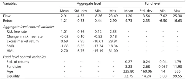
Table 2.1 presents the descriptive statistics for flows and returns at the aggregate level and at the level of individual funds over the 1990:3 to 2010:4 period. Furthermore, Table 2.1 contains the descriptive statistics of the employed control variables. The first four columns show the mean, standard deviation, minimum, and maximum for the quarterly aggregate level variables. The next four columns show the same metrics for the monthly fund level variables. Note that fund level returns and their standard deviations refer to monthly measures of the total return over the previous twelve months, while all other variables refer to monthly data.
We first focus on the aggregate level statistics in the first four columns of Table 2.1.
On average, real estate funds experienced positive growth rates of 2.91% per quarter, in excess of the growth in AuM that is caused by positive returns. The standard devi- ation associated with these growth rates is 4.63%. The minimum net flow reveals a maximum loss of 8.26% of AuM in a single quarter, while the maximum value equates to a quarterly inflow of 23.49%. Over the same period, the average value-weighted quarterly return of all real estate funds is 1.21%, which equates to an annualized total
Real Estate Fund Flows and the Flow-Performance Relationship
Table 2.1: Descriptive statistics for aggregate and fund level variables
Variables Aggregate level Fund level
Mean Std. dev. Min. Max. Mean Std. dev. Min. Max.
Flow 2.91 4.63 -8.26 23.49 1.20 3.54 -7.02 25.30
Return 1.21 0.53 0.44 2.90 4.73 2.35 -6.50 16.63
Aggregate level control variables
Risk free rate 1.01 0.56 0.12 2.33 - - - -
Change in risk free rate -0.02 0.10 -0.53 0.18 - - - -
Excess market return 0.69 7.95 -18.61 29.91 - - - -
SMB -1.88 6.35 -17.24 18.34 - - - -
HML 2.70 6.75 -15.19 31.00 - - - -
Fund level control variables
Std. of returns - - - - 0.27 0.24 0.04 1.79
Fund size - - - - 3.23 2.68 0.037 11.90
Age - - - - 225.80 160.06 14 556
Liquidity - - - - 32.75 14.24 5.00 99.55
This table contains the descriptive statistics for the aggregate and fund level variables used throughout the analysis over the September 1990 to December 2010 period. Aggregate level flow (%) = total absolute net flow of the quarter into all real estate funds divided by the total size of all real estate funds at the end of the previous quarter; Fund level flow (%) = absolute net flow of the month into the fund divided by fund size at the end of the previous month; Aggregate level return (%) = value-weighted return of the quarter of all real estate funds; Fund level return (%) = fund return of the past 12 months; Risk free rate = Germany 3-month treasury bill rate in EUR; Change in risk free rate (%) = change in the Germany 3-month treasury bill rate in EUR; Excess market return (%) = Germany stock market return in excess of the risk free rate in EUR; SMB (%) = Germany small-firm minus big firm return factor in EUR; HML (%) = Germany high book-to-market minus low book-to-market return factor in EUR; Std. of returns (%) = fund return volatility of the past 12 months; Fund size (billions of EUR) = fund size at the end of the month; Age = fund age in months; Liquidity (%) = cash holdings of the fund divided by fund size.
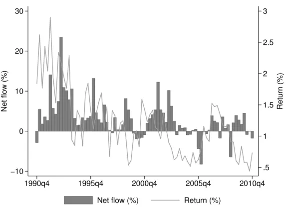
return of 4.84%. Thus, the average return of real estate funds in excess of the risk free rate is 0.8% per year and, thus, substantially lower than the annualized excess re- turn of the German stock market (2.76%). The standard deviation of quarterly returns of 0.53% indicates real estate funds are a low risk investment. The risk-return profile that should appeal to more risk-averse investors is complemented by a minimum quar- terly return that is still positive (0.44%). In Figure 2.1, we plot aggregate flows and returns over the sample period. Flows are measured on the left vertical axis, returns are measured on the right vertical axis. Consistent with the correlation coefficients, the co-movement indicates that investors tend to invest more during times of high returns and less during periods of low returns.
Next, we turn to the descriptive statistics at the individual fund level. As expected, the fund level numbers show a wider distribution compared to the aggregate level.
Even after winsorizing, we observe monthly outflows of up to -7.02% and maximum inflows into individual funds of more than 25% of AuM. The average monthly net flow into individual real estate funds is 1.2%, and thus higher than at the monthly equivalent at the aggregate level. This suggests that smaller funds experience stronger growth relative to large funds.
20
.5 1 1.5 2 2.5 3
Return (%)
−10 0 10 20 30
Net flow (%)
1990q4 1995q4 2000q4 2005q4 2010q4
Net flow (%) Return (%)
Figure 2.1: This figure shows the time series of aggregate fund flows and returns of all real estate funds between September 1990 and December 2010.
At the disaggregated level, real estate funds also appear slightly more risky. The average 12-month return of the real estate funds in our sample (measured at a quar- terly frequency) is 4.73% with a standard deviation of 2.35% and extreme values of -6.50% and 16.63%. The average real estate fund has a size of 3.23 billion Euros. The standard deviation of fund size is 2.68 billion Euros. The largest fund in our sample has a size of 11.90 billion Euros, which compares to a minimum fund size of only 37 million Euros.
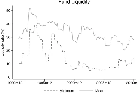
We observe substantial heterogeneity in the liquidity ratios of the funds in our sam- ple. The average liquidity ratio is 32.75% with a standard deviation of 14.24%. The lowest liquidity ratio is 5.00% and therefore just above the critical value of 5%. The maximum liquidity ratio is 99.55%. Liquidity ratios near 100% may occur for young funds which have already raised money, but not yet closed any property transactions, so their assets only consist of cash holdings. Figure 2.2 graphs the mean and mini- mum liquidity ratio for the funds in our sample over the September 1990 to December 2010 period.
Real Estate Fund Flows and the Flow-Performance Relationship
0 10 20 30 40 50
Liquidity ratio (%)
1990m12 1995m12 2000m12 2005m12 2010m12
Minimum Mean
Fund Liquidity
Figure 2.2: This figure shows the mean and minimum liquidity ratios between September 1990 and December 2010.
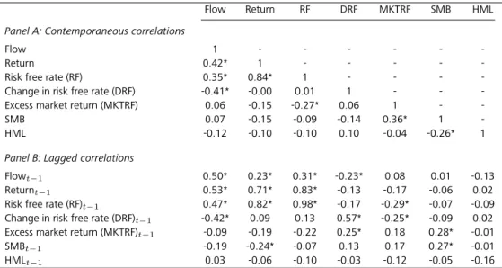
Panel A of Table 2.2 contains the contemporaneous correlations for the aggregate variables. A star indicates that the correlation is statistically significant at the 5% level.
The first column in Panel A reveals a positive and statistically significant correlation between aggregate flows and returns (ρ=0.42). The respective correlation coefficient between flows and lagged returns is even stronger (ρ=0.53). This suggests fund flows may follow returns. The second column of Panel B contains the correlation coefficients between returns and lagged flows. Returns are positively correlated with past flows (ρ=0.23), which is consistent with the market timing hypothesis.
The strong and statistically significant correlation between flows and lagged flows (ρ=0.50) in the first column of Panel B and, likewise, the positive correlation between returns and lagged returns (ρ=0.71) in the second column of Panel B indicate that our main variables of interest are autocorrelated and may follow a unit root process.
However, our tests reject the null hypothesis that these time series contain a unit root, so we include these variables without modifications.
22
Table 2.2: Contemporaneous and lagged correlations for aggregate variables
Flow Return RF DRF MKTRF SMB HML
Panel A: Contemporaneous correlations
Flow 1 - - - - - -
Return 0.42* 1 - - - - -
Risk free rate (RF) 0.35* 0.84* 1 - - - -
Change in risk free rate (DRF) -0.41* -0.00 0.01 1 - - -
Excess market return (MKTRF) 0.06 -0.15 -0.27* 0.06 1 - -
SMB 0.07 -0.15 -0.09 -0.14 0.36* 1 -
HML -0.12 -0.10 -0.10 0.10 -0.04 -0.26* 1
Panel B: Lagged correlations
Flowt−1 0.50* 0.23* 0.31* -0.23* 0.08 0.01 -0.13
Returnt−1 0.53* 0.71* 0.83* -0.13 -0.17 -0.06 0.02
Risk free rate (RF)t−1 0.47* 0.82* 0.98* -0.17 -0.29* -0.07 -0.09
Change in risk free rate (DRF)t−1 -0.42* 0.09 0.13 0.57* -0.25* -0.09 0.02 Excess market return (MKTRF)t−1 -0.09 -0.19 -0.22 0.25* 0.18 0.28* -0.01
SMBt−1 -0.19 -0.24* -0.07 0.13 0.17 0.27* -0.01
HMLt−1 0.03 -0.06 -0.10 -0.03 -0.12 -0.05 -0.16
Flow (%) = total absolute net flow of the quarter into all real estate funds divided by the total size of all real estate funds at the end of the previous quarter; Return (%) = value-weighted return of the quarter of all real estate funds;
Risk free rate (RF) (%) = Germany 3-month treasury bill rate in EUR; Change in risk free rate (%) = change in the Germany 3-month treasury bill rate in EUR; Excess market return (%) = Germany stock market return in excess of the risk free rate in EUR; SMB (%) = Germany small-firm minus big firm return factor in EUR; HML (%) = Germany high book-to-market minus low book-to-market return factor in EUR. * denotes significance at the 5% level.
Fund flows are positively correlated with both, the contemporaneous (ρ=0.35) and the lagged level (ρ=0.47) of the risk free rate. This suggest investors tend to buy real estate funds during times of high interest rates. However, this positive relationship may also be driven by the fact that periods of high real estate returns coincide with high levels of the risk free rate (ρ=0.84). In contrast, aggregate flows into real estate funds are negatively correlated with contemporaneous (ρ=-0.41) and lagged (ρ=-0.42) changes in the risk free rate. The correlations between returns and changes of the risk free rates (i.e., contemporaneous as well as lagged), are not statistically significant.
2.4 Aggregate Flows and Returns
2.4.1 Vector Autoregression (VAR) Methodology
In this section, we empirically test whether investors chase past returns (Hypothesis 1) and whether they possess market timing ability (Hypothesis 2a) or whether aggregate flows have a performance diluting effect (Hypothesis 2b). We employ VAR methodol- ogy to examine the dynamic relationship between aggregate flows and returns of real estate funds. A VAR model is a system of simultaneous equations where the depen-
Real Estate Fund Flows and the Flow-Performance Relationship
dent variables are expressed as linear functions of their own and each other’s lagged values and exogenous variables. Several specifications of the following VAR model are estimated:
F lowt=α1+ XT
i=1
βiF lowt−i+ XT
i=1
γiReturnt−i+X
ωsControls,t−1+ε1,t (2.3)
Returnt=α2+ XT
i=1
βiF lowt−i+ XT
i=1
γiReturnt−i+X
ωsControls,t−1+ε2,t (2.4)
F lowt is the net absolute flow into all real estate funds divided by the total fund volume of the previous period.Returnt is the value-weighted return of all real estate funds.
Our set of exogenous control variables includes the lagged change in the risk free rate. All else being equal, we expect that interest rate increases reduce flows into real estate funds. The reasons are two-fold. First, given the risk-return characteristics of real estate funds are relatively similar to those of the risk free rate, the two investments may be seen as alternatives by investors seeking diversification. An increase in the risk free rate would decrease the relative attractiveness of real estate funds. Second, interest rate increases usually have a negative impact on direct property prices. This might be anticipated by real estate fund investors and, hence, provides an incentive to withdraw their money from real estate funds. We also control for the level of the risk free rate as it has an effect on the performance of real estate funds due to their large cash holdings. Finally, we control for capital market factors that may have an effect on returns and investor behavior by including the three Fama-French risk factors (Market excess return, SMB, HML). ε1,t and ε2,t are innovations that may be contemporaneously correlated with each other, but are uncorrelated with their own lagged values and uncorrelated with all of the right-hand side variables.
The unconstrained VAR system is estimated with quarterly data for the 1992q1 to 2010q4 period. We sequentially estimate models with up to six lags and use Akaike information criterion, Schwarz information criterion, and Hannan-Quinn information criterion as model selection criteria. We find four lags satisfies the criteria.
24
2.4.2 VAR Results
Table 2.3 summarizes our results from the VAR analysis. We estimate five different specifications. Model (i) is our base case, where the analysis is restricted to the en- dogenous variables only. In model (ii), we add the lagged change of the risk free rate as an exogenous control variable and in model (iii), we use the absolute level of the risk free rate at the end of the previous quarter. In model (iv), we simultaneously control for measures of the risk free rate. In model (v) we built up on model (iv) by including the three country-specific, Fama-French risk factors. The first column of each model refers to the flow equation, while the second column refers to the return equation of the VAR.
We first turn to the flow equations of the five models in order to examine whether investors chase past returns (Hypothesis 1). The results in the first columns of model (i) reveal the returns of real estate funds predict aggregate real estate fund flows beyond past flows. Although, none of the four lagged coefficients is individually significant, a joint test of the lagged returns on flows is positive and statistically different from zero.
The sum of the four lagged coefficients on return is 5.09 with a z-statistic of 4.60. This effect remains robust even after including the various exogenous control variables in models (ii) to (v). Thus, our results are consistent with return chasing behavior of real estate fund investors at the aggregate level.
The graphical analysis of impulse response functions provides further insights about the short- and long term relationship between flows and returns. Figure 2.3 plots the response of quarterly aggregate fund flows to a one standard deviation return shock.
The graph shows a strong reaction of flows in the quarter that follows the shock. The effect of the return shock is persistent, yet partially reduced after the second quarter until the effect finally dissipates after 6 quarters. The results are based on model (v).
Our results also indicate aggregate flows are serially correlated. In model (i), the estimated coefficient of flows on flows in the previous quarter is positive and statis- tically different from zero, suggesting that aggregate flows are autocorrelated in the short term. The second and third lag are insignificant, but flows are also autocorre- lated with their fourth lag. The sum of the four lagged coefficients on flow is 0.33 and statistically significant at the 5% level. Overall, a simple, bivariate model (i) ex-