(will be inserted by the editor)
Real Estate Fund Flows and the Flow-Performance Relationship
David H. Downs · Steffen Sebastian · Christian Weistroffer · Ren´e-Ojas Woltering
Received: date / Accepted: date
Abstract Convexity in the flow-performance relationship of traditional asset class mutual funds is widely documented, however it cannot be assumed to hold for alternative asset classes. This paper addresses this shortcoming in the literature by examining the flow-performance relationship for real estate funds, specifically open-end, direct-property funds. This investment vehicle is designed to provide the risk-return benefits of private market real estate and is available to retail investors in many countries across the globe. An understanding of fund flow dynamics associated with this investment vehicle is of particular interest due to the liquidity risk associated with holding an inherently illiquid asset in an open-end structure. Our analysis draws on the theoretical foundations provided in the literature on mutual fund flows, performance chasing, liquidity risk, participation costs and dynamics across market cycles. We focus on German real estate funds from 1990 to 2010 as this is the largest market globally and there is a high level of confidence in the data. The results show that real estate fund investors chase past performance at the aggregate level and the relationship between flows and relative performance is asymmetric (i.e., convex) at
We received excellent feedback from several discussants, including Aleksandar Andonov (2014 MNM Conference), Piet Eichholtz (2015 AREUEA-ASSA), and Michael White (2014 AREUEA-International) as well as helpful comments by participants at those presentations. We appreciate the comments and suggestions of an anonymous referee and the special issue editor S.E. Ong. All authors are grateful for generous support provided by the International Real Estate Business School (IREBS) Foundation. Downs gratefully acknowledges support by The Kornblau Institute at Virginia Commonwealth University. The views expressed in this article are those of the authors only and do not necessarily reflect the views of the European Central Bank.
David H. Downs
The Kornblau Institute, Virginia Commonwealth University, Snead Hall, 301 West Main Street, Richmond, VA 23284-4000, USA
E-mail: dhdowns@vcu.edu Steffen Sebastian
International Real Estate Business School, University of Regensburg, Universit¨atsstraße 31, 93053, Regensburg, Germany
E-mail: steffen.sebastian@irebs.de Christian Weistroffer
European Central Bank, Sonnemannstraße 20, 60314, Frankfurt am Main, Germany E-mail: christian.weistroffer@ecb.europa.eu
Ren´e-Ojas Woltering
International Real Estate Business School, University of Regensburg, Universit¨atsstraße 31, 93053, Regensburg, Germany
E-mail: rene.woltering@irebs.de
the individual fund level. Fund-level liquidity risk tends to weaken convexity, while sensitivity increases with higher participation costs. We find the flow-performance relationship varies across time, though our interpretation is asset and investment vehicle specific. The implications are applicable to investors and fund managers of open-end, direct-property funds and, more broadly, other alternative asset funds where the underlying asset may not be liquid.
Keywords Open-end real estate funds· fund flows·flow-performance relationship· liquidity risk
1 Introduction
The mutual fund literature provides clear evidence that investors buy those funds with the highest past returns (Ippolito 1992; Sirri and Tufano 1998; Guercio and Tkac 2002). The literature also reports that investors do not withdraw money from the worst performing funds to the same degree. This asymmetric relationship between fund flows and performance of individual funds is described as convex.
Fund flows are inherent to the liquidity transformation of open-end, direct-property funds.
As in the case of common equity mutual funds, real estate fund investors trade directly with the fund (or the sponsor of the fund). Since direct real estate investments are notoriously illiquid, tensions may arise when investors attempt to redeem shares at a faster rate than the fund is able to liquidate its underlying assets. To mitigate this problem, open-end, direct-property funds (hereinafter called real estate funds) tend to hold high cash reserves which serve as a liquidity insurance. However, the cash reserves are limited and ultimately, real estate funds may have to suspend redemptions until enough properties are sold (as happened in many countries during the recent global financial crisis). For this reason, understanding what drives fund flows is of central importance in the case of real estate funds.
Most studies on the relationship between fund flows and past performance are limited to funds which invest in liquid asset classes such as stocks and bonds. As a result of the underlying asset liquidity, these funds are generally considered liquid funds. Chen et al. (2010) analyze the flow-performance relationship while differentiating among the liquidity of stocks held by mutual funds. They document that funds investing in less liquid stocks exhibit a stronger sensitivity of outflows to poor past performance than funds with liquid assets. They argue an investor’s tendency to withdraw increases when there is a concern for the damaging effect of other investor’s redemptions. This rationale follows as outflows in illiquid funds result in more damage to future performance due to higher trading costs. The results of Chen et al. (2010) suggest that the degree of liquidity of the underlying asset may have an effect on investor behavior. This raises the question how fund investors behave if the underlying asset is inherently illiquid as in the case of direct real estate investments.
Besides underlying asset liquidity, there are other factors which draw the attention of in- vestors, and hence may have an effect on the shape of the flow-performance relationship. Sirri and Tufano (1998) and Huang et al. (2007) provide evidence that participation costs, i.e. search costs faced by investors as they are actively collecting and analyzing information about funds, affect the sensitivity of investor reaction to past performance. Participation costs may be reduced through brand recognition in the case of funds which are affiliated with large fund-families or if investors accumulate information about the fund via advertising. However, the literature is divided with respect to how participation costs affect the flow-performance relationship. Huang et al. (2007) argue investors may also overcome participation costs and invest in a fund as its performance improves, resulting in a higher sensitivity of fund flows to past performance for funds with high participation costs and a lower sensitivity of flows to past performance for funds
with lower participation barriers. On the other hand, Sirri and Tufano (1998) argue that reducing search costs should lead to an increased sensitivity of fund flows to past performance. Thus far and to the best of our knowledge, no published study examines the effect of participation costs on the flow-performance relationship for open-end, direct-property funds – an investment option which is characterized by particularly high participation costs, due to the opacity of the private real estate market.
The literature on the flow-performance relationship in the context of real estate is sparse and data limitations have previously restricted the scope of research questions and published empirical evidence. One strand of the literature analyzes aggregate capital flows of institutional investors which are derived from their property transactions. The evidence on whether institu- tional investors chase past returns is mixed. Fisher et al. (2009) do not find evidence of return chasing behavior in the US, while Ling et al. (2009) find that UK institutional investors seem to chase past returns. Another strand of the real estate related literature on fund flows is based on REIT mutual funds. Ling and Naranjo (2006) find evidence of return chasing behavior using aggregate flows into REIT mutual funds. Chou and Hardin (2013) study the flow-performance relationship at the level of individual REIT mutual funds and confirm the convexity of the flow- performance relationship. However, the REITs held by REIT mutual funds are publicly-traded, liquid securities. Thus, REIT mutual funds would not face the illiquidity considerations that play a role in the context of direct real estate investments and direct-property investment vehicles.
The aim of this study is to examine the flow-performance relationship for real estate funds.
We concentrate our analysis on German mutual fund data, because Germany ranks as the largest and most developed real estate fund industry for individual investors.1 The notion of an open- end, direct-property fund may be foreign to some readers since this investment vehicle is not available in the US. German real estate funds can be understood as a compromise between direct investment in private real estate and listed real estate (e.g., publicly traded REITs), the latter of which offers liquidity. The underlying assets of German real estate funds – and their counterparts globally – are direct-property investments. While the funds in our sample are domiciled in Germany, they are generally international real estate funds since the vast majority hold globally diversified property portfolios. In order to be able to absorb negative cash flow shocks without immediately having to engage in costly transactions, real estate funds hold high cash reserves which serve as liquidity insurance. Up to 50% of their assets under management (AuM) are invested in cash, which is substantially higher than the 4-5% typically reported for equity mutual funds. When the liquidity ratio falls below 5%, the fund is legally required to stop the redemption of shares until liquidity is restored. This setting enables us to study investor behavior when the underlying assets are particularly illiquid and characterized by high participation costs.
Our initial analysis focuses on the flow-performance relationship at the aggregate level. Here, we follow the approach of Fisher et al. (2009) and use Vector Autoregression (VAR) analysis to capture the dynamic relationship between flows and returns, while controlling for exogenous factors that may affect investor behavior. Consistent with return chasing behavior, we find ev- idence that aggregate flows into real estate funds are positively related to prior fund returns.
This stands in contrast to the results of Warther (1995) who finds no evidence of return chasing behavior of equity fund investors at the aggregate level. Our findings indicate that real estate fund investors may benefit from return autocorrelation (i.e., predictability) in the private real estate market, a strategy that would be less promising in more efficient capital markets.
The focus of this article is on the shape of the flow-performance relationship at the level of individual real estate funds. In particular, we address the question whether the convexity of the
1 A global overview of countries with relevant markets for open-end, direct-property funds is provided in Downs et al. (2015).
flow-performance relationship is affected by fund attributes such liquidity and participation costs.
Following the approach of Sirri and Tufano (1998), we model investor choice between real estate funds using a piecewise linear approach with time fixed effects and standard errors clustered by fund. To test whether the flow-performance relationship of real estate funds is sensitive to fund attributes, we interact past performance with our proxies for fund liquidity and participation costs.
Our analysis reveals the role of underlying asset illiquidity for the flow-performance relation- ship of real estate funds. By interacting past performance with the liquidity ratio of the fund, we find fund liquidity increases the flow-performance sensitivity for strong performing funds while it decreases the sensitivity for poorly performing funds. This result suggests investors chase past performance less and flee poor performance more aggressively when fund liquidity is at risk. The implications are that investors are more sensitive to fund-level underperformance (i.e., more likely to sell), when there is increased liquidity risk as they fear other investors’ costly redemptions.
Consistent with reduced participation costs, we find that the sensitivity of fund flows to past performance is negatively related to the size of the fund family. This finding suggests that real estate funds of smaller fund families are more reliant on past performance to overcome participa- tion barriers. Fund fees serve as an alternative proxy for participation costs. Interestingly, we find fund feesincrease the performance-sensitivity of real estate fund flows. This result may serve as a basis for future investigations. A potential explanation may be that real estate fund investors require stronger track records prior to investing in expensive funds. This would be the case if the impact of fund fees on net performance is stronger compared to common equity mutual funds.
Consistent with Olivier and Tay (2008), we also test whether the relationship between fund flows and past performance is time-varying by interacting past performance with a financial crisis indicator variable and a listed real estate market index. We find that the flow-performance relationship tends to be flat during downward markets. This finding suggests strong (appraisal- based) performance may be a negative signal during down markets.
The remainder of this paper is organized as follows. Section 2 introduces the related literature and our hypotheses. The dataset and descriptive statistics are introduced in Section 3. Section 4 contains our research methodology and the empirical results for the aggregate analysis. Section 5 provides the research methodology and results for the fund level analysis. Section 6 provides our conclusions.
2 Related Literature and Hypotheses2
2.1 Performance Chasing
Chasing past performance can be rational if past performance contains information about future performance. In the public stock markets, past performance is generally not a good indicator of future performance. Hence, it is not surprising that Warther (1995) finds no evidence that aggregate fund flows into equity mutual funds are positively related to past returns. The REIT literature provides some evidence that the returns of REITs are more predictable than those of common stocks (e.g. Nelling and Gyourko 1998 or Ling et al. 2000). Thus, the finding of Ling and Naranjo (2006) that aggregate flows into REIT mutual funds are positively related to prior aggregate REIT returns could be interpreted as a case of rational investor behavior. Return chas- ing might be even more of an issue in the private real estate markets, where the autocorrelation of direct real estate returns is well documented. However, the extant literature provides mixed evidence regarding whether or not investors chase past performance in the private real estate
2 We are grateful to an anonymous referee for many useful suggestions in this section.
market. Ling et al. (2009) find support for return chasing behavior of institutional investors using UK data, while Fisher et al. (2009) come to the opposite conclusion with institutional transaction data from the US.
Our data of open-end, direct-property funds provides a unique setting to study whether or not real estate investors chase past returns. As the returns of real estate funds are predominantly based on appraisal values and rental income, they show patterns similar to those documented for return indices of private real estate markets. Consequently, at least in the short term, investors of real estate funds may successfully predict future performance from past fund returns and invest their money accordingly. Thus, we formulate our hypothesis of return chasing behavior at the aggregate level as follows:
Hypothesis 1: Investors chase past performance (i.e., aggregate net flows into real estate funds are positively related to prior performance).
2.2 Convexity of the Flow-Performance Relationship
The convexity of the flow-performance relationship is well-established in the mutual fund liter- ature. Numerous studies find a strong relationship between past performance and subsequent flows into individual mutual fund flows (Ippolito 1992; Sirri and Tufano 1998; Guercio and Tkac 2002). Most of these studies also find that investors tend to respond more positively to good performance relative to poor performance, i.e. winners are bought more intensely than losers are sold. This phenomenon results in a convex shape of the flow-performance relationship. The shape of the flow-performance relationship can have important implications for various market participants. For example, Chevalier and Ellison (1997) argue that fund managers are encour- aged to take more risk if outperformance is associated with significant inflows while investor reaction to poor performance is more muted. The flow-performance relationship may also affect the performance persistence of mutual funds. Chen et al. (2004) find that fund size is negatively related with fund performance. The flow-performance relationship determines to what extent large funds will be affected by these diseconomies of scale, as it determines to what extent past performance results in excessive inflows (Berk and Green 2004).
More recent research suggests that investor reaction to past performance may also depend on fund attributes such as the liquidity of the underlying assets (Chen et al. 2010) or investors’
participation costs (Huang et al. 2007). Our research setting enables us to examine whether the shape of the flow-performance relationship is sensitive to these variables when liquidity and search costs are of particular concerns due to the characteristics of the underlying direct-property investments.
2.3 Liquidity
Chen et al. (2010) document that funds investing in less liquid stocks exhibit a stronger sensitivity of outflows to bad past performance than funds with liquid assets. The hypothesized rationale behind this is that investors fear the damaging effect of other investor’s redemptions which lead to further underperformance due to high transaction costs which are caused by the outflows – a problem that is likely to apply to real estate funds, as well. To our knowledge, our study is the first to address the shape of the flow-performance relationship in the context of the illiquidity of direct real estate. While only somewhat related, Chou and Hardin (2013) analyze the flow-performance relationship for REIT mutual funds that invest in liquid securities.
The illiquidity of direct real estate is manifest in high property transaction costs and long transaction periods. In the short term, high cash reserves protect real estate funds from costly fire sales, when a large amount of investors redeem their shares. Still and at least in the medium term, real estate funds have to react to outflows by selling properties if they want to maintain their target liquidity ratios. As in the case of mutual funds that hold illiquid stocks, these transactions may have adverse effects on fund performance. Compared to equity mutual funds that invest in liquid stocks, the financial fragility that is caused by illiquid underlying asses is not an issue as long as investors have no reason to redeem their shares. This situation may change if investors anticipate that other investors will redeem their shares which would result in costly underperformance. Chen et al. (2010) argue that fundamental events may have an amplifying effect if they increase an investor’s incentive to take action in the expectation that other investors will take the same action. A real estate fund’s underperformance relative to its peers might be such a coordinating event that triggers substantial outflows as a result of the anticipation of other investor redemptions. This scenario is the basis of our second hypothesis, though we focus on liquidity at the fund level since liquidity transformation is a basic tenet of the investment vehicle.
A real estate fund is either liquid or not, however, the risk of becoming illiquid is directly related to the liquidity ratio of the fund (i.e., cash holdings relative to fund size). Investors in real estate funds may redeem their shares directly to the fund family at NAV, which is calculated on a daily basis. If, however, the liquidity ratio of the fund falls below 5%, real estate funds are legally obligated to stop the redemption of shares. In this event, the fund is “closed” for a period of up to 24 months. During this time, the fund tries to build sufficient cash reserves either by selling properties or by attracting new inflows. If the fund fails to build sufficient cash reserves, it may close for a second time. After three unsuccessful re-openings, the fund finally has to be liquidated and pay out the proceeds to the investors. Until the fund reopens, investors have no access to their money, unless they decide to sell their shares on a secondary market often for a substantial discount to NAV.
From the investor’s point of view, the temporary closing of a real estate fund implies that the fund becomes illiquid from one day to another. It is the fund’s liquidity ratio that determines the likelihood of this unpleasant scenario. High liquidity ratios provide insurance for the fund and its investors. In contrast, low liquidity ratios increase the probability of fund illiquidity and may incentivize investors to redeem their shares before it is too late and the fund becomes illiquid or has to engage in costly transactions to rebuild sustainable liquidity ratios. We argue that the flow-performance relationship for real estate funds is conditional on the liquidity of the fund. Investors base their investment decision on past performance as long as the fund is liquid.
However the risk of illiquidity may dominate other factors when the funds’ liquidity ratio is low.
Hence, the impact of past performance should be less pronounced in such circumstances. We formulate our hypothesis of fund liquidity as follows:
Hypothesis 2:Real estate fund flow-performance convexity is conditional on fund-level liq- uidity (i.e., more liquid funds are sensitive to past performance, though sensitivity to poor per- formance is higher for less liquid funds).
2.4 Participation Costs
Prior to investing in a mutual fund, investors are faced with search or participation costs (i.e., the cost of collecting and analyzing information about a fund). Huang et al. (2007) hypothesize that the higher the participation costs of a fund, the higher the return threshold investors require be- fore buying the fund. The authors provide empirical evidence in favor of their model’s prediction
that the flow-performance relationship is more convex for funds with high participation costs.
In contrast, lower participation costs help to attract fund flows irrespective of past performance levels.
Two proxies for participation costs are commonly used in the literature: fund-family size and fund fees. Affiliation with a large fund family may help to reduce the participation costs of investors due to brand recognition. Furthermore, investor’s search costs may be reduced through marketing efforts. Sirri and Tufano (1998) point out that mutual funds spend close to half of their fees on marketing efforts.
In the case of direct real estate investments, search costs are particularly high, due to the heterogeneity of the private real estate market. This is all the more a concern because most of the funds in our sample invest internationally. Shen et al. (2010) argue that search costs for international real estate funds are higher compared to international equity investments, because of country-specific factors, such as the quality of a country’s real estate legal system or the local corporate governance environment.
Our third hypothesis accounts for the effect of search costs on the flow-performance relation- ship of real estate funds as follows:
Hypothesis 3:Real estate fund flow-performance convexity is conditional on participation costs (i.e., real estate funds with lower participation costs are less sensitive to past performance).
2.5 Time Variation and the Flow-Performance Relationship
Olivier and Tay (2008) hypothesize that the shape of the flow-performance relationship is time- varying and provide evidence that convexity decreases during years with low economic produc- tivity. Likewise, the tension between fund-level liquidity and underlying asset market liquidity may result in a time-varying flow-performance relationship for real estate funds. In particular, due to the NAV-based pricing system which relies on appraisals, downward price-adjustments for real estate funds tend to be sticky as compared to the publicly-traded or listed real estate market. For this reason, strong relative performance may be a bad signal during downward mar- kets, if share price-adjustment has yet to occur. The implication for investors would be to chase top performers less during down markets, which would result in a less convex flow-performance relationship during these periods.
3 Data and Descriptive Statistics
3.1 Data Sources, Sample Description and Definitions
Our empirical study is based on a survivorship bias-free sample of German open-end real estate funds for the September 1990 to December 2010 period. We obtain monthly information about absolute net flows, i.e., actual purchases minus redemptions,3and the size of the funds (i.e., AuM) from the German Investment and Asset Management Association (BVI). The BVI Investment Statistics report is the core overview of portfolios and inflows in the German investment industry.
3Our measure of fund flows is based on actual buying and selling decisions of investors, whereas most studies covering the US or UK market approximate net flows by the following formula: Flow(t)=(Fund size(t)-Fund size(t-1)*(1+Fund return(t)))/Fund size(t-1). This approximation formula assumes that all flows occur at the end of the period. Furthermore, dividend payments are treated as outflows, although they do not reflect investor decisions. In contrast, our flow data treats dividend reinvestments as an inflow as investors might be more willing to reinvest their dividends into the fund if they are satisfied with the performance.
The BVI collects information about net flows and AuM directly from its members which represent approximately 99 percent of the German mutual fund industry AuM. Monthly fund returns are obtained from Morningstar and Datastream. The risk free rate (Germany 3-month treasury bill rate) and the three Fama-French risk factors for Germany are from Stefano Marmi’s web site.4
The final sample is comprised of 25 German open-end real estate funds. We exclude semi- institutional funds from the sample as they are primarily intended for institutional investors.5At the beginning of our sample period in September 1990, we observe 10 real estate funds. Fifteen real estate funds were opened over the sample period. Two funds were discontinued, with fund volume partly shifting to other funds. By the end of 2010, 24 funds existed in total. Twelve of these funds were “frozen” or “in liquidation” as they were hit by the global financial crisis. A frozen fund no longer redeems shares, but it continues to sell new shares. As a result, their net flows are either positive or zero. Our analysis addresses the behavior of all fund investors, i.e., we are also interested in the factors that cause investors to redeem their shares and this is no longer possible when a fund is frozen. Consequently, only observations for non-frozen funds are used in the sample, though we include the outflows for the month in which the fund moves to a frozen status. When a fund reopens, we typically observe high outflows as investors regain the opportunity to redeem their shares. Therefore we wait for one month after the reopening for a fund to return to the sample. In additional analysis, we also use data on the liquidity ratios of the funds. We hand-collect data on the cash holdings of the real estate funds from their annual and semi-annual reports.
We analyze the flow-performance relationship at, both, the aggregate level and the level of individual real estate funds. Our key variable of interest is the percentage net flow, or the growth rate of new money, which is defined as the absolute net flow, normalized by the size of the fund at the end of the previous period:
F lowi,t= AbsoluteN etF lowi,t F undSizei,t−1
(1) At the aggregate level we are also interested in the effect of flows on returns. Here, we follow the literature and use quarterly data. This seems plausible given that returns are affected by a time lag until flows transmit into property transactions. Thus, we use the total net flows into all real estate funds over the quarter relative to the total size of all real estate funds at the end of the previous quarter. Aggregate returns are defined as the value-weighted return of all real estate funds over the quarter.
At the fund level, we focus on fund flows. Thus, we conduct the fund level analysis with monthly data in order to make use of the highest data frequency available. The liquidity ratio of a fund is a key explanatory variable used in the fund-level analysis. The liquidity ratio is defined as the total fund holdings of liquid securities (cash and short-term investments) relative to the size of the fund:
Liquidityi,t =CashReservesi,t
F undSizei,t (2)
Note that real estate funds also use leverage of up to 50% of the total assets. Thus, the liquidity ratio refers to the equity portion or NAV of the fund and does not reflect the share of total assets invested in cash. For example, all else being equal, a liquidity ratio of 20% implies that the fund is able to redeem 15% of all outstanding shares before the critical liquidity ratio
4 http://homepage.sns.it/marmi/Data_Library.html.
5 Legally, semi-institutional funds are retail funds. The similarity stops there. The minimum investment for semi-institutional funds starts at half a million Euros. We identify 13 semi-institutional fund openings in our sample.
of 5% is reached. As we only observe half-yearly updates of a fund’s cash holdings, the liquidity ratio changes every six months.
To ensure our results at the level of individual real estate funds are not driven by outliers, we winsorize flows at the bottom and top 1% of the distribution. At the aggregate level, there is no need to winsorize, as the potential effect of outliers disappears by aggregating the data.
3.2 Descriptive Statistics
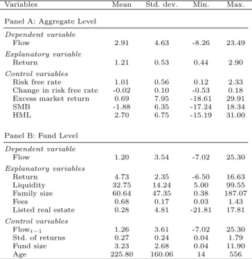
Table 1 presents descriptive statistics for fund flows, which is our key variable of interest, and for the explanatory variables over the 1990:3 to 2010:4 period. Furthermore, Table 1 contains the descriptive statistics of the employed control variables. Panel A shows the mean, standard deviation, minimum, and maximum for the quarterly aggregate level variables. Panel B shows the same metrics for the monthly fund level variables.
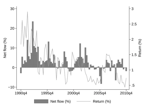
We first focus on the aggregate level statistics in Panel A of Table 1. On average, real estate funds experienced positive growth rates of 2.91% per quarter, in excess of the growth in AuM that is caused by positive returns. The standard deviation associated with these growth rates is 4.63%. The minimum net flow reveals a maximum loss of 8.26% of AuM in a single quarter, while the maximum value equates to a quarterly inflow of 23.49%. Over the same period, the average value-weighted quarterly return of all real estate funds is 1.21%, which equates to an annualized total return of 4.84%. Thus, the average return of real estate funds in excess of the risk free rate is 0.8% per year and, thus, substantially lower than the annualized excess return of the German stock market (2.76%). The standard deviation of quarterly returns of 0.53% indicates real estate funds are a low risk investment. The risk-return profile that should appeal to more risk-averse investors is complemented by a minimum quarterly return that is still positive (0.44%). In Figure 1, we plot aggregate flows and returns over the sample period. Flows are measured on the left vertical axis, returns are measured on the right vertical axis. Consistent with the correlation coefficients, the co-movement indicates that investors tend to invest more during times of high returns and less during periods of low returns.
Next, we turn to the descriptive statistics at the individual fund level in Panel B of Table 1.
As expected, the fund level numbers show a wider distribution compared to the aggregate level.
Even after winsorizing, we observe monthly outflows as high as -7.02% and maximum inflows into individual funds of more than 25% of AuM. The average monthly net flow into individual real estate funds is 1.2%, and thus higher than at the monthly equivalent at the aggregate level.
This suggests that smaller funds experience stronger growth relative to large funds.
The average 12-month return of the real estate funds in our sample (measured at a quarterly frequency) is 4.73% with a maximum of 16.63% and a minimum of -6.50%.6 The average fund family in our sample has 60.64 billion Euros in assets under management, whereby the largest fund family manages 187 billion Euros and the smallest fund family only 380 million Euros. The average expense ratio of the real estate funds in our sample is 0.68% per year.7
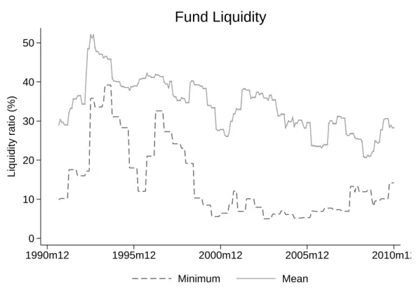
We observe substantial heterogeneity in the liquidity ratios of the funds in our sample. The average liquidity ratio is 32.75% with a standard deviation of 14.24%. The lowest liquidity ratio is 5.00% and therefore just above the critical value of 5%. The maximum liquidity ratio is 99.55%.
Liquidity ratios near 100% may occur for young funds which have already raised money, but
6 Note that fund level returns and their standard deviations refer to monthly measures of the total return over the previous twelve months, while all other variables refer to monthly data.
7Real estate specific fees for asset and property management are fund expenses and not paid directly by the investor. The relatively low fee for the real estate funds in our sample is likely due to scale economies and the fact that real estate funds are much larger than other asset funds. See Downs et al. (2015) for additional details on German open-end, direct-property funds.
Table 1:Descriptive statistics for aggregate and fund level variables
Variables Mean Std. dev. Min. Max.
Panel A: Aggregate Level Dependent variable
Flow 2.91 4.63 -8.26 23.49
Explanatory variable
Return 1.21 0.53 0.44 2.90
Control variables
Risk free rate 1.01 0.56 0.12 2.33
Change in risk free rate -0.02 0.10 -0.53 0.18
Excess market return 0.69 7.95 -18.61 29.91
SMB -1.88 6.35 -17.24 18.34
HML 2.70 6.75 -15.19 31.00
Panel B: Fund Level Dependent variable
Flow 1.20 3.54 -7.02 25.30
Explanatory variables
Return 4.73 2.35 -6.50 16.63
Liquidity 32.75 14.24 5.00 99.55
Family size 60.64 47.35 0.38 187.07
Fees 0.68 0.17 0.03 1.43
Listed real estate 0.28 4.81 -21.81 17.81
Control variables
Flowt−1 1.26 3.61 -7.02 25.30
Std. of returns 0.27 0.24 0.04 1.79
Fund size 3.23 2.68 0.04 11.90
Age 225.80 160.06 14 556
This table contains the descriptive statistics for the aggregate and fund level variables used throughout the analysis over the September 1990 to December 2010 period. Panel A shows the aggregate level variables:
Flow (%) = total absolute net flow of the quarter into all real estate funds divided by the total size of all real estate funds at the end of the previous quarter; Return (%) = value-weighted return of the quarter of all real estate funds; Risk free rate = Germany 3-month treasury bill rate in EUR; Change in risk free rate (%) = change in the Germany 3- month treasury bill rate in EUR; Excess market return (%) = Germany stock market return in excess of the risk free rate in EUR; SMB (%) = Germany small-firm minus big firm return factor in EUR; HML (%) = Germany high book-to-market minus low book-to-market return factor in EUR. Panel B shows the fund level variables: Flow (%) = absolute net flow of the month into the fund divided by fund size at the end of the previous month; Return (%) = fund return of the past 12 months;
Liquidity (%) = cash holdings of the fund divided by fund size; Family size (billions of EUR) = family size at the end of the month; Fees (%) = Expense ratio of the past 12 months; Listed real estate (%) = Monthly total return of the FTSE EPRA/NAREIT Developed Europe Index;
F lowt−1 = Flow into the fund in the previous month; Std. of returns (%) = fund return volatility of the past 12 months; Fund size (billions of EUR) = fund size at the end of the month; Age = fund age in months.
not yet closed any property transactions, so their assets only consist of cash holdings. Figure 2 graphs the mean and minimum liquidity ratio for the funds in our sample over the September 1990 to December 2010 period. Our final explanatory variable, the average monthly total return of the European listed real estate market is 0.28% with a minimum of -21.81% and a maximum of 17.81%.
Control variables include monthly fund flows lagged by one period, whereby the numbers are nearly identical compared to the dependent variable. The average real estate fund size is 3.23 billion Euros. The largest fund in our sample has a size of 11.90 billion Euros, which compares to a minimum fund size of only 37 million Euros. The average standard deviation of the 12-month
.5 1 1.5 2 2.5 3
Return (%)
−10 0 10 20 30
Net flow (%)
1990q4 1995q4 2000q4 2005q4 2010q4
Net flow (%) Return (%)
Fig. 1: This figure shows the time series of aggregate fund flows and returns of all real estate funds between September 1990 and December 2010.
return is characteristically low at 2.35%, which is part of the attraction of real estate funds for retail investors. The average fund age in our sample is close to 10 years (or 226 months).
Table 2, Panel A contains the contemporaneous correlations for the aggregate variables. A star indicates that the correlation is statistically significant at the 5% level. The first column in Panel A reveals a positive and statistically significant correlation between aggregate flows and returns (ρ=0.42). The respective correlation coefficient between flows and lagged returns is even stronger (ρ=0.53). This suggests fund flows may follow returns. The second column of Panel B contains the correlation coefficients between returns and lagged flows. Returns are positively correlated with past flows (ρ=0.23).
The strong and statistically significant correlation between flows and lagged flows (ρ=0.50) in the first column of Panel B and, likewise, the positive correlation between returns and lagged returns (ρ=0.71) in the second column of Table B indicate that our main variables of interest are autocorrelated and may follow a unit root process. However, our tests reject the null hypothesis that these time series contain a unit root, so we include these variables without modifications.
Fund flows are positively correlated with both, the contemporaneous (ρ=0.35) and the lagged level (ρ=0.47) of the risk free rate. This suggest investors tend to buy real estate funds during times of high interest rates. However, this positive relationship may also be driven by the fact that periods of high real estate returns coincide with high levels of the risk free rate (ρ=0.84). In contrast, aggregate flows into real estate funds are negatively correlated with contemporaneous (ρ=-0.41) and lagged (ρ=-0.42) changes in the risk free rate. The correlations between returns
0 10 20 30 40 50
Liquidity ratio (%)
1990m12 1995m12 2000m12 2005m12 2010m12
Minimum Mean
Fund Liquidity
Fig. 2:This figure shows the mean and minimum liquidity ratios.
Table 2: Contemporaneous and lagged correlations for aggregate variables
Flow Return RF DRF MKTRF SMB HML
Panel A: Contemporaneous correlations
Flow 1 - - - - - -
Return 0.42* 1 - - - - -
Risk free rate (RF) 0.35* 0.84* 1 - - - -
Change in risk free rate (DRF) -0.41* -0.00 0.01 1 - - -
Excess market return (MKTRF) 0.06 -0.15 -0.27* 0.06 1 - -
SMB 0.07 -0.15 -0.09 -0.14 0.36* 1 -
HML -0.12 -0.10 -0.10 0.10 -0.04 -0.26* 1
Panel B: Lagged correlations
Flowt−1 0.50* 0.23* 0.31* -0.23* 0.08 0.01 -0.13
Returnt−1 0.53* 0.71* 0.83* -0.13 -0.17 -0.06 0.02
Risk free rate (RF)t−1 0.47* 0.82* 0.98* -0.17 -0.29* -0.07 -0.09
Change in risk free rate (DRF)t−1 -0.42* 0.09 0.13 0.57* -0.25* -0.09 0.02
Excess market return (MKTRF)t−1 -0.09 -0.19 -0.22 0.25* 0.18 0.28* -0.01
SMBt−1 -0.19 -0.24* -0.07 0.13 0.17 0.27* -0.01
HMLt−1 0.03 -0.06 -0.10 -0.03 -0.12 -0.05 -0.16
Flow (%) = total absolute net flow of the quarter into all real estate funds divided by the total size of all real estate funds at the end of the previous quarter; Return (%) = value-weighted return of the quarter of all real estate funds; Risk free rate (RF) (%) = Germany 3-month treasury bill rate in EUR; Change in risk free rate (%) = change in the Germany 3-month treasury bill rate in EUR; Excess market return (%) = Germany stock market return in excess of the risk free rate in EUR; SMB (%) = Germany small-firm minus big firm return factor in EUR; HML (%) = Germany high book-to-market minus low book-to-market return factor in EUR. * denotes significance at the 5% level.
and changes of the risk free rates (i.e., contemporaneous as well as lagged), are not statistically significant.
4 Aggregate Flows and Returns
4.1 Vector Autoregression (VAR) Methodology
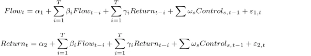
In this section, we empirically test whether investors chase past returns (Hypothesis 1). We also examine whether they possess market timing ability or, alternatively, whether aggregate flows have a performance diluting effect. We employ VAR methodology to examine the dynamic relationship between aggregate flows and returns of real estate funds. A VAR model is a system of simultaneous equations where the dependent variables are expressed as linear functions of their own and each other’s lagged values and exogenous variables. Several specifications of the following VAR model are estimated:
F lowt=α1+
T
X
i=1
βiF lowt−i+
T
X
i=1
γiReturnt−i+X
ωsControls,t−1+ε1,t (3)
Returnt=α2+
T
X
i=1
βiF lowt−i+
T
X
i=1
γiReturnt−i+X
ωsControls,t−1+ε2,t (4)
F lowtis the net absolute flow into all real estate funds divided by the total fund volume of the previous period.Returntis the value-weighted return of all real estate funds.
Our set of exogenous control variables includes the lagged change in the risk free rate. All else being equal, we expect that interest rate increases reduce flows into real estate funds. The reasons are two-fold. First, given the risk-return characteristics of real estate funds are relatively similar to those of the risk free rate, the two investments may be seen as alternatives by investors seeking diversification. An increase in the risk free rate would decrease the relative attractiveness of real estate funds. Second, interest rate increases usually have a negative impact on direct property prices. This might be anticipated by real estate fund investors and, hence, provides an incentive to withdraw their money from real estate funds. We also control for the level of the risk free rate as it has an effect on the performance of real estate funds due to their large cash holdings. Finally, we control for capital market factors that may have an effect on returns and investor behavior by including the three Fama-French risk factors (Market excess return, SMB, HML).ε1,t andε2,t are innovations that may be contemporaneously correlated with each other, but are uncorrelated with their own lagged values and uncorrelated with all of the right-hand side variables.
The unconstrained VAR system is estimated with quarterly data for the 1992q1 to 2010q4 period. We sequentially estimate models with up to six lags and use Akaike information crite- rion, Schwarz information criterion, and Hannan-Quinn information criterion as model selection criteria. We find four lags satisfies the criteria.
4.2 VAR Results
Table 3 summarizes our results from the VAR analysis. We estimate five different specifications.
Model (i) is our base case, where the analysis is restricted to the endogenous variables only. In model (ii), we add the lagged change of the risk free rate as an exogenous control variable and in model (iii), we use the absolute level of the risk free rate at the end of the previous quarter. In model (iv), we simultaneously control for measures of the risk free rate. In model (v) we built up
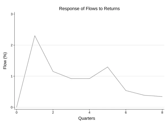
0 1 2 3
0 2 4 6 8
Response of Flows to Returns
Flow (%)
Quarters
Fig. 3:This figure shows the response of aggregate real estate fund flows to returns based on model (v) of Table 3.
on model (iv) by including the three country-specific, Fama-French risk factors. The first column of each model refers to the flow equation, while the second column refers to the return equation of the VAR.
We first turn to the flow equations of the five models in order to examine whether investors chase past returns (Hypothesis 1). The results in the first columns of model (i) reveal the returns of real estate funds predict aggregate real estate fund flows beyond past flows. Although, none of the four lagged coefficients is individually significant, a joint test of the lagged returns on flows is positive and statistically different from zero. The sum of the four lagged coefficients on return is 5.09 with a z-statistic of 4.60. This effect remains robust even after including the various exogenous control variables in models (ii) to (v). Thus, our results are consistent with return chasing behavior of real estate fund investors at the aggregate level.
The graphical analysis of impulse response functions provides further insights about the short- and long term relationship between flows and returns. Figure 3 plots the response of quarterly aggregate fund flows to a one standard deviation return shock. The graph shows a strong reaction of flows in the quarter that follows the shock. The effect of the return shock is persistent, yet partially reduced after the second quarter until the effect finally dissipates after 6 quarters. The results are based on model (v).
Our results also indicate aggregate flows are serially correlated. In model (i), the estimated coefficient of flows on flows in the previous quarter is positive and statistically different from zero, suggesting that aggregate flows are autocorrelated in the short term. The second and third lag are insignificant, but flows are also autocorrelated with their fourth lag. The sum of the four
Table3:Vectorautoregressionresultsforaggregateflowsandreturns (i)(ii)(iii)(iv)(v) FlowtReturntFlowtReturntFlowtReturntFlowtReturntFlowtReturnt Flowt−10.239**-0.018**0.096-0.0080.200*-0.0090.093-0.0040.136-0.003 (2.28)(-1.98)(0.92)(-0.82)(1.85)(-1.05)(0.88)(-0.41)(1.32)(-0.38) Flowt−2-0.023-0.0090.023-0.012-0.038-0.0050.020-0.0080.024-0.011 (-0.21)(-0.91)(0.22)(-1.32)(-0.35)(-0.59)(0.19)(-0.95)(0.24)(-1.31) Flowt−3-0.193*0.019**-0.201**0.020**-0.197*0.020**-0.201**0.021**-0.218**0.023*** (-1.78)(2.05)(-2.00)(2.23)(-1.84)(2.32)(-2.00)(2.40)(-2.22)(2.76) Flowt−40.302***-0.027***0.277***-0.025***0.293***-0.025***0.276***-0.024***0.311***-0.024*** (3.12)(-3.24)(3.08)(-3.18)(3.05)(-3.21)(3.07)(-3.18)(3.61)(-3.23) Returnt−11.4000.391***2.633**0.301***2.2230.204*2.727**0.1782.304*0.107 (1.19)(3.81)(2.30)(2.95)(1.64)(1.84)(2.14)(1.63)(1.86)(1.01) Returnt−20.9070.1501.1720.1311.680-0.0251.274-0.0040.593-0.011 (0.74)(1.40)(1.03)(1.29)(1.22)(-0.22)(0.99)(-0.03)(0.47)(-0.10) Returnt−30.8940.203*0.2990.246**1.5560.0530.3990.1140.6620.110 (0.75)(1.95)(0.27)(2.47)(1.19)(0.49)(0.31)(1.05)(0.55)(1.07) Returnt−41.8920.250**1.1330.305***2.359*0.1441.2090.205**1.0230.173* (1.58)(2.40)(1.00)(3.03)(1.89)(1.41)(0.99)(1.97)(0.88)(1.74) Changeinriskfreeratet−1---14.287***1.038***---14.061***0.739**-15.267***0.533 --(-3.56)(2.91)--(-3.33)(2.05)(-3.72)(1.52) Riskfreeratet−1-----2.2640.514***-0.3110.411***0.2060.503*** ----(-1.21)(3.35)(-0.17)(2.61)(0.11)(3.23) MarketExcessReturnt−1--------0.0150.007* --------(0.30)(1.69) SMBt−1---------0.125**-0.015*** --------(-2.11)(-2.91) HMLt−1--------0.078-0.002 --------(1.49)(-0.42) Constant-0.042***0.001-0.043***0.001-0.051***0.003**-0.044***0.002**-0.044***0.002** (-3.58)(0.61)(-3.94)(0.70)(-3.70)(2.35)(-3.38)(2.06)(-3.50)(2.24) Observations77777777777777777777 R-squared51.666.958.470.2152.571.158.472.663.075.1 SumofFlow0.325**-0.035***0.195-0.025**0.258*-0.0200.188-0.0160.254*-0.015 (2.21)(-2.71)(1.39)(-2.01)(1.66)(-1.53)(1.28)(-1.26)(1.78)(-1.25) SumofReturn5.094***0.994***5.237***0.984***7.82***0.376*5.609**0.492**4.583*0.380* (4.60)(10.33)(5.10)(10.77)(3.12)(1.83)(2.30)(2.37)(1.96)(1.89) Thistablecontainsthevectorautoregression(VAR)resultsforthe1992q1-2010q4periodwiththeendogenousvariablesnetflow(%)andreturn(%),whileall othervariablesentertheequationasexogenouscontrols.Netflow(%)isthetotalmoneyflowintoallrealestatefundsdividedbytotalassetsundermanagement ofallrealestatefundslaggedbyonequarter.Return(%)isthevalue-weightedtotalreturnofallrealestatefunds.Changeinriskfreerate(%)isthequarterly changeintheGermany3-monthtreasurybillrateinEUR.TheriskfreerateistheGermany3-monthtreasurybillrateinEUR.Excessmarketreturn(%)is theGermanystockmarketreturninexcessoftheriskfreerateinEUR.SMB(%)istheGermanysmall-firmminusbigfirmreturnfactorinEUR.HML(%) istheGermanyhighbook-to-marketminuslowbook-to-marketreturnfactorinEUR.T-statisticsareinparentheses.Coefficientsmarkedwith***,**and*are significantatthe1%,5%,and10%level,respectively.
lagged coefficients on flow is 0.33 and statistically significant at the 5% level. Overall, a simple, bivariate model (i) explains 51.6% of the variation of aggregate flows. The joint significance of the four lagged flow coefficients disappears in models (ii) to (iv), where we control for the risk free rate, but is significant again in model (v), where we additionally control for the Fama-French risk factors.
The results of the flow equation in model (ii) show strong evidence that aggregate flows are negatively related to lagged changes in the risk free rate. This effect is robust to the inclusion of further control variables in models (iv) and (v) and supports the view that real estate funds are less attractive for investors when interest rates rise. This may either be the case because substitute investments, such as money market funds, become more attractive or because of the negative effect of interest rate increases on property prices and, hence, on anticipated returns of real estate funds. We find no significant relationship between aggregate flows and the level of the risk free rate. Furthermore, aggregate flows are negatively related to the SMB-factor, but positively related to the HML-factor. Thus, flows into real estate funds are higher when large stocks do better than small stocks and when stocks with a high book-to-market ratio outperform stocks with a low book-to-market ratio. Finally, the R-squared of model (v) is 63%.
Next, we turn to the return equations in order to test whether aggregate flows are predictive of aggregate returns. Overall, we find no evidence of a positive relationship between aggregate returns and past flows. There is a positive effect of the third lag of flows on returns and this effect is robust across all five models. However, the sum of the four lagged coefficients on flow is not positive in any of the models. Fund flows might also dilute returns by increasing a fund’s low-yield cash holdings. In models (i) and (ii), the overall effect of flow on return is negative and statistically significant, which is consistent with a performance diluting effect of flows on returns.
However, this effect is no longer significant in models (iii) to (v), as additional exogenous control variables are introduced.
We find strong evidence that aggregate returns are serially correlated. In model (i), the sum of the four lagged return coefficients is 0.99 with a z-statistic of 10.33. The magnitude of the overall effect is reduced by more than 50%, but remains significant in models (iii) to (v). This suggests that the level of the risk free rate is an important determinant of aggregate real estate fund returns. In model (iii), the level of the lagged risk free rate has a coefficient of 0.51 and is statistically different from zero. This result reflects that the large cash holdings of real estate funds are an important determinant of their performance. Furthermore we find that aggregate real estate returns are positively related to lagged changes in the risk free rate and the lagged stock market excess return, and negatively related to the lagged SMB factor (i.e., the returns of real estate funds are higher when large caps outperform small cap stocks).
5 Individual Fund Flows and Returns
5.1 Piecewise Linear Regression Methodology
In this section, we analyze the flow-performance relationship for real estate at the individual fund level. We follow Sirri and Tufano (1998) and examine the shape of the flow-performance relationship using a piecewise linear regression methodology. This approach allows for different flow-performance sensitivities for different levels of performance. In each month, we rank all real estate funds by their performance over the previous 12 months from zero (worst performance) to
one (best performance), where the ranks correspond to the fund’s performance percentile.8Based on their performance percentile, funds are classified into low, medium and high performance using the following decomposition:9
Lowi,t=min(0.2, Ranki,t)
M idi,t=min(0.6, Ranki,t−Lowi,t) Highi,t=Ranki,t−(Lowi,t+M idi,t)
(5)
Lowi,t represents the performance rank for funds in the bottom 20% of the distribution.
M idi,t represents the performance rank of funds whose performance percentile falls into the range of 20% to 80%, andHighi,t represents the performance rank for the 20% of funds with the best performance. We then regress monthly fund flows on the first lags of these fractional rank variables, where their coefficients represent the slope of the flow-performance relationship over their range of sensitivity:
F lowi,t=α1+β1Lowi,t−1+β2M idi,t−1+β3Highi,t−1 +δtT imeDummyt+X
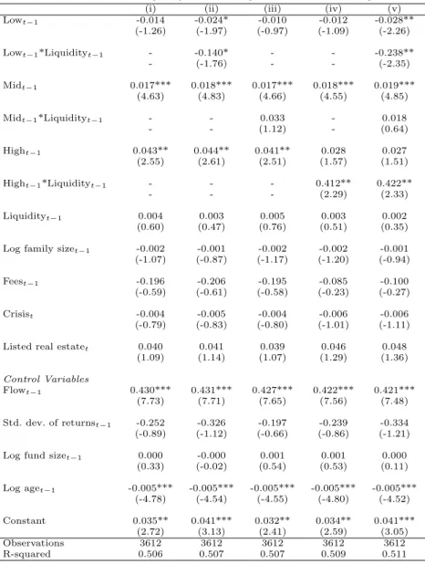
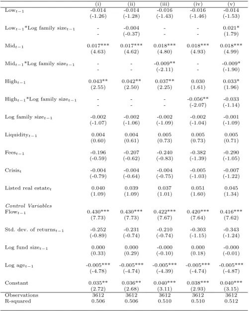
ωsControli,t−1+εi,t
(6) To examine the impact of fund liquidity on the shape of the flow-performance relationship (Hypothesis 2), we interact performance with the liquidity ratio of the fund. To test whether the flow-performance relationship of real estate funds is sensitive to participation costs (Hypothesis 3), past performance is interacted with our proxies for participation costs: fund fees and the natural logarithm of fund-family size.
We de-mean the interacted variables across time to preserve the interpretability of the slope coefficients. Without modifications the coefficient on the fractional performance variables would correspond to the partial derivative of flows with respect to the performance variable when the proxy variable is zero. Of course, a liquidity ratio of zero is implausible. De-meaning the interacted variables ensures the interpretation of the coefficient on the explanatory variable is the same as it would be without the interaction (Balli and Sorensen, 2013).
Previous studies document that fund flows are also affected by non-performance related vari- ables. Beyond past performance, lagged flows into the fund, the fund’s riskiness, the size of the fund and fund age all help to determine which mutual funds investors prefer (Patel et al. 1991;
Jain and Wu 2000; Kempf and Ruenzi, 2008). We control for possible autocorrelation in the dependent variable by including lagged flows (F lowi,t−1). Furthermore, we include the lagged risk of the fund, measured by the standard deviation of the fund’s monthly total returns over the previous twelve months (Std.dev.of returnsi,t−1), the natural logarithm of the size of the fund at the end of the previous month (LogF undsizei,t−1), and the natural logarithm of the age of fund(LogAgei,t−1).
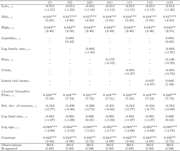
5.2 Convexity of the Flow-Performance Relationship for Real Estate Funds
Table 4 contains the regression results on the flow-performance relationship for individual real estate funds over the September 1990 to December 2010 period. Seven different specifications are estimated. In model (i), we estimate the flow-performance relationship controlling fund flows
8At the request of an anonymous referee, we conduct robustness tests by ranking funds based on risk-adjusted performance using one-factor and four-factor alphas. Overall, our results are stable to using these alternative ranking procedures. The results are available from the authors upon request.
9In untabulated results, we obtain consistent results using a more conservative approach for the performance decomposition.