Band 76
Christian Witt
Essays
on Real Estate and Financial Crisis
From the US Housing Market Downturn to the Global Financial Crisis
Schriften
zu Immobilienökonomie und Immobilienrecht
Herausgeber:
IRE
I
BS International Real Estate Business SchoolProf. Dr. Sven Bienert
Prof. Dr. Stephan Bone-Winkel Prof. Dr. Kristof Dascher Prof. Dr. Dr. Herbert Grziwotz Prof. Dr. Tobias Just
Prof. Gabriel Lee, Ph. D.
Prof. Dr. Kurt Klein
Prof. Dr. Jürgen Kühling, LL.M.
Prof. Dr. Gerrit Manssen
Prof. Dr. Dr. h.c. Joachim Möller Prof. Dr. Wolfgang Schäfers
Prof. Dr. Karl-Werner Schulte HonRICS Prof. Dr. Steffen Sebastian
Prof. Dr. Wolfgang Servatius Prof. Dr. Frank Stellmann Prof. Dr. Martin Wentz
Witt, Christian
Essays on Real Estate and Financial Crisis
From the US Housing Market Downturn
to the Global Financial Crisis
Die Deutsche Bibliothek – CIP Einheitsaufnahme
Witt, Christian
Essays on Real Estate and Financial Crisis
Regensburg: Universitätsbibliothek Regensburg 2015
(Schriften zu Immobilienökonomie und Immobilienrecht; Bd. 76) Zugl.: Regensburg, Univ. Regensburg, Diss., 2015
ISBN 978-3-88246-357-6
ISBN 978-3-88246-357-6
© IRE|BS International Real Estate Business School, Universität Regensburg Verlag: Universitätsbibliothek Regensburg, Regensburg 2015
Zugleich: Dissertation zur Erlangung des Grades eines Doktors der Wirtschaftswissen- schaften, eingereicht an der Fakultät für Wirtschaftswissenschaften der Universität Re- gensburg
Tag der mündlichen Prüfung: 28.Mai 2014 Berichterstatter: Prof. Dr. Steffen Sebastian
Prof. Dr. Enzo Weber
Acknowledgements
Without the encouragement of my family, supervisors, colleagues and friends, I would have never gotten this far. So, please let me express my gratitude to all those who helped me in the process of finishing my dissertation.
First and foremost, I am indebted to my wife Eug´enie, to my parents Kerstin and Uwe, to my sister Katharina, to my parents-in-law Josselyne and Henri, and to Heidi David for all your patience and moral support. You were always there for me.
Moreover, I would like to sincerely thank my two supervisors Prof. Dr. Steffen Sebastian and Prof. Dr. Enzo Weber. Your help was priceless. Not only did you teach me my first lessons about how to perform research, but also always shared your critical mind and constructive suggestions. An extra thank you to Prof. Dr. Sebastian for having been a great mentor. You were the one offering me this outstanding opportunity. You facilitated my research stay abroad. You granted me a maximum of academic freedom.
You provided me with guidance whenever needed. Last but not least, you were my fellow co-author on “Two Sides of the Same Coin? Financial Integration vs. Financial Integration” (Chapter 3).
I am further grateful to my second co-author Dr. Frank Hespeler for your great cooper- ation. Beyond contributing to “The Systemic Risk Dimension of Hedge Fund Illiquidity and Prime Brokerage” (Chapter 2) you always took the time for controversial discussions and to teach me more about pitfalls in econometric analysis.
Finally, my dearest thanks go out to all the people commenting on various ideas and draft versions of the three chapters. Time and again you have lend me an open ear al- lowing me to mirror, sort out and develop my own thoughts: Patrick Armstrong, Antoine Bouveret, Thomas Braun, Oliver Burkart, Marcelo Cajias, Laurent Degabriel, Benedikt Fleischmann, Peter Geiger, Oliver Gilvarry, Stefan Glossner, Ralf Hohenstatt, Steffen
Kern, Tim Koniarski, Christoph Memmel, Albert Menkveld, Tarun Ramadorai, Verena Ross, Bertram Steininger and Christian W¨altermann, two anonymous referees, as well as seminar participants at the European Financial Markets Association, European Real Estate Society, European Securities and Markets Authority (ESMA), German Finance As- sociation, HVB Doctoral Seminar, IREBS Doctoral Seminar, Swiss Society for Financial Market Research, WHU Campus for Finance and ZEW Real Estate and Capital Markets Network.
Christian Witt
Regensburg, 28 May 2014
Contents
Contents iv
List of Figures vi
List of Tables vii
List of Acronyms viii
Preface 1
1 On Housing Market Downturns and Optimal Seller Behaviour 5
1.1 Introduction . . . 6
1.2 Homogeneous Housing Market . . . 11
1.2.1 Static Equilibrium . . . 11
1.2.2 Housing Market Downturns . . . 13
1.3 Heterogeneous Housing Market . . . 17
1.3.1 Static Equilibrium . . . 18
1.3.2 Housing Market Downturns . . . 19
1.4 Simulation Analysis . . . 26
1.4.1 Homogeneous Housing Market . . . 28
1.4.2 Heterogeneous Housing Market . . . 28
1.4.3 Cross-Segment Competition and Shock Co-Movement . . . 32
1.4.4 Influencing Seller Behaviour . . . 34
1.5 Revisiting the 2006-09 US Housing Market Crash . . . 36
1.5.1 Non-Recourse Financing and Credit Quality . . . 36
1.5.2 Mortgage Losses and House Prices . . . 40
1.6 Conclusions . . . 43
2 The Systemic Dimension of Hedge Fund Illiquidity and Prime Broker- age 48 2.1 Introduction . . . 49
2.2 Data . . . 51
2.2.1 Hedge Funds — an Illiquidity Premium . . . 52
2.2.2 Prime Brokers . . . 53
2.2.3 Macroeconomic and Financial Control Variables . . . 54
2.2.4 Turmoil Control Variables . . . 54
2.3 Model Selection . . . 55
2.4 The Dynamic Interaction of Hedge Fund Illiquidity and Prime Brokerage . 60 2.4.1 In Periods with no Stress in Financial Markets, Hedge Funds and Prime Brokers Act as Complementary Trading Partners. . . 60
2.4.2 In the Short Run, Excess Returns on Prime Brokerage and Hedge Fund Illiquidity are Mainly Determined by Asset and Commodity Prices and Perceived Financial Risks. . . 63
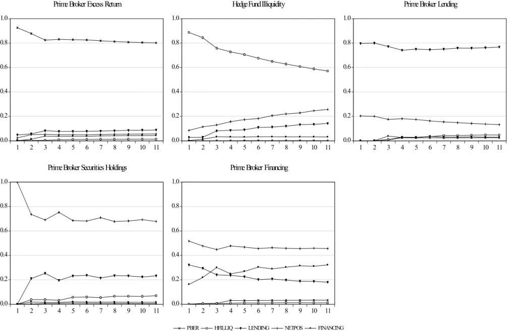
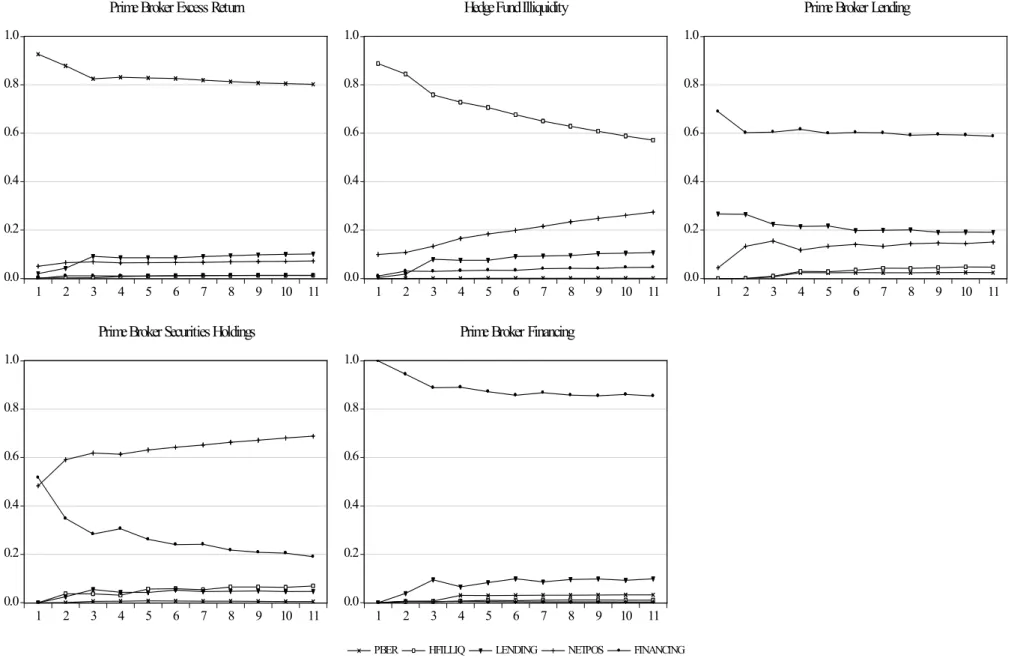
2.4.3 High Levels of Stress in Financial Markets Tend to Weaken the Intermediation Chain, since Prime Brokers Start to Hoard Liquid Securities. . . 64
2.4.4 Disruptions in the Financial Intermediation Chain Force Hedge Funds to Deleverage. . . 67
2.4.5 Adverse Shocks to any Element of the Intermediation Chain Impair the Profitability of Hedge Funds Stronger than the one of Prime Brokers. . . 74
2.5 Robustness checks . . . 75
2.6 The collapse of the financial intermediation via prime brokers and hedge funds during the recent financial crisis . . . 79
2.7 Conclusions . . . 82
3 Two Sides of the Same Coin? Financial Integration vs. Financial Con- tagion 84 3.1 Introduction . . . 85
3.2 Data . . . 88
3.3 Modelling Financial Sector Co-movement . . . 89
3.3.1 The Three-Factor Asset Pricing Model . . . 90
3.3.2 The Dynamic Conditional Correlation Model . . . 91
3.3.3 Correlation Components . . . 93
3.4 Financial Integration and Financial Contagion . . . 94
3.4.1 The Role of Common Shocks . . . 95
3.4.2 The Role of Extreme Events and Repo Market Failure . . . 99
3.4.3 The Role of Contagion and Flight-to-Quality in Financial Integration102 3.5 Conclusions . . . 110
Bibliography 112
A Housing Market Downturns 121
B Hedge Funds and Prime Brokers 124
C Financial Sector Integration 127
List of Figures
1.1 US house prices and home sales . . . 7
1.2 Course of events . . . 13
1.3 Housing market dynamics . . . 14
1.4 Decision problem in homogeneous housing market . . . 17
1.5 Decision problem in heterogeneous housing market . . . 22
1.6 Homogeneous housing market . . . 29
1.7 Heterogeneous housing market . . . 30
1.8 Cross-segment competition and shock-co-movement . . . 33
1.9 Policy interventions . . . 35
1.10 Foreclosures and house prices . . . 38
1.11 Mortgage losses and house prices . . . 41
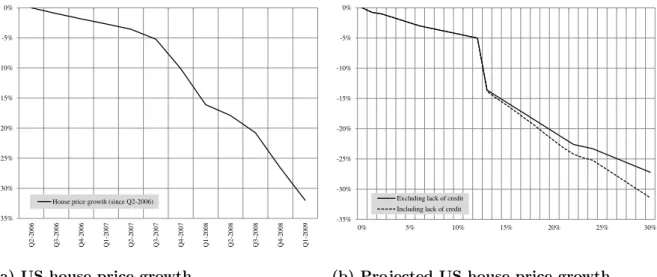
1.12 Observed and projected US house price growth . . . 43
2.1 Impulse responses . . . 66
2.2 Risk shock (prime broker financing) . . . 68
2.3 Risk shock (prime broker lending) . . . 69
2.4 Shocks to hedge funds . . . 72
2.5 Shocks to money markets . . . 73
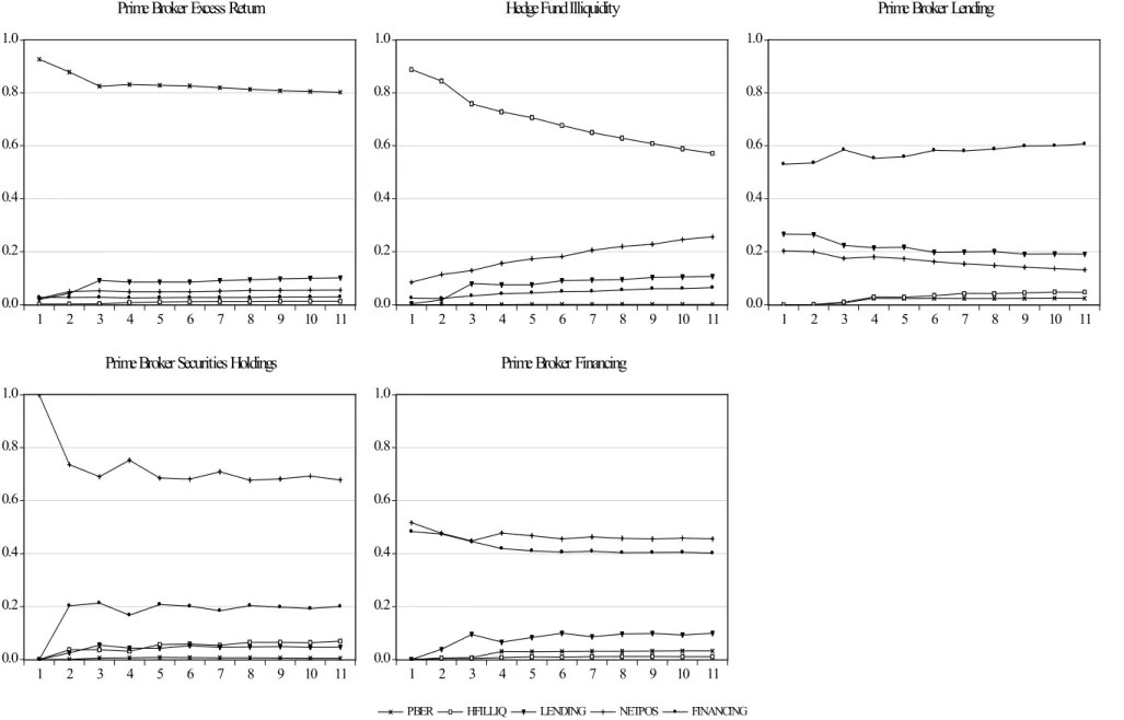
2.6 Model fit and parameter stability . . . 76
2.7 Indirect proxies of parameter stability . . . 77
2.8 Modified variable constructions and omitted variables . . . 78
3.1 Unconditional coefficients . . . 97
3.2 Crisis-related shifts . . . 98
3.3 DCC- and DCCX-implied correlation dynamics . . . 101
3.4 Aggregate correlations . . . 104
3.5 US, global and domestic correlation components . . . 105
3.6 Residual correlation component . . . 106
3.7 Contagion and flight-to-quality in the Subprime Crisis . . . 108
3.8 Contagion and flight-to-quality in the Euro Crisis . . . 109
A.1 Cross-segment competition . . . 122
A.2 Shock co-movement . . . 123
C.1 Auxiliary regressions . . . 127
C.2 DCCX vs. DCC correlations . . . 128
C.3 DCCX-implied residual correlations . . . 129
List of Tables
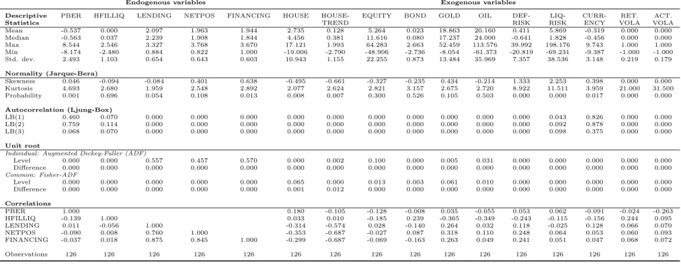
2.1 Data characteristics . . . 56
2.2 Selection of VEC model . . . 57
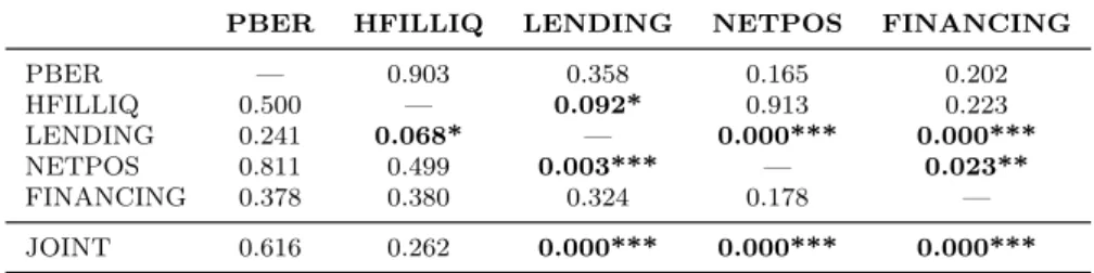
2.3 Granger causality . . . 59
2.4 VEC model estimates . . . 62
3.1 Panel three-factor asset pricing model . . . 96
A.1 Model parameterization . . . 121
B.1 Prime broker details . . . 125
B.2 Variable definitions and sources . . . 126
C.1 Variables and sources . . . 130
C.2 Data characteristics . . . 131
C.3 Individual three-factor asset pricing model . . . 133
C.4 Auxiliary regressions . . . 135
C.5 Residual variances . . . 136
C.6 Time-varying residual correlations . . . 137
C.7 Correlation decomposition . . . 138
C.8 Correlation decomposition regressions . . . 140
List of Acronyms
ABCP Asset-Backed Commercial Paper: A short-term security backed by a pool of financial assets. Maturities range up to 270 days. Typical collateral involves mortgages, credit-card receivables, leases, royalties, car or student loans.
ABS Asset-Backed Security: A security backed by a pool of financial as- sets other than real estate and mortgages. Typical collateral involves credit-card receivables, leases, royalties, car or student loans.
AuM Assets under Management.
BBA Britisch Bankers Association.
CDO Collateralised Debt Obligation: A structured financial product used to repackage and securitise other financial assets. Typical collat- eral involves asset-backed securities, corporate loans, leveraged loans, mortgage-backed securities, or project finance debt.
CDS Credit Default Swap: A swap agreement designed to offer the buyer an insurance against the default risk of an underlying asset. Under the agreement the seller compensates the buyer in the event the underlying loan experiences a pre-defined credit event. The buyer periodically pays a premium in return, unless a credit event takes place.
DCC Dynamic conditional correlation.
DCCX Dynamic conditional correlation including exogenous variables.
Factor DCCX Factor dynamic conditional correlation including exogenous variables.
FRBNY Federal Reserve Bank of New York.
GARCH Generalised autoregressive conditional heteroskedasticity.
IMF International Monetary Fund.
LIBOR London Interbank Offered Rate.
LTCM Long-Term Capital Management.
LTV Loan-to-Value ratio: A financial ratio used in the real estate sector.
It illustrates the leverage a debtor obtains by borrowing against a property.
MBS Mortgage-Backed Security: A security backed by a pool of mortgages or other real estate loans.
MSCI Morgan Stanley Capital International.
Repo Repurchase Agreement: A financial transaction designed to facilitate borrowing against other liquid securities, such as government bonds or equities. Under the agreement the original seller promises to later buy back the security at a pre-defined higher repurchase price. This way the transaction effectively constitutes a fixed-rate secured loan, where the seller functions as the borrower and the buyer as the lender.
SIFI Systemically Important Financial Institution: A bank, insur- ance or other financial institution whose “insolvency would have a serious impact on the functioning of the domes- tic financial system or significant parts thereof, and would also have negative effects on the real economy” (Bundes- bank: http://www.bundesbank.de/Navigation/DE/Service/Glossar/
Functions/glossar.html?lv2=129548&lv3=146026)
UK United Kingdom.
US United States of America.
VEC Vector error correction.
“Is [the recent mortgage slowdown] a mere irritant in America’s vast economy, or the start of something much worse? Opinion on Wall Street is divided. Most argue that the mortgage mess, though a blight on anyone caught up in it, will not spread. The number of mortgages at risk is too small for defaults to threaten everyone else.”
The Economist, “Cracks in the fa¸cade”, 22 March 2007.
Preface
If you were to ask an economist what the period 2007 to 2009 was all about, the probable answer would be that this was the time of the Global Financial Crisis, one of the most severe episodes of financial stress since the Great Depression. The respondent would be likely to continue that it all started with plummeting house prices in the US, which first spilled over into global interbank markets before triggering a near-meltdown of the world financial system. The repercussions eventually caused many economies around the globe to fall into a sharp recession.
This condensed r´esum´e portrays today’s reading of the Global Financial Crisis very well.
However, as with every summary, it hides some of the underlying stories that add up to the bigger picture. This is why this dissertation project seeks to address three elements of the chain of events that might deserve more careful attention. The selection is driven by one key question: how could a downturn in a rather small segment of the US housing market turn into a large-scale global financial crisis? In other words, the common theme of the analysis is the dissemination of the economic source shock across markets and regions. For reasons of clarification we distinguish three major phases of propagation: (i) the spreading from the US “subprime” housing market to the country’s entire residential real estate market; (ii) the proliferation across large banks and investors via secured money markets;
and (iii) the dissemination of financial turbulence across domestic financial sectors.
The first and barely noticed sign of an imminent crisis appeared in September 2006. The prices of US residential houses had just started to slide, in particular in the so-called
“subprime” market. This segment is characterised by the typically lower creditworthi-
ness and higher leverage of homeowners compared with the traditional “prime” segment (cf. Frame et al., 2008; Mian et al., 2009; Demyanyk and van Hemert, 2011). In many cases, the original decline drove market prices below the value of outstanding mortgages (Duke, 2012). Since residential mortgages are mostly non-recourse in the US, the affected homeowners had an incentive to default on their obligations voluntarily (Harris, 2010).
This incentive unfolded a wave of uncoordinated foreclosures. A vicious circle ensued, in which lower prices led to higher foreclosures, which reinforced the initial price drop (cf. Campbell et al., 2011; Frame et al., 2008; Mian et al., 2014). At this point, the down- ward spiral spilled over and harmed the prices of unforced sales (Campbell et al., 2011) in the “prime” segment. These homeowners chose to postpone a sale in order to preserve their long-run profitability. Hence, the overall home sales including both “prime” and
“subprime” became increasingly dominated by the worst-performing segment (cf. Wall Street Journal, 2009; CoreLogic, 2010). Chapter 1 examines the observed market dynam- ics from a game-theoretical perspective. The developed model explains several stylised facts of the recent US housing market crash. The analysis concludes that homeowners usu- ally postpone home sales during a market downturn to escape its negative consequences.
However, the typical non-recourse financing of residential real estate in combination with high leverage temporarily damaged the usual market mechanism. This paved the way for the subsequent nationwide housing crisis. On the other hand, the interventions pol- icy makers pursued to find a way out of the crisis (e.g. loose monetary policy, financial stimuli, urban planning) are consistent with the attempt to restore this mechanism.
How could turmoil in the US housing market spread further towards financial markets?
Recent research guides us to look into short-term secured funding markets (cf. Brun- nermeier, 2009; Gorton and Metrick, 2012): with house prices deteriorating, short-term obligations holding houses as collateral lost value, too. Short-term secured funding was squeezed as a result in the autumn of 2007 (Brunnermeier, 2009). Given the material dependence of market participants on this funding source prior to the crisis (cf. Allen and Carletti, 2008; Gorton and Metrick, 2012), the implications for this and related market segments were grave. The borrowing rates peaked, thereby aggravating the initial funding problems while creating further uncertainty and scepticism among the market participants with respect to the creditworthiness of their counterparties (cf. Allen and Carletti, 2008;
Brunnermeier, 2009; Taylor and Williams, 2009; Gorton and Metrick, 2012;). Hedge funds and prime brokers are traditionally the key players involved in short-term securities
borrowing and lending (Gorton and Metrick, 2012). The analysis of Chapter 2 therefore concentrates on the consequences of adverse shocks for this particular financial inter- mediation chain. The results demonstrate that the intermediation activity diminished significantly in periods of exceptionally high levels of uncertainty. The reduction itself seems to have been driven primarily by the securities hoarding of prime brokers trying to preserve their liquidity position. On top of this, rises in prime brokers’ securities hold- ings show the most devastating impact on financial intermediation activity among all the investigated shocks. Hence, the turmoil in the US housing market spread to short-term funding markets through plummeting collateral values, which caused prime brokers to build up precautionary security buffers at the cost of impaired financial intermediation activity.
After the collapse of the investment bank Lehman Brothers on 15 September 2008, the financial turmoil that had recently been limited to money markets suddenly spilled over and endangered entire domestic financial sectors around the globe (cf. Brunnermeier, 2009;Eichengreen et al., 2009; Bekaert et al., 2014). The Global Financial Crisis was born. Chapter 3 investigates the sources of this unanticipated and forceful global propa- gation of financial turbulence. As the analysis reveals, even elaborate factor asset pricing models are insufficient to describe the most severe episodes of the Global Financial Cri- sis. Further taking into account continuous time-dependent co-movement patterns adds precious information. Not only does it help to identify contagion—defined as residual co-movement unaccounted for by fundamentals—, but it also allows us to quantify its magnitude and to detect timing patterns. Indeed, contagion spread financial turmoil to most examined countries only after the investment bank Lehman Brothers dissolved. It was also forceful as the average size was 16.3% in terms of unconditional correlations. A closer examination of what lies behind contagion reveals that US and global shocks are the primary sources of excessive co-movement. By contrast, domestic and residual shocks consistently abate the extent of contagion. Hence, similar to the tumbling house prices that had previously spooked secured money markets, contagion undermined domestic fi- nancial sectors worldwide, thereby eventually bringing the Global Financial Crisis to a peak.
The three events investigated in this thesis are indispensable for understanding some of the key economic forces that supposedly lay behind the escalation of the Global Financial
Crisis. They tell a story of what went wrong and why. For instance, had mortgage contracts not been “ill-designed” in the sense that they facilitated deliberate defaults, the drag on the wider US housing market would have been less dramatic. Had large financial institutions not relied that heavily on short-term funding backed by US housing collateral, they might have been able to sufficiently roll over their obligations. Had the hoarding of liquid securities by prime brokers not harmed financial intermediation, the secured funding market might not have squeezed. Consequently, Lehman Brothers would perhaps have been intact today. No financial contagion would have been released. But unfortunately, all of these events did occur. Nonetheless, this experience gives policy makers, professionals and researchers the opportunity to learn how comparable episodes of turbulence might be better coped with. Therefore, studying the individual stories of the Global Financial Crisis that add up to the bigger picture is crucial for the future.
Chapter 1
On Housing Market Downturns and Optimal Seller Behaviour
Abstract
Housing market downturns typically clear through home sales rather than prices, since homeowners tend to postpone a sale to avoid fire sale prices. The experience of the 2006-2009 US housing crisis challenges this paradigm. We develop a housing market model that allows downturns to unwind through home sales or prices by linking the severity of slowdowns to the timing of home sales by homeowners and the market clearing.
Homeowners are heterogeneous, rational and profit-maximising. House prices plummet, only if a sufficiently large housing overhang compromises their sales strategy. The model explains several stylised facts of the recent US housing crisis.
1.1 Introduction
A widely shared economic paradigm states that house prices are downwardly sticky (cf. Leamer, 2007; Case, 2008; Case and Quigley, 2008; Lazear, 2010). In this reading, housing downturns are better characterised by slowing home sales and soaring housing inventory. Case (2008) called this the “quantity clearing mechanism”. Earlier empirical evidence seemingly confirmed this perception. After the Great Depression when an eight- year housing recession finally came to halt in 1933 (-30.5%), house price declines became increasingly rare. Besides, housing downturns resulted merely in mild price depreciations, if any, between 1945 and 2006. The largest drop in national house prices did not exceed 2.9% on a year-to-year basis.1 Instead housing downturns unwound through receding housing starts (Case, 2008) and humble residential investment (Leamer, 2007). Even re- gional housing market slowdowns tended to clear this way, as the example of the “first California boom” from 1975 to 1980 illustrates (Case and Quigley, 2008). Survey evi- dence (cf. Case and Shiller, 1988, Case et al., 2003, Case et al., 2012) further consistently suggested that homebuyers would respond to the sluggish demand by retarding their sales rather than lowering their asking prices.2 This led to the emergence of a paradigm that Ben Bernanke so famously concluded (CNBC, 1 July 2005): “We’ve never had a decline in house prices on a nationwide basis. So, what I think what is more likely is that house prices will slow, maybe stabilise, (...).”
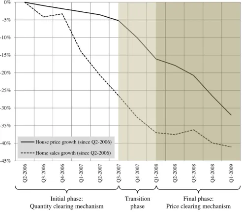
The US housing market crash between 2006 and 2009 challenges the traditional paradigm, as house prices collapsed outright over the course of this crisis, giving rise to a “price clear- ing mechanism”. From peak to trough, the S&P/Case-Shiller National House Price Index plummeted by roughly 32.0% (a later decrease added another 3.8%), which translates into a compound annual growth rate of -13.1%. This was the most violent house price cor- rection ever documented in the US. The eight-year housing recession that extended into the Great Depression saw house prices depreciate by merely 4.4% per year. Even more intriguingly, despite a simultaneous nosedive of 41.0% in home sales, house prices depre- ciated even faster for a large part of the crisis (see Figure 1.1). Only in the early phase
1 The historical house price data stem from Robert Shiller’s website:
www.econ.yale.edu/ shiller/data/Fig2-1.xls. The author uses the Grebler House Price Index and the S&P/Case-Shiller National House Price Index. For details, please consult his seminal work
“Irrational Exuberance” (Shiller, 2009).
2 In a related survey study, Blinder (1982) found evidence of producers of durable goods responding to excess supply by increasing their inventories.
(Q2/2006 to Q3/2007) home sales declined quicker than house prices (26.6% vs. 5.2%).
Following a brief transition phase (Q3/2007 to Q1/2008) when both decreased roughly at the same rate (10.4% vs. 10.9%), house prices growth outpaced home sales (4.4%
vs. 15.9%) in the final phase of the crisis. The paradigm of primarily quantity-driven market clearing is therefore difficult to justify. Instead, the US housing market crash calls for a complementary “price clearing mechanism”.
-45%
-40%
-35%
-30%
-25%
-20%
-15%
-10%
-5%
0%
Q2-2006 Q3-2006 Q4-2006 Q1-2007 Q2-2007 Q3-2007 Q4-2007 Q1-2008 Q2-2008 Q3-2008 Q4-2008 Q1-2009
House price growth (since Q2-2006) Home sales growth (since Q2-2006)
Initial phase:
Quantity clearing mechanism
Final phase:
Price clearing mechanism Transition
phase
Figure 1.1: US house prices and home sales from peak to trough (Q2/2006 to Q1/2009). This figure illustrates the evolution of US house prices and home sales from peak to trough during the recent US housing market crash (Q2/2006 to Q1/2009). In the initial phase of the crisis, home sales decline steeper than house prices. Over the transition phase both depreciate at roughly the same rate. In the final phase of the crisis, the decline in house prices exceeds the one in home sales. Growth rates are computed since inception of the crisis (Q2/2006) based on the S&P Case/Shiller National House Price and existing home sales, respectively. Data sources: Robert Shiller (www.econ.yale.edu/shiller/data/Fig2-1.xls), National Association of Realtors.
This fresh evidence reveals a major gap in the theoretical housing literature. Most existing housing market models fail to account for material price drops. For they are designed in accordance with the “quantity clearing mechanism”. In this reading, homeowners avoid marketing their homes during housing downturns for various reasons. Some models attribute their reluctance to sell to matching issues (cf. Wheaton, 1990; Williams, 1995;
Glower et al., 1998; Albrecht et al., 2007; Chernobai and Hossain, 2012) and others to downpayment constraints (cf. Stein, 1995; Genesove and Mayer, 1997), loss aversion
(Genesove and Mayer, 2001) or anchoring (Bokhari and Geltner, 2011). One notable exception from the mainstream is Qian (2013) who argued in favour of an embedded real option in housing. Another exception is Lazear (2010). The author took the position that homeowners set asking prices strategically to determine the probability of a sale, because they enjoy some monopolistic power. However, all of the above approaches focus a priori on the supply of houses as the predominant factor in the housing market. A theory comprehensive enough to explain material falls in house values or even a reversal of the market clearing mechanism is so far lacking.
In this paper, we therefore develop a novel game-theoretical rationale that features sticky house prices (“quantity clearing mechanism”) during some housing downturns and major price drops (“price clearing mechanism”) during others. The connecting element is the optimal sales strategy of leveraged homeowners. In simplified terms, homeowners possess two options: they either sell immediately at potential fire sale prices or they postpone a sale until their mortgage matures to sit out the negative consequences of the slowdown.3 The best response arguably depends on the severity of the slowdown. Homeowners are inclined to retard a sale under low to moderate excess supply, because the present value of the future sales price plus rent income tends to exceed the immediate short-term house price. However, they lose any interest in delaying a sale strategically once a sufficiently large overhang destroys the home value at maturity. The subsequent uncoordinated sell-off of houses allows prices to plummet in the short term. The model consequently establishes a causal link between the severity of slowdowns, the timing of home sales by homeowners and the way in which housing markets clear.
However, homeowners face a non-trivial decision problem. On one side, they possess some monopolistic power, because housing is durable. They might even postpone a sale for years. This obviously shifts the negotiation power in their favour during market downturns. In fact, their situation is reminiscent of a durable good monopolist, who can freely set the offered quantity.4 On the other side, there are limitations to this strategic behaviour. First, homeowners face external competition as well as rivalling
3 Comparable decision problems relate to the non-participation in labour markets (Murphy and Topel, 1997) or the dynamic pricing of durable goods (Blinder, 1982). Lazear (2010) implicitly pointed in the same direction.
4 In his seminal paper, Coase (1972) conjectures that such a monopolist cannot profit from market power due to time inconsistency. However, extensive research shows ways out of this dilemma, e.g. by monopolizing the after-market, product differentiation or planned obsolescence. For an overview refer to Belleflamme and Peitz (2010).
other incumbents in an oligopolistic fashion. Second, prospective homebuyers, too, gain bargaining power during a market slowdown due to the emergence of excess housing supply. Third, homeowners need to take out a mortgage to finance their initial investment in a similar way to any other capital-intensive durable good. Once their mortgage expires, homeowners are forced to sell (or, equivalently, rollover their mortgage) at the then-house prices. Fourth, homeowners will not postpone a sale, if the short-term house price exceeds the present value of a postponed sale plus rent income. After all, homeowners face a multi-dimensional optimization problem when assessing their best response to a housing downturn.
The presented model examines the optimal sales strategy of homeowners in a framework tailored to accommodate the specifics of housing. The envisioned housing market is segmented. This reflects the market’s heterogeneity across homeowners and regions in reality. Homeowners vary by age, creditworthiness, cultural background, gender, income or marital status. Regions differ by density, infrastructure or macro-economic conditions.
Moreover, homeowners are rational and profit-maximising. They do not suffer a priori from behavioural biases such as loss aversion (Genesove and Mayer, 2001) or anchoring (Bokhari and Geltner, 2011). Homeowners further need to take out a mortgage to finance the initial purchase of a house as houses are highly capital-intensive. Similar financial restrictions are imposed by Stein (1995), Genesove and Mayer (1997) and Brueckner et al. (2011). Finally, the model mimics some of the key characteristics of the US housing market: the market is divided among prime and subprime homeowners, their leverage matches realistic levels, and borrowing is non-recourse (cf. Frame et al., 2008; Harris, 2010, Gao and Li, 2013). The heterogeneous model accordingly portrays various specifics of the housing market.
The simulations of the heterogeneous housing model deliver rich insights. Above all, homeowners may stabilise or compromise house price growth depending on the severity of the slowdown. On one hand, homeowners support short-term house prices by strategically postponing home sales to preserve their medium-term financial interests. The consequent reduction in home sales eventually stabilises the short-term price. On the other hand, as soon as a sufficiently large overhang harms the medium-term financial interests of home- owners their willingness to retard a sale vanishes. This may elicit uncoordinated sell offs spilling over to the competing segment and impairing the short-term house price. Besides,
a segmented housing market is more resilient to low and moderate oversupply, but more vulnerable to substantial overhangs. This is because cross-segment competition provides homeowners with leeway for responding strategically even to segment-specific downturns.
But it also impairs the overall market depth and thus the capacity to absorb substantial overhangs. Hence, the way in which a market clears depends on its fragmentation and on the severity of the crisis: Low to moderate excess supply results in a “quantity clearing mechanism” and a substantial overhang of houses in a “price clearing mechanism”.
Furthermore, a model version accounting for deliberate defaults of homeowners, a lack of available lending volume and other US-specific aspects, well explains several stylised facts of the US housing market crash from 2006 to 2009. The model projections are compatible with the observed house price growth, its negative correlation with foreclosures (Frame et al., 2008), the concentration of foreclosure in the subprime segment (cf. Mian et al., 2009;
Demyanyk and van Hemert, 2011), and the built-up in housing inventory (cf. CoreLogic, 2010; Lazear, 2010). Most notably, both the observed and projected house prices exhibit a
“double drop”—two briefly interrupted consecutive slides. In the model, house price drops occur whenever homeowners deliberately default on their mortgages. The subsequent sell- off of foreclosed homes damages house prices in both segments. Therefore, the negative correlation between house price growth and foreclosures. Besides, subprime homeowners are the first to default since they are particularly leveraged and worst affected by the downturn. This explains the concentration of foreclosures in the subprime segment. The nonetheless material housing inventory is either due to a strategic shortage of prime houses or the inefficient and harmful crowding-out of non-distressed home sales as a result of lacking lending volume. Thus, a model customised to reflect the specifics of the US housing market well explains several stylised facts of the country’s devastating recent housing crisis.
The rest of the paper is organised as follows. Section 1.2 outlines the fundamental game- theoretical idea in a homogeneous setting. This model version is best suited to elucidating the primary dynamics, despite its overly simplistic structure. It also serves as a bench- mark later on. Next, Section 1.3 cultivates the analysis in a more realistic heterogeneous framework. Section 1.4 simulates both model versions and compares the numerical re- sults. Subsequently, we investigate how varying inputs affect the heterogeneous model.
Section 1.5 revisits the recent US housing market crash (2006-2009). We refine the het-
erogeneous model in such a way that it portrays the key characteristics of the country’s housing market at the time: most notably its prime and subprime segments. Finally, we conclude and briefly discuss the policy interventions in the housing market throughout Section 1.6.
1.2 Homogeneous Housing Market
We initially describe the decision problem of homeowners in the least complex setup.
Housing, homeowners and prospective homebuyers are all homogeneous. Later on, hous- ing will become heterogeneous.
1.2.1 Static Equilibrium
Suppose a competitive housing market populated by i∈1, ..., n homogeneous and profit- maximising homeowners, each owning one unit of identical housing worthp. The housing stock is consequently similar to the number of homeowners, h = n. However, since not all houses must necessarily trade on the market, home sales, x≥0, may be smaller than the housing stock, h≥x.
Homeowners invest in housing to realise positive returns over the investment horizon, T, so they need substantial external financing to raise the purchase price (cf. Brueckner et al., 2011). For simplicity, they take on a 100 percent mortgage with a constant interest rate, r, and the same maturity as the investment horizon. Both the principal and the compound interest are due at redemption. The terminal balance due equals p(1 +r)T accordingly. On the other hand, homeowners earn income from their property. For one thing, they realise or save periodical rent, ωp, which is directly proportional to the house price, ω ∈ (0,1).5 By reinvesting the proceeds until maturity, homeowners further accumulate capital gains of I(T) = PT
k=1(1 +r)k so that the capitalised rent income amounts to ωpI(T).6 For another thing, homeowners sell their house at redemption and earnp. Thus, they have funds ofp 1+ωI(T)
at hand to settle their outstanding liabilities
5 This formulation allows me to express that the amount of rent and the house price are typically tied to one another (Gallin, 2008).
6 I(T) follows a geometrical sequence,I(T) =PT
k=1(1 +r)k = [1−(1 +r)T+1]/[1−(1 +r)]>0.
eventually. Equation 1.1 summarises the investment motive:
p 1 +ωI(T)
≥p(1 +r)T. (1.1)
An important corollary is that the fraction of the house price that homeowners periodically extract as rent must never violate ω ≥ (1 +r)T −1
/I(T) to be compatible with the investment motive. In addition, the amount of rent entirely depends on the interest rate and maturity of the mortgage.
Homeowners obtain the needed funding from banks. The banking sector is homogeneous and handles all mortgages. In the tradition of Diamond (1984) and Holmstrom and Tirole (1997), the lending costs comprise the loan volume and monitoring efforts. The aggregate lending volume of the banking sector, lx, is proportional to the individual loan volume, l ≥ 0, and the number of home sales, x. Furthermore, monitoring efforts contain a fixed component,ν > 0, to cover the administrative expenses and a variable transaction-linked component, φ > 0. In economic terms, φ is similar to an agio being paid by borrowers for the service of financial intermediation. The resultant total costs of the banking sector amount tolx+ν+φx, while the marginal lending costs arel+φ. To keep matters simple, the individual loan volume, l, is standardised to one, l= 1.
Prospective homebuyers have the following inverse demand function, which decreases linearly in home sales:
p=α−βx, (1.2)
whereα >0 denotes the reservation price andβ >0 the supply elasticity. In a competitive market, participants have no bargaining power (cf. Belleflamme and Peitz, 2010). The good is supplied at marginal costs,p∗ = 1+φ, and the entire housing stock is for sale,h∗ = x∗. Substituting these two expressions in Equation 1.2 yields the long-run equilibrium housing stock:
h∗ = 1 +α−φ
β . (1.3)
Both the long-run equilibrium house price, p∗ = 1 +φ, and the housing stock, h∗ = (1 + α−φ)/β, play a pivotal role in the subsequent discussion on housing market downturns.
1.2.2 Housing Market Downturns
We define a housing market downturn as a situation of excess supply, i.e. when the existing housing stock exceeds the level that is sustainable in the long run. Since the housing stock barely adjusts in the immediate short term (cf. Case, 2008; Leamer, 2007)—the typical depreciation rate,δ ≥0, is merely about 1.9% (Harding et al., 2007)—even small declines in the demand might drag house prices below their long-run level. On the other hand, homeowners have the option to postpone home sales to a later date, thereby resisting some of the downward pressure. Therefore, how should homeowners respond to housing market downturns and how does their behaviour affect the house price in the immediate short term?
Dates
0 1 2
logical second T
• Market is in long-run equilibrium
• Initial housing stock develops
• Demand declines permanently
• Temporary excess supply of houses
• Homeowners decide on whether to stay in the market or postpone a sale
• Mortgages expire
• Postponing homeowners must sell their houses to redeem their mortgages
• Market may (or not) have completed adjustment to long-run equilibrium
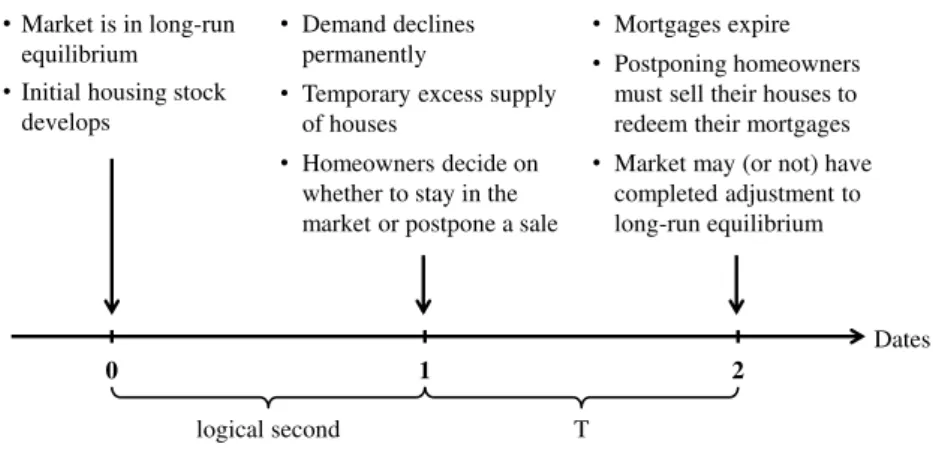
Figure 1.2: Course of events. This figure illustrates how a market downturn evolves in the model.
Time between dates is not equidistant.
In order to characterise the reaction of homeowners to market downturns, we illustrate their decision problem in a dynamic setting (cf. Figure 1.2). The game proceeds on three dates, t = 0,1,2, and the time between them is not equidistant. To distinguish between dates, we add corresponding subscripts to all the time-dependent parameters and variables.
On date 0, the market is in long-run equilibrium. The long-run equilibrium house price accordingly equals p∗0 = 1 +φ with housing stock h∗0 = α0 − (1 + φ)
/β. On date 1, a logical second later, an exogenous shock permanently decreases the homebuyers’
reservation price by ε ∈ (0,1) percent to α1 = α0(1−ε).7 As a consequence, the new
7 The assumption of a permanent decline of housing demand is meant to reflect existing rigidities in housing markets. For instance, even eight years after the start of the US housing crisis demand for
housing stock that is sustainable to the long run reduces to h∗1 = α1−(1 +φ)
/β and creates an oversupply of houses in the amount of ∆h1 = h∗0 −h∗1. This oversupply lasts until continuous depreciation, T δh∗0, eliminates it over time. However, the new long- run equilibrium house price remains unchanged since the marginal costs stay the same, p∗1 = 1 +φ. Short-term home sales, x1, and the house price, p1, are unknown for the time being as the sales decision of homeowners is pending. On date 2, T periods later, all mortgages expire since lenders demand repayment. All homeowners have to sell their properties eventually, independent of the prevalent market conditions. Thus, the entire housing stock is for sale, x2 =h2, and the then-house price equals p2 =α1−βh2. In the best case, all of the earlier excess supply has disappeared, h2 = h∗1. Then, homeowners sell their property without a loss at the long-run equilibrium house price. However, if the housing stock remains elevated, h2 = h∗0(1 −T δ) > h∗1, they will realise a house price below the long-run equilibrium level. The housing stock can be described as h2 = max
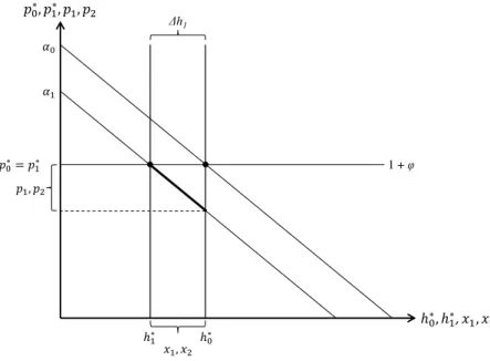
h∗1, h∗0(1−T δ) . Figure 1.3 portrays the market dynamics.
1 + φ Δh1
�∗, �∗, � , �
�
�∗= �∗
� , �
�
ℎ∗ ℎ∗ ℎ∗, ℎ∗, � , �
� , �
Figure 1.3: Housing market dynamics. This figure portrays demand and supply of housing over time. Demand permanently declines. Marginal costs are constant. Housing supply is fixed in the short-term, but elastic in the long-run. Two bold dots define the original and new long-run equilibrium allocations. The bold line denotes the set of potential short-term allocations.
This situation strongly affects the bargain between incumbent homeowners and prospec- tive homebuyers. On one side, the excess supply temporarily frees homeowners from
houses remains below historical levels. Nonetheless, it is noteworthy that the extent of the housing downturn—and thus its impact on the behaviour of homeowners and house prices—would be smaller, if the initial demand shock were to be temporary in nature.
external competition, because building new dwellings is unprofitable as long as the over- supply exists. Therefore, homeowners enjoy some, though limited room for manoeuvre.
Simply put, they either sell immediately at potential fire sale prices, or they postpone a sale until the overhang reduces and the sales prices recover. On the other side, the excess supply lends homebuyers bargaining power to beat down prices, but their bargain- ing power vanishes over time as the oversupply is highest immediately after the demand declines, since the oversupply dissolves over time. Since both homeowners and home- buyers profit to some extend from oversupply the outcome of the bargaining struggle is ambiguous.
To resolve this conundrum, homeowners maximise their individual immediate short-term profits, π1i(p1, x1, c), depending on the house price, p1, home sales, x1, and opportunity costs,c.8 Opportunity costs depend on the benefits and costs of the two strategic options:
selling immediately or postponing a sale. If homeowners sell immediately, they realise the short-term market pricep1 plus first-period rent ωp0. This amounts to (p1+ωp0)(1 +r)T at maturity including compound interest. However, this comes at the cost of foregoing the late market price p2, first-period rent ωp0, and subsequent periodical rent income proportional to the late price, ωp2.9 Including interest earnings this equalsp2(1 +ωI(T − 1)) +ωp0(1 +r)T at redemption. In both cases, homeowners face an identical amount of repayment costs p0(1 + r)T and constant transaction costs λ ≥ 0. Condition 1.4 summarises the trade-off between the two options:
(p1+ωp0)(1 +r)T −p0(1 +r)T −λ
| {z }
capitalised net earnings of immediate sale(t= 1)
≥p2(1 +ωI(T −1)) +ωp0(1 +r)T −p0(1 +r)T −λ.
| {z }
capitalised net earnings of postponed sale (t= 2)
(1.4) Homeowners only sell immediately, if the short-term price outweighs at least the proceeds to be realised until redemption. Otherwise, they postpone a sale. Solving Equation 1.4
8 Departing from typical definitions, costs in this particular context refer to opportunity costs rather than marginal costs, because the latter form sunk costs from a homeowner’s point of view. Home- owners have already bought their house at the original long-run equilibrium house price. These earlier expenses do not affect the pending sales decision of homeowners. What really matters is the present value of a postponed sale which homeowners forego were they to sell immediately.
9 Rent income is proportional top2 so that rent contracts reflect a potentially depressed late price:
p2≤p∗1.
for the short-term pricep1 accordingly returns the opportunity costs of an immediate sale, c= 1
(1 +r)T 1 +ωI(T −1)
p2 ≥0, lim
p2→0c= 0. (1.5)
The opportunity costs equal the present value of the capitalised net proceeds, if home- owners were to postpone their sales.
Meanwhile, short-term home sales x1 depend on external and internal competition, as well as the participation of homeowners. External competition ensures that the house price never exceeds the marginal costs in the immediate short-term. This implies that homeowners cannot drive home sales below the new long-run equilibrium housing stock, x1 ≥h∗1. Otherwise, external investors would seize the profitable opportunity to construct new homes. The bargaining power of homeowners is therefore entirely linked to the oversupply, ∆h1. Internal competition further limits the influence homeowners have on short-term home sales. Let s ∈ (0,1) denote the share of the offered oversupply. Due to the assumed distribution of houses each homeowner controls an equal stake, si, of this share. The remainder, s−i, is commanded by the n−1 competitors: s = si +s−i. So, homeowners have merely humble effect on bargaining power. Also, the participation of homeowners is conditional. For homeowners only participate as long as the house price at maturity is positive, p2 > 0. Otherwise, p2 = 0, they sell anyway, s = 1, because houses neither have a short-term nor a medium-turn value. After all, external (h∗1) and internal competition (∆h1s−i) as well as the conditional participation of homeowners (s) considerably influence short-term home sales, x1 =h∗1+ ∆h1(si+s−i).
This leads us eventually to the optimization problem of homeowners. They maximise their individual short-term profits, πi1 = (p1−c)∆h1si, taking these factors into account:
arg max
s
π1i = α1−βx1 −c
∆h1si s.t. s ∈(0,1),
p2 >0,
wherex1 =h∗1+ ∆h1(si+s−i) denotes short-term home sales. Differentiating with respect to si yields a homeowner’s reaction function:
si = 1 2β∆h1
(1 +φ)−β∆h1s−i−c
. (1.6)
� = ℎ∗+ �ℎ � ��, �−�
� >
Δℎ ≥
Sales strategy.
Type j and k homeowners decide simultaneously.
� = ?
No sales strategy.
Type j homeowners sell immediately.
� =
� = Δℎ ≥
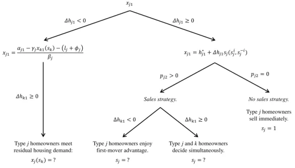
Figure 1.4: Decision problem in a homogeneous housing market. This figure portrays the decision problem of homeowners in a homogeneous housing market in extensive form. Homeowners have an incentive to postpone a sale, as long as houses have an economic value even after retarding a sale, pj2>0. Otherwise, they sell immediately anyway,p2= 0.
By summing for all n individuals, Pn
i si = s and Pn
i s−i = s(n−1), and solving for s, we obtain the Nash-equilibrium share of the offered oversupply, s∗:
s∗ =
n (n+1)
(1+φ)−c
β∆h1 , if p2 >0,
1, if p2 = 0,
(1.7)
provided that s∈(0,1) lies in the defined area.
Equation 1.7 demonstrates that the willingness of individual homeowners to sell their homes in the immediate short term decreases with the size of the oversupply, ∆h1, and opportunity costs, c. Since opportunity costs in turn decline with growing excess supply, the optimal sales strategy of homeowners remains ambiguous after all, which is why we perform simulations at a later stage to ascertain how different levels of excess supply affect home sales and the house price in the immediate short term.
1.3 Heterogeneous Housing Market
We now generalise our analysis to portray a heterogeneous housing market. In the new setting, homeowners and prospective homebuyers are also heterogeneous as they have different preferences for the different types of housing.
1.3.1 Static Equilibrium
There are two heterogeneous types of competitively traded housing. To distinguish be- tween them we add subscript j = 1,2 to all relevant parameters and variables. The housing market is populated by i, ..., n1 type 1 homeowners and i, ..., n2 type 2 homeown- ers. The respective housing stock is hj =nj. Home sales may be lower than the housing stock, xj ≤hj.
As before, homeowners invest in housing to economise on rent,pj 1+ωjI(T)
. They need external financing for the initial purchase of a house. The funding is bullet so that the balance due at maturity is pj(1 +r)T including compound interest. Besides, the funding stems from a homogeneous banking sector serving each type of homeowner a customised mortgage to accommodate their specific capital needs,lj, and monitoring needs,φj. Thus, the marginal lending costs equal lj +φj. Given the market’s competitive nature houses trade at marginal costs, p∗j =lj+φj.
Prospective homebuyers have the following inverse demand which linearly decreases in home sales of both types of housing:
pj =αj −βjxj −γjxk, j 6=k. (1.8)
γj >0 is the supply elasticity concerning the competing type of housing. This way, each housing segment experiences cross-segment competition. The house prices are positively correlated via home sales.10 Thus, even market downturns limited to one housing segment could spread to the other. Since both types of housing are imperfect substitutes the spillover satisfies βj > γj. For γj = 0 homogeneous housing emerges as a special case of Equation 1.8.
Changes in cross-segment competition unwind via home sales. To illustrate this, we re- arrange Equation 1.8 and obtain xj = (αj −pj −γjxk)/βj, j 6= k. By substituting the corresponding symmetric expression of xk into xj, we illustrate homes sales in terms of
10 This assumption reflects that the two types of housing, even though they represent different qualities or regions, are to a large degree similar since they serve the same needs. Thus, they should largely underlie similar economic dynamics.
house prices:
xj = βk αj −pj
−γj αk−pk
βjβk−γjγk
, j 6=k. (1.9)
This formulation demonstrates that an isolated increase in house prices prompts ceteris paribus a substitution effect: If typek housing becomes more expensive (cheaper), typej housing becomes relatively more (less) popular with homebuyers. This is because home salesxjrise (decrease). Therefore, changes in cross-segment competition dissipate through home sales.
Furthermore, Equation 1.8 allows us to characterise the long-run housing stock. Since both types of housing are traded competitively, houses are supplied at marginal costs, p∗j =lj+φj, with the entire housing stock being up for sale, x∗j =h∗j. Thus, the long-run equilibrium housing stock is: h∗j = βk(αj−(lj+φj))−γj(αk−(lk+φk))
/(βjβk−γjγk),j 6= k. Notice that the new long-run housing stock is always smaller than in the homogeneous case. To see this, imagine that the difference in parameters vanishes (i.e. subscripts disappear) and the loan volume is again standardised to l = 1. Then, the long-run housing stock simplifies to h∗j = (β−γ)(α−(1 +φ)
/(β2−γ2). Thus, the present and previous housing stock merely differ in terms of (β −γ)/(β2 −γ2) ≶ 1/β. Since β > γ, it follows that β(β −γ)/(β2−γ2) < 1. Hence, 1/β > (β−γ)/(β2 −γ2). The intuitive reason for this finding is that heterogeneity interferes with competition since spillovers are imperfect (βj > γj). Accordingly, the home sales are higher when we abstract from heterogeneity.
1.3.2 Housing Market Downturns
In a heterogeneous setting, a market downturn denotes a situation of excess supply in at least one housing segment. The affected homeowners must decide whether to exploit the durability of housing and postpone a sale or not.
Again, there are three dates, t= 0,1,2, and the dates are not equidistant. To distinguish the dates, we add another subscript to all time-dependent parameters and variables.
The housing downturn evolves in the same way as before. On date 0, the market is in long-run equilibrium. The house prices and home sales accordingly equal their static equivalents: p∗j0 =lj+φj andh∗j0 = βk(αj0−(lj+φj))−γj(αk0−(lk+φk))
/(βjβk−γjγk),
j 6=k. On date 1, a logical second later, the demand for houses declines permanently. To emphasise the heterogeneity of the housing market, the drop in reservation pricesε ∈(0,1) may affect each segment differently depending on the shock co-movement ρ ∈ (0,1).11 The new reservation prices are αj1 =αj0(1−ε) for type j houses and αk1 =αk0(1−ρε) for type k houses. Type j housing is therefore worst affected by the slowdown. The new long-run equilibrium house prices and home sales become p∗j1 = lj +φj and h∗j1 =
βk(αj1−(lj+φj))−γj(αk1−(lk+φk))
/(βjβk−γjγk),j 6=k. Short-term home sales,xj1, and house prices,pj1, are unknown for the time being as the sales decision of homeowners is pending. On date 2, T periods later, all outstanding mortgages expire thereby compelling homeowners to sell their houses. Thus, home sales match the housing stock, xj2 = hj2. The resultant house prices are pj2 =αj1 −βjhj2−γjhk2.
However, a housing downturn may unwind very different from before due to cross-segment competition. The latter interferes with the initial size and direction of excess supply, the depreciation dynamics and how homeowners maximise their profits. First of all, a down- turn provokes an overhang only in the worst-hit housing segment while the other might even witness a lack of houses because of the cross-segment substitution effect described earlier. If a negative demand shock makes a certain housing segment less attractive, the other becomes ceteris paribus more popular. Therefore, only the worst-hit housing seg- ment suffers excess supply in any event, ∆j1 ≥ 0.12 What happens to the competing segment k is ambiguous, since the latter is potentially less affected by the demand shock.
Typek housing only witnesses an oversupply, ∆k1 ≥0, if the shock co-movement is both positive and outweighs the cross-segment substitution effect,ρ≥γkαj0/βjαk0 >0.13 Oth- erwise, the segment lacks houses, ∆h21 < 0. Hence, only the worst-hit type of housing faces an oversupply with certainty during a housing downturn, whereas the other segment may even lack houses.
Second, the cross-segment competition may complicate the depreciation dynamics de- pending on the initial excess supply. For one thing, if a given segment still suffers a surplus of houses at maturity, ∆hj1 ≥ T δh∗j1 ≥ 0, the housing stock in the other seg- ment may equilibrate the aggregate housing market, by temporarily depreciating below
11 We limit the correlation to non-negative values in order to ensure that any housing downturn has at least a tendency to negatively affect the housing market in general.
12 Under the given assumptions, h∗j0, h∗j1 ≥ 0 and αj0 ≥ αj1. Hence, h∗j0 ≥ h∗j1, so that ∆hj1 ≥ 0 follows independent of the shock co-movement.
13 Rewriting the respective excess supply gives ∆k1=ε(βjαk0ρ−γkαj0)/(βjβk−γjγk)≥0. Solving the expression forρreturns the condition.