Liquidity and prices: A cluster analysis of the German residential real estate market

(1)

O R I G I N A L P A P E R

Liquidity and prices: A cluster analysis of the German residential real estate market

Marcelo Cajias

¹

· Philipp Freudenreich

²

· Anna Freudenreich

²

· Wolfgang Schäfers

²

Published online: 16 August 2020

Abstract

This paper analyses the highly under-researched German residential real estate mar- ket. Quality- and spatial-adjusted price and liquidity indices are calculated separately for the investment and rental market on a regional basis. Applying the “Partitioning Around Medoids (PAM)” clustering algorithm, the regions are clustered with respect to their price and liquidity development after the average silhouette method is applied to find the optimal number of clusters. The dataset underlying this analysis com- prises more than 4.5 million observations in 380 German regions from 2013 Q1 to 2018 Q4. The clusters are then analysed by means of further economic and socioeco- nomic data in order to identify similarities. Furthermore, the clusters are interpreted from a geographic perspective. We find that the allocation to cluster 1 is always sup- ported by higher growth rates in the variables, population, working population and real GDP, implying higher demand for space. Moreover, in each of the analysed cat- egories cluster 1 reveals a lower unemployment rate as well as a higher disposable income. One of the most interesting implications is, that apparently a large part of the German population has developed into professional real estate investors. In Germany the largest share of landlords is the one of the so-called non-professional landlords. As the regions assigned to cluster 1, displaying the most significant price increase, seem to be chosen based on a very sophisticated market analysis by identifying the regions with the strongest fundamental data, it seems like the dominating market players have significantly increased their knowledge and approach for investing in residential real estate.

Keywords Residential · Housing · Liquidity · Index · Time on market · GAMLSS · Cluster · Partitioning around medoids

JEL Classification R2 · R21 · R3 · R32

The online version of this article (https://doi.org/10.1007/s11573-020-00990-2) contains supplementary material, which is available to authorized users.

Extended author information available on the last page of the article

(2)

1 Introduction

Financial assets such as stocks and bonds are traded in tremendous volumes, turning over billions of dollars within seconds and with almost no spatial constraints. By contrast, the transaction process of direct real estate is more complex, often consuming several months due to the heterogeneity of individual properties and market specific frictions. For example, larger participation-, search- and transaction-costs, as well as considerable asymmetric information impede a smooth match between buyer’s or tenant’s and seller’s or landlord’s price expectation within “short” time intervals.

When it comes to residential real estate—an asset class which is strongly linked to individual preferences of buyers and tenants as well as expectations of sellers and landlords—a matching of both sides may be even more difficult. Thereby, the location of the respective dwelling plays a major role for the development of the key features determining the matching process.

On the residential real estate market, the process of selling or renting out a dwelling comprises of two essential components. The first component is the introduction of the dwelling onto the market at a price

¹

determined by the seller or landlord. The second component is the time it takes until a prospective buyer or tenant is willing to take the dwelling off the market and to pay the price.

²

Contingent upon a matching of the expectations of supply and demand, a market is able to operate. The easier, thus faster this matching occurs, the higher the liquidity on the market. Liquidity is related to price in both cause and effect. According to Geltner et al. (2014), increased market activity, displayed by a higher number of transactions as well as a rising transaction frequency on the residential market, leads to more similar properties in the respective market. Hence, the observation of relevant transaction prices becomes easier. As the information of properties being transacted in the relevant market directly influences the individuals’ price assessment of other properties, potential market participants become better informed, leading to less market uncertainty. Thus, potential buyers or tenants and sellers or landlords can form improved reservation prices, so that the respective distributions become narrower and converge to the “equilibrium price”.

³

Consequently, transaction prices improve and so does liquidity. In the following, liq- uidity is defined as the inverse of the time on market (TOM). Typically, the matching will occur faster if the price of the dwelling is supported by its particular location and building characteristics. Depending on the level of demand, buyers and tenants might start to accept higher prices. But as long as there is sufficient supply, the prospective buyer or tenant will continue to search the market and not rush into an undesired con- tractual agreement. Therefore, the buyer or tenant is said to be the provider of liquidity, as he has the financial resources to afford the dwelling and to convert it into cash or a

1 In the following, the term “price” refers to the price on the investment as well as the rental market and is distinguished as “price on the investment market” and “price on the rental market”.

2 Due to a lack of transaction prices and contract rents on the German residential market the asking price and asking rent, respectively, operate as a “take it or leave it option” to the buyer or tenant and thus price negotiations are not considered as well (see Sect.3).

3 The “equilibrium price” is defined as the price, where the market clears, leading to maximum transaction volume and maximum liquidity. This is the case, when there is no asset price uncertainty and all potential market participants are perfectly informed.

(3)

dividend yielding asset for the owner or landlord, see Fisher et al. (2003). Only if it is up to “take what you can get”, buyers and tenants will be accepting a price which is exceeding their initial reservation price in no time.

Currently, the assessment of the real estate market is mainly based on the consid- eration of prices. Hence, the price development is captured by a variety of indices worldwide, see European Central Bank (ECB), Bank of International Settlements (BIS) and International Monetary Fund (IMF), among others, to assess the state of the residential market. However, not including information about the time it takes to sell or rent out a dwelling might lead to an incorrect assessment of market phases or spatial markets, respectively. To improve the assessment of the residential market, this paper additionally provides quality- and spatial-adjusted liquidity indices for the residential investment and rental market, as complementary demand indices. Hence, this paper aims to provide deeper insights to the under-researched German residential real estate market by combining the consideration of price and liquidity indices. Both indices are developed for the investment and rental market separately for 380 of 401 NUTS 3 regions. The approach is based on the matching of three data sources on an applied big data environment with more than 4.5 million observations, split into about 1.5 million on the investment market and about 3 million on the rental market.

Over the last decade, Germany has experienced a strong and enduring economic expansion. The fundamental economic data exhibits a growing GDP, accompanied by historically high levels of labor demand. The consistently favorable macroeconomic situation and geopolitical events triggered high migration from within the European Union as well as from outside. In addition, the number of households has been increas- ing due to the social trend towards fewer household members. Furthermore, interest rates for mortgages have been extremely low, resulting in higher affordability of homeownership. Unsurprisingly, this economic and socioeconomic development led to booming demand for residential real estate. Despite rising building permissions and construction activity, building completions have been insufficient to meet demand in many regions. In a study of the Federal Institute for Research on Building, Urban Affairs and Spatial Development (BBSR), Held and Waltersbacher (2015) identified an increased demand of 272 thousand new dwellings per year for the years 2015–2020.

The statistics of the Federal Statistical Office (2019a) show that not in a single year since the BBSR published the study, enough new dwellings entered the market (max.

251 thousand in 2018). As consequence, vacancy rates fell below sustainable levels in many regions and house prices as well as rents have experienced upside pressure. The official national house price index of the Federal Statistical Office (2019b) reveals a national price increase of 36% for the last 6 years. According to the big data sample used for this study, which includes about 1.5 million observations on the investment market, asking prices increased by 44% on average within the same period.

⁴

A decom- position of the consumer price index published by the Federal Statistical Office (2019c) reveals an increase in rents of a mere 9.6% for the last 6 years. Again, the current big

4 The difference to the Federal Statistical Office might be caused due to the fact that this paper only covers 380 regions in the sample in order to avoid a bias stemming from inactive markets. The Federal Statistical Office, however, includes all regions, and thus the inactive markets that mostly show relatively weak price developments drag the average price development down. Hence, the Federal Statistical Office exhibits a slightly lower price increase compared to our results.

(4)

data sample of more than 3 million rental offers reveals an increase of 14.9% within the same period.

The price appreciation on the rental market seems innocuous in comparison to the one experienced on the investment market. With a homeownership rate of 43% as of 2013,

⁵

the first year covered by the current sample, more than half of the German population rent their homes. While Voigtländer (2009), among others, discussed in detail the reasons for the extraordinarily low homeownership rate, research on the nationwide rental market is rather scarce. Furthermore, the ratio of observations on the rental market to observations on the investment market in this paper is about 2:1 and hence demonstrates the importance of the rental market in Germany. Simply based on the moderate appreciation in asking rents, it is hardly possible to make any inferences with regard to a tight rental market. Are the stories about property viewings with more than 50 competitors for the same flat only urban myths? Maybe the analysis of the liquidity on both residential markets reveals the somehow hidden demand. By only looking at the average change in time on market, it seems as there is only a rather small difference between the investment and the rental market, as the liquidity improved by 50% and 39.5% respectively. An estimation of quality- and spatial-adjusted liquidity indices, however, exposes the real difference in market tightness.

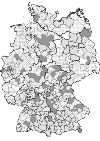
However, the price and liquidity development are geographically not equally dis- tributed across the country. A booming trend is mainly observed in the major cities, their surrounding conurbations as well as economically strong regions in southern and north-western parts of Germany. In contrast, rural regions in the east of the country as well as structurally weak regions in the western parts are left behind. Consequently, these areas suffer from the ongoing urbanization and the concomitant rural emigra- tion, leading to low demand and high vacancy rates. Hence, the price and liquidity development differ significantly within Germany. Therefore, it is not sufficient to con- sider the German market as a whole but to split it up into a regional analysis. That is why, a cluster analysis is conducted in this paper in order to detect economic and socioeconomic similarities and differences of flourishing and fading regions.

The study aims to answer the following questions regarding the residential real estate market.

1. How did price and liquidity on the German residential investment and rental market measured by quality- and spatial-adjusted hedonic indices evolve over the last 6 years?

2. To what extent can the markets be clustered? What similarities and differ- ences in view of economic and socioeconomic indicators do these regions share?

3. Which overall conclusions and implications can be drawn for the German residential real estate market?

The remainder of this paper proceeds as follows: The next section reviews the cur- rent state of the literature. Section 3 describes the dataset and the descriptive statistics.

Section 4 presents the econometric model, including the derivation of the hedonic

5 According to GdW (2016).

(5)

price and liquidity indices as well as the clustering algorithm. Estimation results are presented and discussed in Sect. 5. Section 6 concludes.

2 Literature

As mentioned above, a deeper understanding of the residential real estate market can only be achieved by examining the price development in combination with the liquid- ity development. Generally, several liquidity proxies exist for the real estate markets.

In line with Sarr and Lybek (2002), Ametefe et al. (2011) summarize various liquidity indicators into five main categories: (1) transaction cost measures, (2) volume-based measures, (3) price impact measures, (4) return-based measures and (5) time-based measures. (1) Transaction cost measures are mainly used for the liquidity analysis on the financial market, see e.g. Clayton and MacKinnon (2000). A market is described as liquid when transaction costs are relatively low. Liquidity is commonly approximated by the spread between the bid and ask price, empirically going back to Demsetz (1968), and related measures. The smaller the spread the more liquid the market. Hence, the bid-ask spread is a measure for market liquidity as well as a transaction cost measure.

According to Geltner et al. (2014) the bid price would equal to the asking price, hence,

“equilibrium prices” would be charged implying market clearing, if there was a fric- tionless market with all market participants being perfectly informed about property values. However, when it comes to residential real estate—an asset class which is strongly linked to individual preferences of homebuyers or tenants and expectations of home-sellers or landlords as well as to asymmetric information—both counterpar- ties reveal a different valuation for the same asset. As long as transaction markets are considerably active, both market participants can observe various transaction prices of similar properties. Consequently, they build their beliefs about prices as a distribution around the likely “equilibrium price”. Hence, the higher the transaction frequency on the respective market, the closer the spread between the bid price and the asking price, and in turn the higher the liquidity on the market. To apply this liquidity measure to the German residential real estate market, however, is not possible in this paper due to data restrictions regarding bid prices. (2) Volume-based measures depict liquidity as the absolute or relative number of transactions. It is mainly used for the liquidity analysis of listed real estate, see e.g. Brounen et al. (2009), however, e.g. Fisher et al. (2009) apply it on the direct real estate market as well. Volume-based measures comprise the transaction volume, the turnover ratio, the quote size, the number of bids and the market depth. The transaction volume is a very popular measure of liquidity in the literature due to its simplicity and data availability. The transaction volume in a specific period is calculated as the sum over all traded assets (price times quantity of an individual asset) in a specific period. Following Geltner et al. (2014), from a theoretical point of view a higher trading volume implies that the assets are generally more similar and, hence, the information of transactions has a greater impact on the appraisal of other assets.

Consequently, the distributions of the reservation price of buyers and sellers are con-

verging, decreasing the bid-ask spread as well as the transaction costs and, thus, leading

to higher liquidity. Another commonly used liquidity measure is the turnover ratio,

however, due to its calculation (transaction volume divided by the product of existing

(6)

stock and price) is not popular for the direct real estate market as these variables are harder to estimate as e.g. for the stock market. (3) Furthermore, there are different liq- uidity proxies belonging to the group of price impact measures. These proxies have in common to measure liquidity by separating liquidity from other factors that influence real estate prices. The Amihud (2002) measure for example, applied by Karolyi et al.

(2012) as well as Glascock and Lu-Andrews (2013) for instance, is commonly used in the finance literature. Another proxy would be the Pastor and Stambaugh (2003) liquidity factor which is a monthly liquidity measure based on daily data that refers to occasional price changes. (4) Return-based liquidity measures have the advantage that the calculation requires no further information besides the price indices. These mea- sures include for example the illiquidity proxy, developed by Das and Hanouna (2010), which calculates the run length of returns. (5) The liquidity measure used in this paper belongs to the time-based measures. They contain the holding period and the trading frequency, measuring liquidity as the frequency an asset is traded. The holding period, for example applied by Amihud and Mendelson (1986), is empirically applied as the inverse of the turnover rate. For a better suited application in financial markets this liquidity measure was corrected for untraded assets by Collett et al. (2003). Another popular time-based measure is the time on market, measuring liquidity as the time it takes to transact a certain asset. The time on market is especially used in the direct real estate market and is addressed in Krainer (1999) and Allen et al. (2009) among others. The time on market is the measure used in the underlying paper.

As most other markets, the residential real estate market exhibits cyclical move- ments over time. According to the seminal work of Kluger and Miller (1990) who developed a liquidity measure by using the Cox (1972) proportional hazards model, housing prices and liquidity exhibit a positive correlation. Thus, prices and liquidity should match along “hot” and “cold” market states. Krainer (1999) defines a market as “hot” when prices are increasing, the time on market is short and transaction vol- ume is above average. In contrast, decreasing prices, relatively long selling times and low transaction volumes point to a “cold” housing market. A positive correlation is found in Berkovec and Goodman Jr. (1996) for instance. Follain and Velz (1995) for example, find a negative correlation. While Stein (1995) and Genesove and Mayer (1997) reason the correlation with sellers’ equity constraints, i.e. with frictions on the credit market, Krainer (1999) shows that “hot” and “cold” real estate markets emerge due to search frictions and asymmetric information. Cauley and Pavlov (2002) show evidence for the option value of homeowners and for nominal loss aversion. Substan- tial deviations from these two market states might indicate speculative expectations by investors and landlords, adjustment processes or supply and demand changes. To detect these deviations is essential for real estate market participants, as it is otherwise impossible to reduce the risk in investment decisions.

Literature in the price-liquidity field focuses predominantly on the US residential investment market. At the same time, academic research concerning real estate market movements on the German market is rather scarce. While most of the literature strand focuses on “hot” and “cold” market phases along the residential cycle, this paper aims to detect “hot” and “cold” market spots on a regional basis. As one of the few papers on the German market, an de Meulen and Mitze (2014) identify “hot” and “cold”

spots on the Berlin residential market. In order to detect those, the authors exclusively

(7)

investigated the price aspect of dwellings. In general, the movements on the residential real estate market are described primarily with price indices. On the overall German market, there are hedonic price indices provided by the Federal Statistical Office as well as indices provided by private companies like e.g. bulwiengesa

⁶

and Immobilien- scout24 (IMX). The methodology and data behind the IMX are described in Bauer et al. (2013). However, a complementary liquidity index and a combination between both are missing. As mentioned above, it is precisely needed to look simultaneously at prices and liquidity when understanding the current and future state of residential real estate markets. Especially for central banks, policy makers, institutional investors, and private households it is essential to be aware of the liquidity momentum, as both indices might move in opposite directions, pointing to different market states. Thus, solely considering the price index for classifying a regional market might lead to incorrect investment strategies and policy implications. Therefore, this paper devel- ops a quality- and spatial-adjusted price and a complementary liquidity indicator for the investment and rental market of 380 German regions. According to the indices, the regional housing markets are then clustered in order to reassess the assumption that prices and liquidity move together or whether their dynamic behavior exhibits fric- tions. For more than 25 years, bulwiengesa has been providing a clustering of German cities according to their size, measured by the number of inhabitants, the size of the office market and the importance of the city for the national as well as international real estate market. Heinrich and Just (2016) have noted, that those characteristics might not be entirely sufficient for concluding that housing markets form a cluster. While the approach of Heinrich and Just (2016) and the one presented in this paper both use clustering methods, the latter one does not directly cluster a variety of variables directly but uses them for the preceding empirical index calculation. In addition to the quality- and spatial-adjusted regional price indices, a liquidity index for each mar- ket, respectively, is introduced as an additional clustering indicator. The indexing and clustering on a regional level yields a very granular analysis of the German residential investment and rental market and allows the identification of “hot” and “cold” spots.

The findings should be of interest to households, institutional investors and policy makers trying to steer the residential market.

3 Data and descriptive statistics

In the underlying paper data is gathered from four data sources. Real estate data, including prices on the investment and rental market, are taken from empirica systems (https://www.empirica-systeme.de), which collects georeferenced real estate data from more than 100 German Multiple Listing Systems (MLS) such as the market leaders ImmoScout, Immonet or Immowelt but also regionally focused market places and newspapers for the whole German market. As the market leader of real estate data for Germany, empirica has an own proprietary algorithm that identifies doubles and harmonises the sample. Furthermore, the number of households and the purchasing

6 bulwiengesa is one of the largest independent consulting companies on the real estate market in continental Europe.

(8)

power per household on a ZIP basis are obtained from the “Gesellschaft für Konsum- forschung” (GfK) for 2017. The geo-shapefiles of the German territory are extracted from Eurostat in order to calculate two spatial gravity variables: the distance to the centroid of the NUTS 3 region and to the ZIP-centroid. Although the ZIP regions are all part of the larger NUTS 3 regions, the correlation of the variables used for this approach is only 0.311 on the investment market and 0.322 on the rental market.

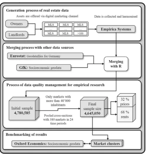
After merging the data and calculating the gravity variables, we proceed with the data selection. This paper only focuses on active residential real estate markets with more than 100 observations and more than 40 thousand inhabitants in order to avoid a bias stemming from a lack of observations on the respective market and outliers. Thus, the number of considered NUTS 3 regions is reduced from 401 to 380 as well as the initial sample size of 4,780,585 observations is reduced to 4,645,050 observations. In total, 1,476,592 observations on the investment market (prices) and 3,168,458 observations on the rental market (rents) in 380 German regions from the first quarter of 2013 to the fourth quarter of 2018 are applied for the estimations. Economic and socioeconomic data for the NUTS 3 regions is gathered from Oxford Economics and is used for the explanation and interpretation of estimation results. The data generating process is depicted in Fig. 1.

This paper exclusively uses asking prices and asking rents. Due to a lack of trans- action prices and contract rents on the German residential market the asking price and asking rent, respectively, operate as a “take it or leave it option” to the buyer or tenant and thus price negotiations are not considered as well. On the residential rental market this assumption is plausible as negotiations about the monthly rental payments are rather an exception. Regarding the property market, Shimizu et al. (2012) com- pare different house prices—asking prices, contract prices and registry prices—on the Japanese housing market. They conclude that for the different house prices and, thus, different datasets there exist differences in the housing price distribution, which can be traced back to quality differences. However, after controlling for quality differences across the datasets no substantial differences between the house price distributions are to observe. Another peculiarity of this study is the application of the total price in Euro of a dwelling offered on the investment market and the total monthly rent in Euro for a dwelling offered on the rental market, although the more popular approach is the utilization of price and rent per square meter. When estimating time on market, we observed that the application of those commonly used variables yields economically incomprehensible relationships for the impact of changes in price (improves liquidity all else equal) and living area (decreases liquidity all else equal) on liquidity. The time on market, is defined as a non-negative continuous variable, measuring the time elapse that a dwelling requires to change its status from being offered on the market to being out of the market in weeks calculated by its start and end date. Typical housing attributes included in this study are hedonic characteristics like “living area”, “age”

and “number of rooms” as well as binary hedonic characteristics like for example

“with balcony”, “with parking slot”, “with elevator”. Since the data is georeferenced,

NUTS 3 regions have been employed as geographical analysis units and are defined

by Eurostat to the “Nomenclature of Territorial Units for Statistics”, which is a hierar-

chical system for dividing the economic territory in Europe. Hence, this classification

provides the possibility of statistical comparison of regions within the EU. NUTS 3

(9)

Fig. 1Generation process of residential real estate data

regions are the smallest classification units, thus cover small regions that are related to

counties or administrative districts. This classification of spatial territory is strongly

related to the administrative division of the country. Subsidies for specific regions are

also assigned according to the classification of NUTS regions. Michels et al. (2011)

criticize that this type of classification exhibits the administrative structures, however,

cannot depict economic and functional linkages to the surrounding areas. They pro-

pose to classify the regional markets into “housing market areas”, defined as areas

where a household lives and works and within that area the household will search

for an alternative place to live in the case of relocation. Hence, Michels et al. (2011)

take migration as well as commuting flows into account and make their classification

more functional. Even though the classification into “housing market areas” consti-

tutes a very effective approach, it is not applicable to the underlying paper. The aim

of this paper is to allocate regions to clusters according to their price and liquidity

development and further to detect economic and socioeconomic similarities of these

(10)

regions. Consequently, an official classification is inevitable in order to match the clus- tered regions to economic and socioeconomic data based on the same regional level.

Furthermore, the classification of “housing market areas” might lead to a different classification on the investment and regional market. Hence, this could lead to further complications regarding the underlying paper.

The variables, their units and sources can be found in Table 1.

Figure 2 shows the cumulative mean price and time on market development on the investment (IM) and rental market (RM) from the first quarter of 2013 until the end of the observation period. It is visible that prices have been increasing accompanied by a diminishing time on market on both markets. Hence, both indicators point to a boom phase on the German housing market, triggered by ongoing demand with supply lagging behind. Moreover, it is observable that prices on the transaction market have been increasing considerably more than rents. While rents have been rising by a mere 14.9%, prices on the transaction market have experienced a substantial growth of 44% over the last 6 years. Those figures indicate a particularly high demand on the investment market, probably triggered by constantly low mortgage rates on housing loans and a lack of interest-bearing investment opportunities.

It seems that the price development has not yet been fully absorbed by the rental mar- ket. The relatively moderate growth in rents seems to only reflect the natural demand, which obviously was higher in cities. As landlords will try to pass on the rising prices on the investment market to their tenants, it might indicate further rental growth in the near future. Of course, rental protection laws prohibit landlords to hand over the entire increase in transaction prices to tenants in order to meet their target return. Asking exorbitant rents has been prohibited on the German market for years, not only since the introduction of rent control in 2015. Because of lacking investment alternatives, new landlords somehow became acquainted to shrinking rental yields. Nevertheless, time on market exhibits an enormous decrease of about 50% on the transaction market and about 40% on the rental market with an almost parallel development on both markets.

Although prices on the investment and rental market have not experienced growth of equal magnitude, the similar development of time on market indicates consider- ably high demand on the rental market, which might also result in upward pressure on rents. To reason the similar drop in time on market with relatively more supply on the rental market in relation to the investment market is rather less plausible, as newly built dwellings are usually offered on the investment market, before they appear on the rental market. Thus, this slightly controversial finding emphasizes the impor- tance of focusing on both indicators—price and time on market—when analysing the residential real estate market.

Figure 3 exhibits, that heterogeneity is omnipresent on the housing market. Panel A to D show, that households within different purchasing power percentiles demand a different price, living area, and distance to the city center. Furthermore, it is shown that the sales and letting process with respect to the marketing time varies.

Generally, relatively richer households can afford more expensive dwellings, pre-

fer larger living areas, tend to live further away from the city center and spend less

time on the search and matching process. These preferences are visible for the invest-

ment as well as the rental market. Surprisingly, buyers living within zip codes with

very low purchasing power (20th-, 30th percentile) pay on average higher prices than

(11)

Table1Variablesandsources VariableUnitEffectintheestimationequationsSources HedoniceffectsSpatialeffectsSocioeconomiceffectsEmpiricaGfKEurostat Askingpricee✓ Askingrentepermonth✓✓ TimeonmarketWeeks✓✓ Livingaream2✓✓ AgeYears✓✓ RoomsNumber✓✓ WithbathtubBinary✓✓ Withbuilt-inkitchenBinary✓✓ WithcarspaceBinary✓✓ WithterraceBinary✓✓ WithbalconyBinary✓✓ WithelevatorBinary✓✓ NewlybuiltdwellingBinary✓✓ RefurbisheddwellingBinary✓✓ GaussianlongitudeCoordinate✓✓ GaussianlatitudeCoordinate✓✓ DistancetoZIPcentroidkm✓✓ DistancetoNUTS3centroidkm✓✓ HouseholdsinZIPHHs/ZIP✓✓ PurchasingpowerofHHsinZIPe/HH/p.a./ZIP✓✓ N4,645,050

(12)

-10 0 10 20 30 40 50

2013Q1 2013Q2 2013Q3 2013Q4 2014Q1 2014Q2 2014Q3 2014Q4 2015Q1 2015Q2 2015Q3 2015Q4 2016Q1 2016Q2 2016Q3 2016Q4 2017Q1 2017Q2 2017Q3 2017Q4 2018Q1 2018Q2 2018Q3 2018Q4

Panel A: Cumulative percentage change in mean price, investment and rental market

Δ price, IM Δ price, RM

-80 -70 -60 -50 -40 -30 -20 -10 0 10 20

2013Q1 2013Q2 2013Q3 2013Q4 2014Q1 2014Q2 2014Q3 2014Q4 2015Q1 2015Q2 2015Q3 2015Q4 2016Q1 2016Q2 2016Q3 2016Q4 2017Q1 2017Q2 2017Q3 2017Q4 2018Q1 2018Q2 2018Q3 2018Q4

Panel B: Cumulative percentage change in mean time on market, investment and rental market

Δ time on market, IM Δ time on market, RM

Fig. 2Cumulative percentage change in mean price and mean time on market. This figure plots the cumulative percentage change in mean price on the residential investment and rental market as well as the cumulative percentage change in time on market on the residential investment and rental market. The data consists of 1,476,592 observations on the residential investment market and 3,168,458 observations on the residential rental market. The sample period is 2013 Q1 to 2018 Q4

the middle-income (40th-, 50th-, 60th percentile) groups. On the investment market

a reason for that might be that the living area demanded by households at the 40th

and 50th purchasing power percentile is lower than at the 30th percentile and further-

more, these households live further away from the city center. However, this cannot

(13)

13 14 15 16 17

2,00,000 2,50,000 3,00,000 3,50,000 4,00,000

10th 20th 30th 40th 50th 60th 70th 80th 90th 100th

Panel A: Price (in €, left y-axis) and time on market (in weeks, right y-axis), investment

market

price time on market

5 6 7 8 9 10

79 81 83 85 87 89

Panel B: Living area (in m², left y-axis) and distance to NUTS 3 center (in km, right y-

axis), investment market

living area distance to NUTS 3 center

5 6 7 8 9 10 11 12

400 500 600 700 800

Panel C: Price (in €, left y-axis) and time on market (in weeks, right y-axis), rental

market

price time on market

5 6 7 8 9 10

60 66 72 78 84

Panel D: Living area (in m², left y-axis) and distance to NUTS 3 center (in km, right y-

axis), rental market

living area distance to NUTS 3 center Fig. 3Distribution of selected variables across purchasing power percentiles. The figures plot the distribution of selected variables segmentd by purchasing power percentiles. The data consists of 1,476,592 observations on the residential investment market and 3,168,458 observations on the residential rental market. The sample period is 2013 Q1–2018 Q4

be observed on the rental market. Another interesting fact is, that the range between

the highest and lowest income group with respect to prices, living area and time on

market is remarkably more pronounced on the rental market relative to the investment

market. While on the investment market asking prices, living area and the time on

market between the richest and poorest percentile vary by 68.7%, 10.2% and 17.8%,

the differences on the rental market are much stronger with 85.3%, 27.7% and 50.1%,

respectively. This infers that the participants and probably also the dwellings on the

rental market are much more diversified than those on the investment market. It seems

surprising, that relatively rich households tend to spend much more on renting than

on the investment in a dwelling compared to relatively poor households. Regarding

the distance to the city center it is noticeable that especially among the poorest, an

increase in purchasing power leads to a very strong shift of investments further away

from the city center.

(14)

4 Econometric approach

The aim of a price index is to measure the price development over successive peri- ods after correcting for hedonic characteristics. However, residential dwellings are not transacted periodically, but rather irregularly and even infrequently. Furthermore, residential real estate is extremely heterogeneous, both in terms of its physical char- acteristics and its location. Dwellings with different characteristics and in different locations might exhibit distinct price and liquidity dynamics in terms of volatility and cyclicality. Thus, idiosyncratic price and liquidity movements might be to observe in diverse markets, due to social, and economic circumstances in a particular region. In order to control for heterogeneity, hedonic indexing is applied in this paper. The hedo- nic approach is a method for generally indexing economic prices of goods affected by quality changes. Kain and Quigley (1970) were among the first to apply hedonic pricing to the real estate market. Given hedonic data, the hedonic model decomposes the price as well as the liquidity of residential real estate into individual character- istics. Hence, the computed index reveals constant characteristics and consequently points out the pure price and liquidity changes over time. The location of a dwelling is probably one of the most important determinants of prices and liquidity. Therefore, not only postcode identifiers as well as longitude and latitude data are considered in the functional form, but the price and liquidity indices are estimated individually for each market p ∈ {1,…,380}, defined by the NUTS 3 regions. In this paper, the time-dummy method is applied, which is defined as the marginal change in price (liquidity) with respect to time. Thus, a transformation of the estimated coefficients of the time fixed effects yields the price (liquidity) index, referring to the percent- age marginal change in prices (liquidity) in period t

t

relative to period t

0

. Hence, the indices can be computed directly from the estimated coefficients. Compared to the imputed hedonic index no “representative dwelling” must be defined and it is less data intensive and therefore very well suited for the construction of regional price and liquidity indices. The standard model for the estimation of a time-dummy hedonic index is given as

y = X β + μθ + u . (1)

As the semi-log functional form has proven appropriate and is used in most hedonic regression models according to Halvorsen and Pollakowski (1981) as well as Diew- ert (2003), among others, y is an i-vector consisting of the elements y

i

= ln(p

i

).

i denotes the number of dwellings in the sample. X is defined as an (i ×C)-matrix

of covariates, with C being the number of covariates without the time dummies, β

is a C-vector, describing the shadow price of each covariate. To generate an inter-

cept as the first item of β, the first column of X solely consists of ones. μ is

an (i × T − 1)-matrix of time dummies for each period, with T being the num-

ber of observation periods, θ is a (T − 1)-vector of period shadow prices relative

to a fixed time period t

0

, and u is an i-vector of error terms. As the purpose is

to generate a price index, the coefficient of interest is the time dummy parameter

t

, a transformation of the estimated coefficients θ

t

according to

.

4.2 The residential liquidity index

Without any doubt the leading model for the analysis of survival data is the Cox (1972) proportional hazards model (PHM). This model is used for exploring the determinants of the duration of an event or elapse of time, e.g. it determines the variables that accelerate or restrict the elapse of time that a response variable needs to change its state.

In this case, the response variable is defined as a non-negative continuous variable, measuring the elapse of time that a dwelling requires for changing its status from being offered on the market into being out of the market in weeks, i.e. time on market.

For understanding and estimating survival data, two main functions are essential: the survival function S(t) and the hazard rate function λ(t). The survival function specifies the probability that an event has not occurred until a certain time t and is formally defined as

S(t) = P (T ≥ t) = 1 − F(t) =

_∞

t

f (x)d x, (6)

with f (x) being the probability density function of the time until the event. The hazard function λ(t), in contrast, describes the probability at t that an event occurs at time T , given that the event has not occurred before and is given by

λ( t) = lim

t→0

P ( t ≤ T < t + t | t ≤ T )

t . (7)

The relationship between those two functions is straightforward since the integrated hazard rate ( t ) =

_t

0

λ( x)d x can be expressed as the negative log of the survival rate S(t) as (t) = − logS(t). In other words, the survival function expresses the probability of a dwelling for staying in the market while the hazard function measures the risk of the same dwelling for leaving the market.

7 Since the correlation of the variables “living area” and “number of rooms” is at about 0.6, we decided to analyze whether the inclusion of both variables improves the explanatory power of the regressions estimating the price and liquidity indices. The results show that the explanatory power decreases by 8 –14% for the different indices if only “living area” is included.

(17)

The Cox PHM estimates the survival function, but coefficients can be transformed to hazard rates, giving the probability of “mortality” per unit of time, and hence describ- ing a liquidity indicator. The semiparametric Cox proportional hazards regression is parameterized as

λ

˜ t

i j t

= ˜ X

i

β ˜ + Z

j t

α ˜ + μ

t

θ ˜

t

+ e

i j t

. (8)

The time on market t ˜ of a dwelling i in ZIP-code j and in observation period t is decomposed into dwelling-specific characteristics X ˜

i

and ZIP-code-specific covariates Z

j t

. In addition to X, X ˜ includes the log of asking prices as the data generating process (DGP) of the time on market t ˜ is influenced by the initial asking price, as landlords set the asking price when offering the dwelling in the MLS. As in the hedonic survival regression, time fixed effects μ

t

are included and e

In order to determine regional markets that coincide according to their market move- ments, proceeding from the price and liquidity indices, the 380 regions are assigned to one of two clusters. The clustering is conducted separately for the price and liquidity indices on the transaction and rental market. Hence, the clustering is conducted on four sub-datasets. The aim of the cluster analysis is to assign regions to the same cluster, so that the dissimilarity within a cluster is minimized and maximized between the clusters.

Therefore, the “partitioning around medoids (PAM)” clustering algorithm, going back to Kaufman and Rousseeuw (1987), is applied. The PAM clustering algorithm belongs to the k-medoids clustering procedure, that is closely related to the k-means procedure, however, according to Kaufman and Rousseeuw (1990), is more robust to outliers and noise. While the k-means algorithm aims to minimize the sum of squared Euclidean distances, the k-medoids algorithm minimizes the average dissimilarity between the

“representative” object, i.e. the medoid, and all other objects of the respective cluster.

As with all partitioning methods, the PAM clustering algorithm requires to specify the number of clusters k a priori. Similar to Just et al. (2019) at first the optimal number of clusters is identified. According to Kaufman and Rousseeuw (1990), in this study the average silhouette method, providing an evaluation of the quality of a clustering, is applied. It identifies how well each observation fits into a cluster. This approach com- putes the average silhouette of observations for several different numbers of clusters.

The number of clusters where the average silhouette width is maximized is optimal.

For each of the four sub-datasets used in this paper the optimal number of clusters is

two. The PAM algorithm consists of two major steps, the BUILD phase and the SWAP

(18)

phase. At first, k initial objects are selected as medoids, i.e. these objects minimize the sum of the distances to all other objects. Second, the objective is to optimize the set of medoids. Therefore, each pair of medoid and remaining object is exchanged.

If a swap indeed improves the cluster quality, the initial medoid and the other object change positions. This iteration is conducted until the quality of each cluster is optimal.

The stability of the cluster solution provided by the PAM algorithm is assessed via bootstrap. The clusterwise Jaccard similarities suggest that each cluster is stable. The decisive variables underlying the clustering procedure are the estimated time-dummy coefficients θ

t

and θ ˜

t

at each observation period t. Based on this clustering analysis it is the aim of this paper to identify “hot” and “cold” regions as well as regions expected to ascend and descend in terms of price development.

5 Regional cluster results

5.1 Cluster results on the investment market

After estimating the price and liquidity indices for the 380 NUTS 3 regions, each region is assigned to one of two clusters according to the methodology described in Sect. 4.3. Berlin for example, is assigned to cluster 1 for its price development and cluster 2 for its liquidity development. In the following, the city will be referred to as Berlin (1,2).

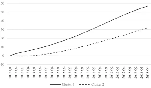
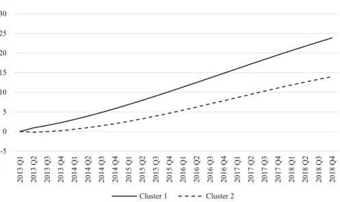
⁸

The trend of the quality- and spatial-adjusted price cluster means is shown in Fig. 4 and reveals the cumulated average price change of all dwellings allocated to the spe- cific price clusters, indexed to zero in 2013 Q1. While NUTS 3 regions allocated to price cluster 2 experienced slightly decreasing prices compared to the base quarter at the beginning and started to increase from 2014 Q1 onwards, for price cluster 1 a consistently positive price development is visible. However, over the entire obser- vation period both price clusters display a quite similar upward-sloping trend. Over the past 6 years, prices in price cluster 2 have been rising on average by 32% and in price cluster 1 even by 56.75%. As the price development in price cluster 1 is much steeper, these regions can be identified as highly demanded regions relative to regions allocated to price cluster 2.

Comparing regions assigned to price cluster 1 versus regions assigned to price cluster 2 by means of economic and socioeconomic data shows, that at the median

⁹

regions in price cluster 1 are larger with respect to the population as well as the working population. An even more pronounced trigger of the very strong price development in price cluster 1 might be the positive development of the population and working population over the whole observation period. Price cluster 1 regions experienced a 3.84% increase in population and working population rose by 2.5%. This definitely implies a higher demand for living space within the respective regions, resulting in higher prices. In contrast, price cluster 2 regions only had a very small increase in population of 0.97% and even suffered a loss of 0.91% in working population. This

8 A full list containing the classification of the 380 NUTS 3 regions is available upon request.

9 The median is used instead of the mean in order to prevent outliers from distorting the cluster values.

(19)

-10 0 10 20 30 40 50 60

2013 Q1 2013 Q2 2013 Q3 2013 Q4 2014 Q1 2014 Q2 2014 Q3 2014 Q4 2015 Q1 2015 Q2 2015 Q3 2015 Q4 2016 Q1 2016 Q2 2016 Q3 2016 Q4 2017 Q1 2017 Q2 2017 Q3 2017 Q4 2018 Q1 2018 Q2 2018 Q3 2018 Q4

Cluster 1 Cluster 2

Fig. 4Price index, investment market. The figure plots the mean cumulative percentage price change for dwellings allocated to the individual price clusters. The price changes are presented as the coefficients of the time dummy variable of a quality- and spatial-adjusted GAMLSS regression. To cluster the index values, the partitioning around medoids (PAM) algorithm was used. The data consists of 1,476,592 observations on the residential investment market. The sample period is 2013 Q1–2018 Q4

very small increase in demand might to some extent be responsible for the lower price

development in price cluster 2. However, as prices in price cluster 2 have also been

rising not negligibly, other price drivers than the pure demand for space must be an

issue. Regions allocated to price cluster 1 are furthermore characterized by a higher real

GDP, lower unemployment rates and a higher disposable household income compared

to price cluster 2. While in 2018 the median real GDP in price cluster 1 was about e5.2

million, regions in price cluster 2 only had a median real GDP of e4.3 million. It is

not surprising, that prices have had a larger growth in more productive regions as this

factor is a strong demand indicator and thus correlates with population changes. From

2013 to 2018 real GDP growth is observed for both price clusters, with the median real

GDP in price cluster 1 increasing by 10.3% and 8.42% in price cluster 2. The generally

flourishing economic conditions can also be observed by decreasing unemployment

rates and increasing disposable household income. While the unemployment rate of

2.67% in price cluster 1 is lower than in price cluster 2 with 3.28%, it is to note that the

decline in the unemployment rate is more pronounced in price cluster 2. The same is to

observe for the disposable household income. While the median disposable household

income of e48.43 thousand in price cluster 1 is higher than in price cluster 2 with

e43.29 thousand, the increase in price cluster 2 is stronger. The relatively stronger

development of the unemployment rate and the disposable household income in price

cluster 2 is not surprising, as these regions started with relatively weak levels for the

calculation of the growth rates. The relative strong decrease in the unemployment

rate in price cluster 2 and the relative strong increase in disposable household income

in combination with real GDP growth might somehow indicate that smaller regions,

in terms of population, with still very low disposable household income are in the

(20)

progress of slowly adjusting to the larger and economically stronger regions. This favourable economic development in rather small regions contributed to the upward sloping price development in price cluster 2 without strong gains in population and working population. There is no doubt that the prevalent situation on the investment market in general, with very low mortgage rates and sparse alternative investment opportunities played a significant role for the overall positive price development.

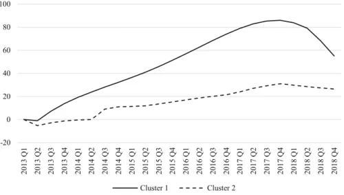
Assigning the regions to clusters by their liquidity development, which is based on the time it takes to sell a dwelling within the respective regions, displays a different pattern but also higher index values at the end of the observation period. As shown in Fig. 5, for regions assigned to liquidity cluster 2, liquidity was worse than in the base quarter in 14 out of 23 quarters. From 2014 Q1 onwards liquidity in liquidity cluster 2 was declining, i.e. marketing time in the respective regions was getting longer.

Liquidity hit the bottom in 2016 Q2, exceeded the level of the base quarter in 2017 Q4 and finished with a plus of 45.48% in 2018 Q4. Regions assigned to liquidity cluster 1 experienced a similar process. Though liquidity in liquidity cluster 1 never declined below the level of the base quarter, it was rather stagnating from 2014 Q1 until the end of 2016. The stagnating liquidity development might to some extent be caused by the sharp increase in building completions between 2013 and 2016. According to the Federal Statistical Office (2019a) building completion of dwellings has been rising from about 188 thousand in 2013 to about 236 thousand in 2016. As in this period the high demand for dwellings faces increased supply, liquidity remains rather constant.

Afterwards liquidity experienced a sharp increase, finishing with a plus of 75.05%

in 2018 Q4. Hence, over the entire observation period dwellings became on average more liquid in both liquidity clusters.

Taking a look at the economic and socioeconomic data of the considered regions, it is to observe, contrary to the price clustering, that liquidity was increasing most in regions with a lower median population as well as working population. The difference in population between liquidity cluster 1 and cluster 2 is way less pronounced than between the price clusters. The growth rates of these two variables, however, support the relative stronger liquidity growth in liquidity cluster 1. While the population in liquidity cluster 1 rose by 3.39% and the working population by 2.14%, liquidity cluster 2 experienced a rather small increase of 1.66% and 0.1%, respectively. As the plus in population generates more demand for space, the housing market gets tighter, hence the time it takes to sell a dwelling has been decreasing. In line with population, regions allocated to liquidity cluster 1 show a slightly smaller real GDP of e4.66 million compared to liquidity cluster 2 with e4.76 million. In comparison with price clustering, liquidity clustering results in way more similar clusters with respect to real GDP. The change in real GDP, that is more decisive when it comes to liquidity development, is higher in liquidity cluster 1 with 10.5% compared to liquidity cluster 2 with 8.79%. As with the price clustering these productivity gains coincide with the population development and hence result in higher demand for space leading to higher liquidity levels. For the unemployment rate, household disposable income as well as the respective growth rates the same picture as with price clustering is to observe.

The increase in liquidity was stronger in regions with a lower unemployment rate

and a higher disposable income. However, what might have triggered the liquidity

growth in liquidity cluster 2, though new demand for space in terms of population

(21)

-40 -20 0 20 40 60 80

2013 Q1 2013 Q2 2013 Q3 2013 Q4 2014 Q1 2014 Q2 2014 Q3 2014 Q4 2015 Q1 2015 Q2 2015 Q3 2015 Q4 2016 Q1 2016 Q2 2016 Q3 2016 Q4 2017 Q1 2017 Q2 2017 Q3 2017 Q4 2018 Q1 2018 Q2 2018 Q3 2018 Q4

Cluster 1 Cluster 2

Fig. 5Liquidity index, investment market. The figure plots the mean cumulative percentage change in liquidity for dwellings allocated to the individual liquidity clusters. The changes are presented as the coefficients of the time dummy variable of a quality- and spatial-adjusted Cox proportional hazards model.

To cluster the index values, the partitioning around medoids (PAM) algorithm was used. The data consists of 1,476,592 observations on the residential investment market. The sample period is 2013 Q1–2018 Q4

gains was relatively weak, was the pleasant development of the unemployment rate and disposable household income.

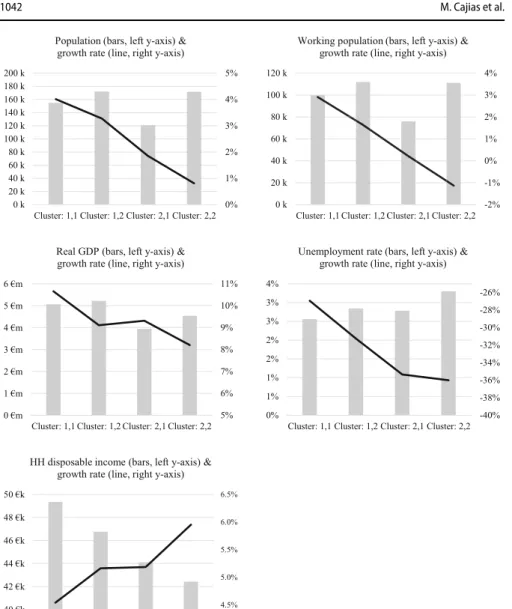
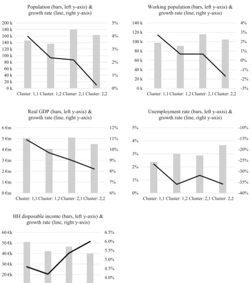
As mentioned above, a combination of the cluster ranks derived from the price and liquidity development is used in order to classify the 380 regions. For this purpose, the price cluster rank is regarded as the primary determinant and the liquidity cluster rank as the complementary secondary determinant, which enables a higher granularity in the classification and a more precise market assessment. Out of the 199 regions allocated to cluster 1 by price, 109 are as well allocated to liquidity cluster 1. Those regions can be declared as absolute “hot” markets, where an extraordinary price development is supported by a very strong liquidity development. The 128 regions assigned to cluster (2,2) are characterized as “cold”. Cluster (1,2) as well as cluster (2,1) can be found in the middle. Figure 6 summarizes the economic and socioeconomic data for the four possible cluster combinations on the investment market.

It is to observe that population and working population are the highest in regions with a relative weaker liquidity development irrespective of the price cluster, i.e.

clusters (1,2) and (2,2). These two clusters, however, also exhibit the highest unem-

ployment rates. Real GDP is highest in regions with a relative high price development

regardless of the liquidity cluster. Regions with a relative weaker price development

combined with a strong liquidity development, i.e. cluster (2,1), are characterized as

the smallest in terms of population, working population as well as real GDP. The

population and working population development clearly show the demand effect on

price and liquidity. The real GDP development shows a very similar picture. The

strongest population increase is to observe in regions that exhibit the strongest price

(22)

0%

1%

2%

3%

4%

5%

0 k 20 k 40 k 60 k 80 k 100 k 120 k 140 k 160 k 180 k 200 k

Cluster: 1,1 Cluster: 1,2 Cluster: 2,1 Cluster: 2,2 Population (bars, left y-axis) &

growth rate (line, right y-axis)

-2%

-1%

0%

1%

2%

3%

4%

0 k 20 k 40 k 60 k 80 k 100 k 120 k

Cluster: 1,1 Cluster: 1,2 Cluster: 2,1 Cluster: 2,2 Working population (bars, left y-axis) &

5%

6%

7%

8%

9%

10%

11%

0 €m 1 €m 2 €m 3 €m 4 €m 5 €m 6 €m

Cluster: 1,1 Cluster: 1,2 Cluster: 2,1 Cluster: 2,2 Real GDP (bars, left y-axis) &

-40%

-38%

-36%

-34%

-32%

-30%

-28%

-26%

0%

1%

2%

3%

4%

Cluster: 1,1 Cluster: 1,2 Cluster: 2,1 Cluster: 2,2 Unemployment rate (bars, left y-axis) &

4.0%

4.5%

5.0%

5.5%

6.0%

6.5%

38 €k 40 €k 42 €k 44 €k 46 €k 48 €k 50 €k

Cluster: 1,1 Cluster: 1,2 Cluster: 2,1 Cluster: 2,2 HH disposable income (bars, left y-axis) &

Fig. 6Socioeconomic data by cluster affiliation, investment market. The figure displays the socioeconomic data by cluster on the investment market. The NUTS 3 regions are allocated to a specific cluster by applying the partitioning around medoids (PAM) algorithm on the price and liquidity index values, respectively. The grey bars exhibit the actual values of the respective variables, labelled on the left y-axis. The black lines display the respective growth rates and are labelled on the right y-axis. The data consists of 1,476,592 observations on the residential investment market. The sample period is 2013 Q1–2018 Q4

and liquidity increases. Hence, more productive regions attract more people what in turn leads to more demand for space and consequently results in higher prices and higher liquidity. This is the case if the supply side cannot keep up. In contrast, the

“cold” markets experienced the weakest population growth. It is also to observe that

(23)

population as well as working population growth is more pronounced in cluster (1,2) than in cluster (2,1). This might indicate that population growth has a stronger impact on the price development than on the liquidity development. Furthermore, the “hot”

regions reveal the lowest unemployment rate as well as the highest disposable income.

Especially the household disposable income exhibits a strong variation between the clusters. While cluster (1,1) displays a median disposable household income of e49.34 thousand, cluster (2,2) achieves only e42.41 thousand. However, it seems as if the poor performing regions are trying to catch up. With a decline in the unemployment rate of 36% and an increase in disposable household income of 5.95%, cluster (2,2) regions are the best performers with regard to these two variables.

Regarding the spatial distribution of the clusters, as shown in Fig. 7, a strong concentration of regions allocated to cluster (1,1) and cluster (1,2) in the southern part of Germany emerges. While for Baden-Württemberg, Bavaria and south Hesse 90%, 70% and 85% of all regions are allocated to price cluster 1, the clustering approach displays a different distribution for the northern part of the country.

On the investment market, it seems like metropolitan areas with a prosperous eco- nomic outlook backed by strong fundamental data have large spillover effects on the surrounding regions, impacting their price and liquidity development. This effect can be observed for Berlin, Frankfurt, Hamburg, Hannover and Rostock. The increased demand for ownership in regions next to metropolitan areas might be caused by the increasing unaffordability of ownership within those metropolises and their outskirts.

Not surprisingly the share of eastern German regions is higher in price and liquidity cluster 2. The strongest concentration of eastern German regions allocated to price and liquidity cluster 2 can be found along the Czech and the Polish border. Of all eastern German regions represented in the sample, 61% are allocated to price cluster 2, while 67% are allocated to liquidity cluster 2. A similar pattern emerges for economically underdeveloped regions as defined by the Federal Ministry for Economic Affairs and Energy (2016), based on socioeconomic data like income and unemployment and the availability of infrastructure. Of those regions 68% are allocated to price cluster 2 and 67% to liquidity cluster 2. Since a proportion but not all of those regions are located in eastern Germany, a further geographical segmentation seems worthwhile. Interest- ingly, a majority of the economically underdeveloped regions which are assigned to price and liquidity cluster 1 is located in eastern Germany. This might be due to the fact that the price increase in more rural areas like those around Berlin and Rostock came only after the cities themselves became unaffordable and a large number of people began to demand dwellings which did not participate in a price rally beforehand. The western regions allocated to cluster (2,2) correspond very well to the regions defined as economically underdeveloped. Those are in particular the Ruhr Area which still suf- fers from the decline of its heavy industry, and the remote regions around the Emsland, in the far northwest of the country, and the regions close to the Danish border.