Determinants of Liquidity on the German Housing Market

(1)

Housing Market

Dissertation zur Erlangung des Grades eines Doktors der Wirtschaftswissenschaft

eingereicht an der Fakultät für Wirtschaftswissenschaften der Universität Regensburg

Vorgelegt von: Philipp Freudenreich MScRE, MScISIB Berichterstatter: Prof. Dr. Wolfgang Schäfers

Prof. Dr. Tobias Just

Tag der Disputation: 28. November 2018

(2)

II

List of Figures

Figure 2.1: Mean percentage change in price and time on market ... 17

Figure 2.2: Distribution of selected variables across purchasing power quantiles ... 19

Figure 2.3: Price index ... 25

Figure 2.4: Liquidity index investment market ... 26

Figure 2.5: Allocation of NUTS3 regions to price clusters, investment market ... 28

Figure 2.6: Allocation of NUTS3 regions to liquidity clusters, investment market ... 30

Figure 2.7: Rental index ... 32

Figure 2.8: Liquidity index rental market ... 33

Figure 2.9: Allocation of NUTS3 regions to price clusters, rental market ... 34

Figure 2.10: Allocation of NUTS3 regions to liquidity clusters, rental market ... 36

Figure 3.1: Mean survival function by market ... 60

Figure 3.2: Liquidity dispersion at city level ... 65

Figure 3.3: Non-linear effect of rent and age on coefficients ... 67

Figure 4.1: Average time on market in weeks in the seven largest German cities ... 75

Figure 4.2: Descriptive development of selected covariates along the TOM distribution ... 88

Figure 4.3: Estimated quantile regression coefficients of the quarterly dummies ... 95

Figure 4.4: Estimated quantile regression coefficient of the hedonic variables ... 100

Figure 4.5: Estimated quantile regression coefficients of the spatial gravity variables ... 105

Figure 4.6: Estimated quantile regression coefficients of the socioeconomic variables ... 107

(6)

List of Tables

Table 2.1: Variables and sources ... 16

Table 2.2: Overview of classification of the 161 NUTS3 regions ... 45

Table 3.1: Descriptive statistics ... 58

Table 3.2: Results Cox Proportional Hazards Model ... 63

Table 4.1: Variables and sources ... 84

Table 4.2: Descriptive statistics ... 86

Table 4.3: Average time on market in weeks per quantile ... 88

Table 4.4: Results of the Cox survival regression ... 91

Table 4.5: Results of the Censored Quantile Regression ... 115

(7)

1. Introduction

1.1 General Motivation

With a net asset value of € 4.81 trillions in 2015, the German residential real estate stock far exceeded the values of other European countries including France and the UK.¹ At that time, the market consisted of about 41.4 million dwellings.² Despite strong economic performance over the last decades, Germany developed into a nation of tenants. Voigtlaender (2009), Bentzien et al.

(2012), Lerbs and Oberst (2014), Kohl (2016), and Reisenbichler (2016), among others, describe reasons for this very distinctive market feature. Another peculiarity of the German market is the high proportion of private landlords. According to the GdW, roughly 37% of all dwellings are offered by about 3.9 million non-professional private landlords, while only 20% are offered by professional landlords.

Despite its tremendous size and widely dispersed ownership structure, the German residential market is relatively opaque and underresearched. This fact is mainly due to the lack of available data. Technological progress in terms of computational capacity, data gathering from internet sources, and the possibility to store large amounts of data have started to improve this situation.

Private data providers now offer micro data on a few million transactions on the residential investment and rental market. Although the quality of the data is not comparable to e.g. the US, as only asking prices and asking rents are observable, the new and large scaled data sets enable researchers to explore the market with a higher degree of detail. The data provider Empirica, for example, publishes quarterly price indices and price-bubble indicators. The digital market place Immobilienscout24 publishes the proprietary IMX index developed by Bauer et al. (2013) and even the Federal Statistical Office and the statistical offices of the federal states have started to publish monthly price and rent indices.

Irrespective of the individual provider, these indices share one particular finding. All of them reveal an increase in prices on the investment market, which far exceeds the increase on the rental market. Of course, the historically low interest rates fuel the demand on the investment market, while new landlords have stated to accept lower rental yields due to missing investment alternatives. Nevertheless, landlords are expected to hand over the price increase on the investment market as far as rental protection laws allow them to. German media publishes a record amount of articles about rising rents, the lack of affordable housing, and the threat of gentrification. However, the moderately rising rental price indices show no sign of surplus demand on the rental market.

The sole consideration of price to explain the movements on the residential market ignores the second integral component, when marketing a dwelling. The process of marketing a dwelling

1 Eurostat (2018)

(8)

starts with the introduction of the dwelling onto the market at a price (or monthly asking rent) determined by the seller (or landlord). With the introduction onto the market, the observation of the second integral component, which is the time it takes until a prospective buyer (or tenant) is willing to take the dwelling off the market and to pay the required price (or monthly amount of rent), starts. Contingent upon a matching of expectations, a market is able to function and the easier, thus faster this matching occurs, the shorter the timespan and consequently the higher the liquidity on the market. Typically, this matching will occur if the price (or asking rent) for the dwelling is supported by its particular location and building characteristics. Depending on the level of the demand in certain regions, buyers (or tenants) might start to tolerate higher prices (or rents). But as long as there is sufficient supply, the prospective buyer (or tenant) will continue to search the market and not rush into an undesired contractual agreement. In accordance with Fisher et al. (2003), the buyer (or tenants) is the provider of liquidity, as he has the financial resources to afford the dwelling and to convert it into cash (or a dividend yielding asset) for the owner. Only if it’s up to “take what you can get”, buyers (or tenants) will be accepting a price (or rent) which is exceeding their initial reservation price in no time.

Therefore, the aim of the dissertation is to emphasize the importance of a complementary detailed analysis of liquidity by underlining the significance of the component time on market, in order to get a more comprehensive understanding of the German residential real estate market. In this context, the dissertation examines liquidity solely with a time-based measure and does not include transaction cost, price, or volume measures.

Internationally, and in particular on the US residential real estate market, hedonic pricing is a very extensive field of research, going back to Kain and Quigley (1970) and Rosen (1974), among others. The combined analysis of price and time until sale goes back to Cubbin (1974), among others. Traditionally, the very transparent US market with its availability of high quality data gives room for inventions regarding modelling techniques. In the field of real estate hedonic pricing, a number of articles concludes that the inclusion of spatial variables improves the explanatory power of the model e.g. Goodman and Thibodeau (2007), Turnbull and Dombrow (2006), Pavlov (2000), Fik et al. (2003), and Bourassa et al. (2010), among others. Smith (2010) was the first to include district dummies and Cartesian coordinates as well as a distance variable in the context of liquidity analysis. The Quantile Regression (QR) approach, going back to Koenker and Bassett Jr. (1978), has been applied in the field of real estate pricing on the US market by Zietz et al. (2008), Farmer and Lipscomb (2010), Mak et al. (2010), and Liao and Wang (2012), among others. To use the model for the estimation of time on market, censoring in the data has to be taken into account. Due to insufficient computational capacity, this has not yet been possible. Thus, to the best of the author’s knowledge, the Censored Quantile Regression (CQR) has not yet been introduced to academic literature regarding real estate liquidity analysis.

(9)

On the German residential market, only the pricing aspect of residential real estate has received some form of attention in academic literature see Maennig and Dust (2008), Bischoff (2012), Kajuth et al. (2013), Belke and Keil (2018), among others. Ahlfeldt and Maennig (2010), Brandt and Maennig (2011), and Brandt et al. (2014), among others, introduced spatial variables and spatial gravity variables to the field of hedonic residential real estate pricing on the German market. However, they only concentrate their studies on one specific city. In the field of hedonic pricing, contemporary econometric models like the Quantile Regression and the Generalized Additive Models for Location Scale and Shape (GAMLSS) were introduced to the German market by Thomschke (2015) and Cajias (2018), respectively. However, in the field of liquidity analysis on the German residential real estate market, a substantial research gap exists.

The first paper of the dissertation enables the combined analysis of price and liquidity, by the introduction of quality- and spatial-adjusted hedonic liquidity indices to the German residential investment and rental market. The liquidity index for the rental market is able to reveal hidden demand, which is not represented by the price development. A subsequent clustering based on the index values identifies “hot” and “cold” regional markets. The clustering allows the deduction of investment strategies and assists public institutions when deriving policy measures regarding the residential market. Throughout the dissertation, liquidity is consistently defined as the inverse of time on market, as by Wood and Wood (1985). The estimation of time with econometric methods entails some particular features, like e.g. the absence of negative values or the existence of right censoring in the data. For the analysis of time on market this means, that some dwellings remain available on the market until the end of the observation period. Therefore, the second paper of the dissertation identifies and incorporates those features by exploring the determinants of liquidity by means of survival analysis, more precisely by the application of the Cox (1972) Proportional Hazards Model (PHM), which is able to estimate right censored data. While Kluger and Miller (1990) initially used the model for real estate liquidity analysis, the present paper adapts the PHM to the German market and, to the best of the author’s knowledge, it introduces spatial gravity variables to the field of residential real estate liquidity analysis on the German market. The application of a large scaled datasets allows the identification of heterogeneity across the cities and the deduction of liquidity patterns within the cities. The last paper of the dissertation builds upon the findings of the Cox PHM model in order to introduce the Censored Quantile Regression to the field of real estate liquidity analysis. To the best of the author’s knowledge, it is the first time, the model has been applied to the field in an international perspective. The advanced econometric model allows the examination of the determinants of liquidity on a very granular basis, as it explores the impact of different covariates for individual dwelling offerings across the time on market distribution. While the results confirm the proportional hazards assumption underlying the Cox PHM, they also reveal significant differences in the magnitude and the direction of the impact of individual characteristics on the time on market quantiles.

(10)

1.2 Research Questions

This section provides an overview of the three papers comprising the dissertation and the research questions addressed within those papers.

Paper 1: Closing the liquidity gap: Why the consideration of time on market is inevitable for understanding the residential real estate market

 How did prices on the residential investment and rental market develop according to official statistics?

 What is the current state of research on liquidity analysis for the residential real estate market?

 Is it possible to introduce a quality- and spatial-adjusted hedonic liquidity index to the German residential market?

 How did price and liquidity on the residential investment and rental market measured by quality- and spatial-adjusted hedonic indices evolve over the last five years?

 Did the indices for the residential investment and residential rental market develop differently?

 Is the strong demand pressure on the rental market captured by the rental price index?

 In how far do price and liquidity move together?

 Is the clustering of residential markets into “hot” and “cold” market states possible?

 How are the regions of each market cluster characterized? What similarities and differences do these regions share?

 Which investment strategies can be derived with respect to the individual market clusters?

Paper 2: Exploring the determinants of liquidity with big data – market heterogeneity in German markets

 What is the current state of research on liquidity analysis for the residential real estate market using the Cox Proportional Hazard Model?

 How did the liquidity analysis using econometric survival models evolve?

 Is it possible to adapt the Cox Proportional Hazard Model to the German residential rental market using a large scaled data set?

 Is it possible to adapt the Cox Proportional Hazard Model in order to include spatial information next to hedonic and socioeconomic variables and various fixed-effects?

 Does the inclusion of spatial gravity variables significantly increase the explanatory power of the model?

 What additional information can be derived by including the “atypicality” measure introduced by Haurin (1988) and the “degree of overpricing” introduced by Anglin et al. (2003)?

 What are the determinants of liquidity of rental dwellings in the largest seven German cities?

 Are there differences or commonalities across the seven largest German cities?

(11)

 Is it possible to derive geographic liquidity patterns for the seven cities?

Paper 3: Exploring the determinants of real estate liquidity from an alternative perspective – Censored Quantile Regression in real estate research

 How did advanced econometric survival analysis evolve in other fields of research?

 Is it possible to introduce the Censored Quantile Regression to the field of real estate liquidity analysis using hedonic, socioeconomic, and spatial variables and various fixed-effects?

 Is it possible to adapt the Censored Quantile Regression to the German residential real estate market using a large scaled dataset?

 What additional information does the model display for the determinants of liquidity of rental dwellings in the largest seven German cities by estimating each quantile separately?

 Does the direction and magnitude of the effect individual covariates have on liquidity change along the time on market distribution?

 Is it possible to confirm the proportional hazards assumption underlying the Cox PHM model?

 What information about the marketability of their current and future dwellings can landlords infer from the CQR results and how can they improve the marketability?

(12)

1.3 Course of Analysis

This section provides an overview of the course of analysis with regard to the research purpose, the study design, the authors, the submission details and conference presentations.

Paper 1: Closing the liquidity gap: Why the consideration of time on market is inevitable for understanding the residential real estate market

The aim of this paper is to emphasize the importance of time on market when analyzing the residential real estate market. Using 3,055,343 observations, the paper is the first, to the best of the authors’ knowledge, to introduce liquidity indices to the German residential investment and rental market. The paper is able to reveal the hidden demand on the rental market and creates clusters in order to summarize common market movements among the 161 observed regions and to facilitate the interpretation of the results. In addition, a higher tendency for spill over effects was found for the rental market.

Authors: Marcelo Cajias, Philipp Freudenreich, Anna Heller, and Wolfgang Schaefers

Submission to: Journal of Business Economics

Status: Under review

This paper was presented at the 2018 Annual Conference of the European Real Estate Society (ERES) in Reading, United Kingdom.

Paper 2: Exploring the determinants of liquidity with big data – market heterogeneity in German markets

This paper explores the determinants of liquidity on the residential rental market by examining 335,972 observations on the largest seven German real estate markets. The paper applies the Cox PHM in order to identify and measure those determinants. The model is adapted to include both absolute and relative spatial information in terms of coordinates and distance variables. To the best of the authors’ knowledge, this is the first paper to include spatial gravity variables to the field of real estate liquidity analysis on the German residential market in order to increase the explanatory power. The model is able to identify heterogeneity across the cities as well as liquidity patterns within the cities.

Authors: Marcelo Cajias and Philipp Freudenreich Submission to: Journal of Property Investment and Finance Status: Published in Volume 31, Issue 1

(13)

This paper was presented at the 2017 Annual Conference of the American Real Estate Society (ARES) in San Diego, USA and at the 2017 Annual Conference of the ERES in Delft, Netherlands.

Paper 3: Exploring the determinants of real estate liquidity from an alternative perspective – Censored Quantile Regression in real estate research

Based upon the findings of the previous paper, this study introduces an advanced econometric model to the field of real estate liquidity analysis in order to explore the determinants of liquidity with a higher level of granularity. To the best of the authors’ knowledge, this is the first paper to apply the Censored Quantile Regression in the field of real estate liquidity analysis. By using 482,196 observations on the seven largest German cities, CQR allows the identification and measurement of the impact an individual covariate has on time on market across the time on market distribution. The results reveal significant differences in the magnitude as well as the direction of the impact of individual characteristics on the time on market quantiles.

Authors: Marcelo Cajias, Philipp Freudenreich, and Anna Heller Submission to: Housing Studies

Status: Under Review

This paper was presented at the 2018 Annual Conference of the ERES in Reading, United Kingdom.

(14)

1.4 References

Ahlfeldt, G. and Maennig, W. (2010), “Substitutability and Complementarity of Urban Amenities: External Effects of Built Heritage in Berlin”, Real Estate Economics, Vol. 38 (2), pp.

285-323.

Anglin, P.M., Rutherford, R.C., and Springer, T.M. (2003), “The Trade-off Between Selling Price of Residential Properties and Time-on-the-Market: The Impact of Price Setting”, Journal of Real Estate Finance and Economics, Vol. 26 (1), pp. 95-111.

Bauer, T. K., Feuerschuette, S., Kiefer, M., an de Meulen, P., Micheli, M., Schmidt, T., and Wilke, L. H. (2013), “Ein hedonischer Immobilienpreisindex auf Basis von Internetdaten: 2007–2011“, AStA Wirtschafts-und Sozialstatistisches Archiv, Vol. 7 (1-2), pp. 5-30.

Belke, A. and Keil, J. (2018), “Fundamental determinants of real estate prices: A panel study of German regions”, International Advances in Economic Research, Vol. 24 (1), pp. 25-45

Benefield, J., Cain, C., and Johnson, K. (2014), “A review of literature utilizing simultaneous modeling techniques for property price and time-on-market”, Journal of Real Estate Literature, Vol. 22 (2), pp. 149-175.

Bentzien, V., Rottke, N., and Zietz, J. (2012), “Affordability and Germany’s low homeownership rate”, International Journal of Housing Markets and Analysis, Vol. 5 (3), pp. 289-312.

Bischoff, O. (2012), “Explaining regional variation in equilibrium real estate prices and income”, Journal of Housing Economics, Vol 21 (1), pp. 1-15.

Bourassa, S., Cantoni, E., and Hoesli, M. (2010), “Predicting House Prices with Spatial Dependence: A Comparison of Alternative Methods”, Journal of Real Estate Research, Vol. 32 (2), pp. 139-159.

Brandt, S. and Maennig, W. (2011), “Road noise exposure and residential property prices:

Evidence from Hamburg”, Transportation Research Part D: Transport and Environment, Vol.

16 (1), pp. 23-30

Brandt, S., Maennig, W., and Richter, F. (2014), “Do Houses of Worship Affect Housing Prices?

Evidence from Germany”, Growth and Change, Vol 45 (4), pp. 549-570.

Cajias, M. (2018), “Is there room for another hedonic model? The advantages of the GAMLSS approach in real estate research”, Journal of European Real Estate Research, Vol. 11 (2), pp. 204- 245.

Cox, D.R. (1972), “Regression models and life-tables”, Journal of the Royal Statistical Society:

Series B (Methodological), Vol. 34 (2), pp. 187-220.

Cubbin, J.S. (1974), “Price, Quality, and Selling Time in the Housing Market”, Applied Economics, Vol. 6 (3), pp. 171-187.

(15)

Eurostat (2018), “Balance sheets for non-financial assets (code: nama_10_nfa_bs)”, available at:

https://ec.europa.eu/eurostat/de/home (accessed: September 18, 2018).

Farmer, M. and Lipscomb, C. (2010), “Using quantile regression in hedonic analysis to reveal submarket competition”, Journal of Real Estate Research, Vol. 32 (4), pp. 435-460.

Fik, T.J., Ling, D.C., and Mulligan, G.F. (2003), “Modeling Spatial Variation in Housing Prices:

A Variable Interaction Approach”, Real Estate Economics, Vol. 31 (4), pp. 623-646.

Fisher, J., Gatzlaff, D., Geltner, D., and Haurin, D. (2003), “Controlling for the impact of variable liquidity in commercial real estate price indices”, Real Estate Economics, Vol. 31 (2), pp. 269- 303.

GdW Bundesverband deutscher Wohnungs- und Immobilienunternehmen e.V. (2014),

“Anbieterstruktur auf dem deutschen Wohnungsmarkt“, available at: https://web.gdw.de/uploads/

pdf/infografiken/2016/Anbieterstruktur.pdf (accessed: September 18, 2018).

Goodman, A.C. and Thibodeau, T.G. (2007), “The Spatial Proximity of Metropolitan Area Housing Submarkets”, Real Estate Economics, Vol. 35 (2), pp. 209-232.

Haurin, D.R. (1988), “The Duration of Marketing Time of Residential Housing”, Real Estate Economics, Vol. 16 (4), pp. 396-410.

International Real Estate Business School (IRE|BS), “Immobilienbestand und -struktur”, in: Just, T., Voigtlaender, M., Eisfeld, R., Henger, R., Hesse, M., and Toschka, A. (2017)

“Wirtschaftsfaktor Immobilien 2017”, Berlin, p. 19-48.

Kain, J.F. and Quigley J.M. (1970), “Measuring the value of housing quality”, Journal of the American Statistical Association, Vol. 65 (330), pp. 532-548.

Kajuth, F., Knetsch, T.A., and Pinkwart, N. (2013), “Assessing house prices in Germany:

evidence from an estimated stock-flow model using regional data”, Deutsche Bundesbank Working Paper, No. 46/2013, Deutsche Bundesbank, Frankfurt am Main.

Kluger, B.D. and Miller, N.G. (1990), “Measuring residential real estate liquidity”, Real Estate Economics, Vol. 18 (2), pp. 145-159.

Kohl, S. (2016), “Urban history matters: Explaining the German-American homeownership gap”, Housing Studies, Vol. 31 (6), pp. 694-713.

Koenker, R. and Bassett Jr., G. (1978), “Regression quantiles”, Econometrica, Vol. 46 (1), pp.

33-50.

Lerbs, O. and Oberst, A. (2014), “Explaining the spatial variation in homeownership rates:

Results for German regions”, Regional Studies, Vol. 48 (5), pp. 844-865.

Liao, W.C. and Wang, X. (2012), “Hedonic house prices and spatial quantile regression”, Journal of Housing Economics, Vol. 21 (1), pp. 16-27.

(16)

Maennig, W. and Dust, L. (2008), “Shrinking and growing metropolitan areas – asymmetric price reactions? The case of German single-family houses”, Regional Science and Urban Economics, Vol. 38 (1), pp. 63-69.

Mak, S., Choy, L., and Ho, W. (2010), “Quantile regression estimates of Hong Kong real estate prices”, Urban Studies, Vol. 47 (11), pp. 2461-2472.

Pavlov, A.D. (2000), “Space-Varying Regression Coefficients: A Semi-parametric Approach Applied to Real Estate Markets”, Real Estate Economics, Vol. 28 (2), pp. 249-283.

Reisenbichler, A. (2016), “A rocky path to homeownership: Why Germany eliminated large-scale subsidies for homeowners”, Cityscape: Ajournal of policy development and research, Vol. 18 (3), pp. 283-290.

Rosen, S. (1974), “Hedonic prices and implicit markets: product differentiation in pure competition”, Journal of Political Economy, Vol. 82 (1), pp. 34-55.

Smith, B.C. (2010), “Spatial Heterogeneity in Listing Duration: The Influence of Relative Location to Marketability”, Journal of Housing Research, Vol. 18 (2), pp. 151-171.

Thomschke, L. (2015), “Changes in the distribution of rental prices in Berlin”, Regional Science and Urban Economics, Vol. 51, pp. 88-100.

Turnbull, G.K. and Dombrow, J. (2006), “Spatial Competition and Shopping Externalities:

Evidence from the Housing Market”, Journal of Real Estate Finance and Economics, Vol. 32 (4), pp. 391-408.

Voigtlaender, M (2009), “Why is the German homeownership rate so low?”, Housing Studies, Vol. 24 (3), pp. 335-372.

Wood, J.H. and Wood N.L. (1985), “Financial Markets”, San Diego: Harcourt Brace Jovanovich.

Zietz, J., Zietz, E.N., and Sirmans, G.S. (2008), “Determinants of house prices: a quantile regression approach”, The Journal of Real Estate Finance and Economics, Vol. 37 (4), pp. 317- 333.

(17)

2. Closing the liquidity gap: Why the consideration of time on market is inevitable for understanding the residential real estate market

Abstract

This paper identifies the liquidity of dwellings, defined as the inverse of time on market, as an integral component when analyzing the residential market. Based on quality- and spatial-adjusted price and liquidity indices for about three million observations on the German residential investment and rental is clustered in order to summarize common market trends and to facilitate a regional interpretation. In that way, the study not only reveals the true demand on the rental market, but is able to identify “hot” and “cold” regions. This classification allows the deduction of investment strategies and enables a more precise drawing of policy implications. In addition, a stronger tendency for spill over effects was identified for the rental market.

Acknowledgement: The authors especially thank PATRIZIA Immobilien AG for contributing the dataset for this study. All statements of opinion are those of the authors and do not necessarily reflect the opinions of PATRIZIA Immobilien AG or its associated companies.

(18)

2.1. Introduction

On the residential market, the process of selling or renting out a dwelling comprises of two essential components. The first component is the introduction of the dwelling onto the market at a price (monthly asking rent) determined by the seller (landlord). The second component is the time it takes until a prospective tenant is willing to take the dwelling off the market and to pay the required price (monthly amount of rent). Contingent upon a matching of those expectations, a market is able to function and the easier thus faster this matching occurs, the higher the liquidity on the market. In the following, liquidity is defined as the inverse of the time on market (TOM) in accordance with Wood and Wood (1985). In this context, the study examines liquidity solely with a time-based measure and does not include transaction cost, price, or volume measures.

Typically, this matching will occur if the price (asking rent) for the dwelling is supported by its particular location and building characteristics. Depending on the level of the demand in certain regions, buyers (tenants) might start to tolerate higher prices (rent). But as long as there is sufficient supply, the prospective buyer (tenant) will continue to search the market and not rush into an undesired contractual agreement. In accordance with Fisher et al. (2003), the buyer (renter) is the provider of liquidity, as he has the financial resources to afford the dwelling and to convert it into cash (a dividend yielding asset) for the owner. Only if it’s up to “take what you can get”, buyers (tenants) will be accepting a price (rent) which is exceeding their initial reservation price in no time. Without a combined analysis of price (rent) and time, these exceptional levels of demand cannot be captured. Nevertheless, it is mainly price which is at the center of attention of market participants and captured by a variety of indices worldwide. To improve the assessment of the residential market, this paper provides quality- and spatial-adjusted liquidity indices for the residential investment and rental market, as complementary demand indices.

Over the last decade, the German residential real estate market has experienced significant changes. The fundamental economic data exhibits a growing GDP accompanied by historically high levels of labor demand. The consistently favorable macroeconomic situation and geopolitical events triggered high migration from within the European Union as well as from many conflict zones. In addition, the number of households has been increasing due to the social trend towards smaller households. Furthermore, interest rates for mortgages have been extremely low, resulting in higher affordability of home ownership. Unsurprisingly, this economic development led to booming demand for residential real estate. Despite rising building permissions and construction activity, building completions have been insufficient to meet the demand in many regions. The Federal Institute for Research on Building, Urban Affairs and Spatial Development (BBSR) has identified an increased demand of 272,000 new dwellings per year for the years 2015-2020.

According to the Federal Statistical office, dwelling completion was 216,727 in 2015, 235,658 in 2016, and 245,304 in 2017. The statistics show, that not in a single year since the BBSR published the study, enough new dwellings entered the market. As a consequence, vacancy rates fell below

(19)

sustainable levels in many regions and house prices as well as rents have experienced upside pressure. The official national house price index of the Federal Statistical Office reveals a national price increase of 19.7 percentage points (pp) for the last 5 years. According to the exclusive sample used for this study, which includes 973,164 observations on the investment market, asking prices increased by 33.1 pp on average within same period. Only 161 regions with more than 100 offers per quarter are included in the sample in order to avoid a bias stemming from those inactive markets. The Federal Statistical Office, however, includes all regions, irrespective of the activity of the market. A decomposition of the consumer price index published by the Federal Statistical Office reveals an increase in rents of a mere 5.7 pp for the last five years. Again, the current sample of 2,082,179 rental offers reveals a higher average increase of 13.5 pp within the same period. The price appreciation on the rental market seems innocuous in comparison to the one experienced on the investment market and even internationally, with the UK and the US undergoing a nationwide five-year rental increase of 10.8 and 16.0 pp, respectively. With a homeownership rate of 43% as of 2013, the first year covered by the current sample, more than half of the German population rent their homes. While Voigtlaender (2009), Bentzien et al.

(2012), Lerbs and Oberst (2014), and Reisenbichler (2016) discussed in detail the reasons for the extraordinarily low homeownership rate, research on the nationwide rental market is rather scarce, although not only the 2:1 ratio of available data for this study demonstrates the importance of the rental market. Simply based on the moderate appreciation in asking rents, it is hardly possible to make any inferences with regard to a tight rental market. Are the stories about property viewings with more than 50 competitors for the same flat only urban myths? Maybe the analysis of the liquidity on both residential markets reveals the somehow hidden demand. By only looking at the mean change in time on market, it seems as there is actually no difference between the investment and the rental market, as the liquidity improved by 52 and 46 pp respectively. An estimation of quality- and spatial-adjusted liquidity indices, however, exposes the real difference in market tightness.

As most other markets, the residential real estate market exhibits cyclical movements over time.

According to the seminal work of Kluger and Miller (1990) who developed a liquidity measure by using the Cox (1972) Proportional Hazards Model, housing prices and liquidity exhibit a positive correlation. Thus, prices and liquidity should match along “hot” and “cold” market states.

Krainer (1999) defines a market as “hot”' when prices are increasing, the time on market is short and transaction volume is above average. In contrast, decreasing prices, relatively long selling times and low transaction volumes point to a “cold” housing market. A positive correlation is found in Stein (1995), Berkovec and Goodman Jr. (1996), and Ortalo-Magné and Rady (2004) for instance. Follain and Velz (1995) and Hort (2000), among others, find a negative correlation.

While Stein (1995) and Genesove and Mayer (1997) reason the correlation with sellers' equity constraints, i.e. with frictions on the credit market, Krainer (1999) shows that “hot” and “cold”

real estate markets emerge due to search frictions and asymmetric information. Cauley and Pavlov

(20)

(2002) show evidence for the option value of homeowners and for nominal loss aversion.

Substantial deviations from these two market states might indicate speculative expectations by investors and landlords, adjustment processes or supply and demand changes. To detect these deviations is essential for real estate market participants, as it is otherwise impossible to build decisions correctly.

Literature in this field focuses predominantly on the US residential investment market, while academic research concerning real estate market movements on the German market is rather scarce. The lack of research on the German residential real estate market might be traced back to the fact, that micro data and computational power have not been sufficiently available only a few years ago. While most of this literature strand focuses on “hot” and “cold” market phases along the residential cycle, this paper aims to detect “hot” and “cold” market spots on a regional basis.

As one of the few papers on the German market, an de Meulen and Mitze (2014) identified “hot”

and “cold” spots on the Berlin residential market. In order to detect those, the authors exclusively investigated the price aspect of dwellings. In general, the movements on the residential real estate market are described primarily with price indices. On the German market, there are hedonic price indices provided by the Federal Statistical Office as well as indices provided by private companies like e.g. bulwiengesa and Immobilienscout24 (IMX). The methodology and data behind the IMX are described in Bauer et al. (2013). A complementary liquidity index, however, is missing.

Nevertheless, for central banks, policy makers, institutional investors, and private households it is essential to be aware of the liquidity momentum, as both indices might move in opposite directions, pointing to different market states. Thus, solely considering the price index for classifying a regional market might lead to incorrect investment strategies and policy implications. Therefore, this paper develops a quality- and spatial-adjusted price and a complementary liquidity indicator for the investment and rental market of 161 German regions.

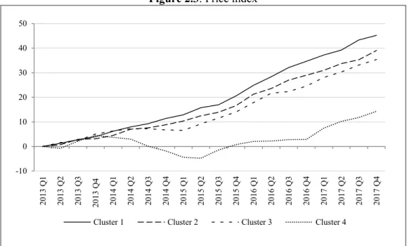
According to the indices, the regional housing markets are then clustered in order to reassess the assumption that prices and liquidity move together or whether their dynamic behavior exhibits frictions. For more than 25 years, bulwiengesa has been providing a clustering of German cities according to their size, measured by the number of inhabitants, the size of the office market and the importance of the city for the national as well as international real estate market.³ Heinrich and Just (2016) have noted, that those characteristics might not be entirely sufficient for analyzing the housing market and developed a solution which primarily includes information on the housing market and the population within those cities. While the approach of Heinrich and Just (2016) and the one presented in this paper both use a form of k-means clustering, the latter one does not directly cluster a variety of variables, but uses them for the preceding index calculation. In addition to the quality- and spatial-adjusted regional price and rent indices, the liquidity index is introduced as an additional layer, in order to cluster the regions. The indexing and two-

3 RIWIS database, Bulwiengesa AG

(21)

dimensional clustering on a regional level yields a very granular analysis of the German residential investment and rental market and allows the identification of “hot” and “cold” spots as starting points for the deduction of investment strategies. The findings should also be of interest to consumers of living space and policy makers trying to steer the residential market.

The study aims to answer the following questions regarding the residential market:

 How did prices on the residential investment and rental market develop according to official statistics?

 Is it possible to introduce a quality- and spatial-adjusted hedonic liquidity index to the German residential market?

 How did price and liquidity on the residential investment and rental market measured by quality- and spatial-adjusted hedonic indices evolve over the last five years?

 Did the indices for the residential investment and residential rental market develop differently?

 Is the strong demand pressure on the rental market captured by the rental price index?

 In how far do price and liquidity move together?

 Is the clustering of residential markets into “hot” and “cold” market states possible?

 How are the regions of each market cluster characterized? What similarities and differences do these regions share?

 Which investment strategies can be derived with respect to the individual market clusters?

The remainder of this paper proceeds as follows: The next section describes the dataset and the descriptive statistics. Section 2.3 presents a description of the econometric model, including the derivation of the hedonic price and liquidity indices as well as the clustering algorithm. Estimation results are presented and discussed in section 2.4. Section 2.5 concludes.

2.2. Data and descriptive Statistics

The sample used to estimate the price and liquidity indices combines three merged data sets. It contains information of 3,055,343 observations on the rental (2,082,179) and investment market (973,164) in 161 German regions from the first quarter of 2013 to the fourth quarter of 2017.

Information on the dwellings is gathered from various Multiple Listing Services (MLS) as collected from the Empirica Systems Database, containing real estate market data from the most important MLS providers. Hedonic characteristics of the dwellings contain the time on market as the number of weeks the dwelling was listed in the MLS calculated by the start and end date, the asking price in € for the investment market sample and the asking rent in € per month for the rental market sample due to a lack of transaction prices and contract rents. Nevertheless, a substantial bias is not to be expected, see e.g. Shimizu et al. (2012) and Lyons (2013), among

(22)

"with balcony", being 1 if the dwelling exhibits a balcony and 0 otherwise. Since the data is georeferenced, two spatial gravity indicators measuring the Euclidian distance of each dwelling to the geographical centroid of the ZIP and NUTS3 polygon in kilometers have been calculated.

NUTS3 regions correspond to the "Nomenclature of territorial units for statistics", which is a hierarchical system for dividing the economic territory in Europe. The NUTS3 regions cover small regions similar to counties or administrative districts. For the German case, those NUTS3 regions are either rather extensive counties containing many communities and smaller cities or urban districts. One example are the neighboring NUTS3 regions Munich city and Munich county.

The spatial gravity variables control for the spatial distribution of dwellings within a region.

Furthermore, the socioeconomic variables, purchasing power per household and the number of households at the ZIP code level, are extracted from the GfK-database. The population density per sqkm in a ZIP code area is then calculated in ArcGIS. The last source is Thomson Reuters Eikon, providing the 10-year interest rate for housing loans as a macro variable. The variables, their units and sources can be found in table 2.1.

Table 2.1: Variables and sources

Variable Unit Effect in the survival equations Source

Hedonic effects Spatial effects Socioeco nomic effects Empirica GfK ArcGIS Reuters

Asking price €    

Asking rent € per month    

Time on

market Weeks   



Living area M²    

Age Years    

Rooms Number    

With bathtub Binary    

With built-in

kitchen Binary   

 With car

space Binary   



With terrace Binary    

With balcony Binary    

With elevator Binary    

Newly built

dwelling Binary   

 Refurbished

dwelling Binary   

 Gaussian

longitude Coordinate 

 Gaussian

latitude Coordinate 



(23)

Distance to

ZIP centroid Km  

Distance to NUTS3 centroid

Km 

 Households in

ZIP HHs/ZIP 

 Purchasing

power of HHs in ZIP

€/HH/p.a./

ZIP 

 Population

density in ZIP

Persons/km²

/ZIP 

 IR for

housing loan 10 years

Effective interest rate in %





N 3,055,343

Notes: This table reports the unit, the type of effect, and the source of all variables included in the hedonic price and liquidity index calculations as well as the number of observations.

Figure 2.1 shows the mean asking price and time on market development on the investment and rental market from the first quarter of 2013 until the end of the observation period. It is visible that prices have been increasing accompanied by a diminishing time on market on both markets.

Hence, both indicators point to a boom phase on the German housing market, triggered by ongoing demand with supply lagging behind. Moreover, it is observable that transaction prices have been increasing considerably more than rents. While rents have been rising by a mere 13.5%, transaction prices have experienced a substantial growth of 33.1% over the last five years. Those figures indicate a particularly high demand on the investment market, probably triggered by constantly low mortgage rates on housing loans and a lack of interest bearing investment opportunities.

Figure 2.1: Mean percentage change in price and time on market

-10 0 10 20 30 40

2013 Q1 2013 Q2 2013 Q3 2013 Q4 2014 Q1 2014 Q2 2014 Q3 2014 Q4 2015 Q1 2015 Q2 2015 Q3 2015 Q4 2016 Q1 2016 Q2 2016 Q3 2016 Q4 2017 Q1 2017 Q2 2017 Q3 2017 Q4

Panel A: Percentage change in mean transaction price and rent

Δ asking price Δ asking rent

(24)

Notes: This figure plots the cumulative percentage change in mean transaction price and rent as well as the cumulative percentage change in time on market on the residential investment and rental market. The data consists of 973,164 observations on the residential investment market and 2,082,179 observations on the residential rental market. The sample period is 2013 Q1 to 2017 Q4.

However, it seems that the price development has not yet been fully absorbed by the rental market.

The relatively moderate growth in rents seems to only reflect the natural demand, which obviously was higher in cities. As landlords will try to pass on the rising prices on the investment market to their tenants, it might indicate further rental growth in the near future. Of course, rental protection laws prohibit landlords to hand over the entire increase in transaction prices to tenants in order to meet their target return. Asking exorbitant rent has been prohibited on the German market for years, not only since the introduction of the “Mietpreisbremse” in 2015. Because of lacking investment alternatives, new landlords somehow became acquainted to shrinking rental yields.

Nevertheless, time on market exhibits an enormous decrease of about 50% with an almost parallel development on both markets. Although price and rent have not experienced growth of equal magnitude, the similar development in time on market indicates considerably high demand on the rental market, which might also result in upward pressure on rents. To reason the similar drop in the time on market with relatively more supply on the rental market in relation to the investment market is rather less plausible, as newly built dwellings are usually offered on the investment market, before they appear on the rental market. Thus, this slightly controversial finding emphasizes the importance of focusing on both indicators – price and time on market – when analyzing the residential real estate market.

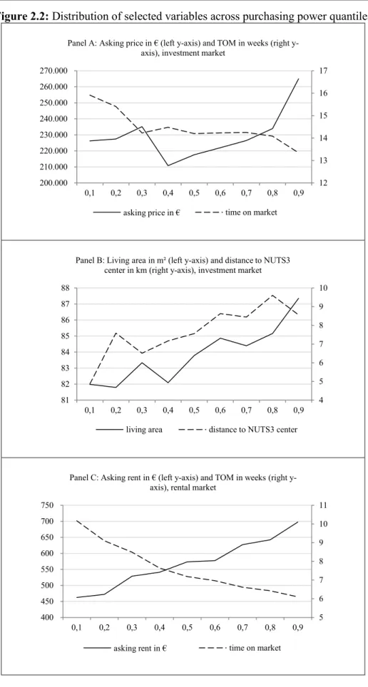
Figure 2.2 exhibits, that heterogeneity is omnipresent on the housing market. Panel A to D show, that households within different purchasing power quantiles demand a different price, living area, and distance to the city center. Furthermore, it is shown that the sales and letting process with respect to the marketing time varies.

-70 -50 -30 -10 10 30

2013 Q1 2013 Q2 2013 Q3 2013 Q4 2014 Q1 2014 Q2 2014 Q3 2014 Q4 2015 Q1 2015 Q2 2015 Q3 2015 Q4 2016 Q1 2016 Q2 2016 Q3 2016 Q4 2017 Q1 2017 Q2 2017 Q3 2017 Q4

Panel B: Percentage change in mean time on market investment and rental market

Δ investment TOM Δ rental TOM

(25)

Figure 2.2: Distribution of selected variables across purchasing power quantiles

12 13 14 15 16 17

200.000 210.000 220.000 230.000 240.000 250.000 260.000 270.000

0,1 0,2 0,3 0,4 0,5 0,6 0,7 0,8 0,9

Panel A: Asking price in € (left y-axis) and TOM in weeks (right y- axis), investment market

asking price in € time on market

4 5 6 7 8 9 10

81 82 83 84 85 86 87 88

0,1 0,2 0,3 0,4 0,5 0,6 0,7 0,8 0,9

Panel B: Living area in m² (left y-axis) and distance to NUTS3 center in km (right y-axis), investment market

living area distance to NUTS3 center

5 6 7 8 9 10 11

400 450 500 550 600 650 700 750

0,1 0,2 0,3 0,4 0,5 0,6 0,7 0,8 0,9

Panel C: Asking rent in € (left y-axis) and TOM in weeks (right y- axis), rental market

asking rent in € time on market

(26)

Notes: The figures plot the distribution of selected variables segmentd by nine purchasing power quantiles. The data consists of 973,164 observations on the residential investment market and 2,082,179 observations on the residential rental market. The sample period is 2013 Q1 to 2017 Q4.

Generally, relatively richer households can afford more expensive dwellings, prefer larger living areas, tend to live further away from the city center and spend less time on the search and matching process. These preferences are visible for the investment as well as the rental market. However, Panel C and D show, that the trend of the selected variables from the lowest to the highest purchasing power quantile is much smoother on the rental market. While the trend on the rental market is almost linear, it exhibits fluctuations on the investment market. Surprisingly, buyers living within zip codes with the lowest purchasing power (0.1-, 0.2-, 0.3-quantile) are asked to pay higher prices than the middle-income (0.4-, 0.5-, 0.6-quantile) groups. Another interesting fact is, that the range between the highest and lowest income group with respect to prices, living area and time on market is remarkably more pronounced on the rental market relative to the investment market. While on the investment market asking prices, living area and the time on market between the richest and poorest quantile vary by 17.1%, 6.5% and 16.2%, the differences on the rental market are much stronger with 50.9%, 23.6% and 40.0% respectively. This infers, that the participants on the rental market are much more diversified than those on the investment market.

2.3. Econometric Approach

The aim of a price index is to measure the price development over successive periods for the same quality-adjusted good. However, residential dwellings are not transacted periodically, but rather irregularly and even infrequently. Furthermore, residential real estate is extremely heterogeneous, both in terms of its physical characteristics and its location. Dwellings with different characteristics and in different locations might exhibit distinct price and liquidity dynamics in terms of volatility and cyclicality. Thus, idiosyncratic price and liquidity movements might be to

5 5 6 6 7 7 8 8 9 9

60 65 70 75 80 85

0,1 0,2 0,3 0,4 0,5 0,6 0,7 0,8 0,9

Panel D: Living area in m² (left y-axis) and distance to NUTS3 center in km (right y-axis), rental market

living area distance to NUTS3 center