On the Viability of Group Lending when Microfinance Meets the Market

(1)

On the Viability of Group Lending when Microfinance Meets the Market

A Reconsideration of the Besley––Coate Model

Lutz G. Arnold Johannes Reeder Susanne Steger

Abstract

Besley and Coate (1995) analyse the impact of joint liability and social sanctions on repayment rates when repayment enforcement is imperfect. Motivated by the microfinance industry’s move towards markets, we conduct an equilibrium analysis of the Besley–Coate model. We find that individual loan contracts may be used in market equilibrium, even though group lending entails the higher repayment rate and the lower break-even interest rate. This is because group lending causes potentially large deadweight losses. The market equilibrium is possibly characterised by financial fragility, redlining or rationing. Cooperation between borrowers and social sanctions imposed on each other in the case of strategic default turn group lending into the equilibrium mode of finance and ameliorate the market failures.

Journal of Emerging Market Finance 12(1) 59–106

SAGE Publications Los Angeles, London, New Delhi, Singapore, Washington DC DOI: 10.1177/0972652712473403 http://emf.sagepub.com

Lutz G. Arnold, Department of Economics, University of Regensburg, Regensburg, Germany. E-mail: Lutz.Arnold@wiwi.uni-regensburg.de

Johannes Reeder, Department of Economics, University of Regensburg, Regensburg, Germany.

Susanne Steger, Department of Economics, University of Regensburg,

(2)

JEL Classification: G21 Keywords

Microfinance, group lending, enforcement, social capital, social sanctions

Introduction

Two stylised facts of the microfinance industry are that (a) ‘microfinance meets the market’ (Cull et al. 2009) and that (b) group lending (GL) arrangements regularly incorporate enforcement mechanisms beyond joint liability including mechanisms that rely on social capital.

(a) Microfinance institutions (MFIs) increasingly rely on markets to fund loans. In Cull et al.’s (2009: 174) sample of 346 MFIs with combined assets of $25 billion (which is somewhat skewed toward for- profits) for-profit institutions (banks, credit unions and rural banks) account for 60 per cent of the assets, NGOs for 21 per cent and the non-bank financial institutions, which include both for-profits and non- profits, for 19 per cent. According to Reille and Forster (2008: 1), ‘[t]he entry of private investors is the most notable change in the microfinance investment marketplace’. There is a broad consensus that the huge demand for microcredit will continue to attract financial institutions with commercial interests: ‘[m]icrofinance will no doubt continue to expand and become part of the financial mainstream’ (Cull et al. 2009: 189).

This trend towards market funding poses a challenge to microfinance theory, calling for equilibrium models of the markets for microcredit and loanable funds.

(b) While early studies of GL emphasised the incentive effects of joint liability per se, it has become increasingly clear that other aspects of the lender–borrower relation are essential in making joint liability operative and in fostering high repayment rates (i.e., repayment proba- bilities) through other channels (see, e.g., Morduch 1999, Section 3, and Armendáriz de Aghion and Morduch 2000, Section 5). Some mechanisms are operative both with individual lending (IL) and with GL: con- tingent renewal provides incentives to invest in one’s reputation as a reliable borrower, and frequent repayments help substitute income for wealth as collateral. The mechanisms specific to GL ‘all rely on social

(3)

connections’ (Karlan 2007: F52). They include peer monitoring and cross reporting, which help overcome information asymmetries when borrowers are better informed about each other than lenders are.

Moreover, social connections between group members provide incentives to invest in one’s reputation as a reliable business partner in trade transactions and allow the exertion of direct social pressure to repay, in particular when otherwise group members become liable for one’s obligations.

The present article performs an equilibrium analysis of one of the seminal models in the theory of microfinance, viz., Besley and Coate’s (1995) (henceforth: ‘BC’) GL model. BC investigate the impact of joint liability and social sanctions in borrower groups on loan repayment rates. Project returns are sufficient to repay in their model, but due to enforcement problems, borrowers do not repay unless the penalty for default weighs heavier than the burden of repayment. Compared with IL, GL has two effects on repayment rates then. For one thing, it enhances repayment when one borrower is able and willing to stand in for a member of a group who does not repay. For another, however, liability for the repayment of the other members of her group potentially discourages a borrower from repaying at all when she would have repaid an individual loan. BC show that, in the absence of social sanctions, when pay-offs are independently and uniformly distributed and penalties for default are proportional to pay-offs, (depending on model parameters) either GL leads to a lower repayment rate than IL for all interest rates or the repayment rate is higher with GL than with IL only at low interest rates. By contrast, GL dominates IL in terms of repayment rates if there are sufficiently severe social sanctions. These results have been highly influen- tial in shaping the view that joint liability in groups succeeds in achieving high repayment rates only in conjunction with other enforcement mechanisms.

BC emphasise that their results ‘should not be taken as implying that group lending is better or worse than individual lending in any broader sense than repayment rates’ (p. 16), so ‘a more comprehensive analysis of the differences between the two lending schemes is an interesting subject for further research’ (p. 16). This is the aim of the present article: in line with stylised fact (a), we supplement the BC model with a minimum set of additional assumptions that enables us to characterise market equilibria. We determine the equilibrium lending type (IL or GL), which

(4)

maximises borrower utility, that is, minimises deadweight losses, subject to the break-even constraint for MFIs. In line with stylised fact (b), we take account of two kinds of social capital which help enforce repayments in groups, viz., cooperative behaviour in the repayment game (as in Ahlin and Townsend 2007, Subsection 1.3.2)¹ and social sanctions (as in BC, Section 4).

We show that there is even less scope for GL as the equilibrium mode of finance in the model with non-cooperative behaviour and without social sanctions than BC’s comparison of repayment rates suggests: for a broad range of model parameters, IL is used in equilibrium, even though GL achieves a higher repayment rate and breaks even at a lower interest rate. This is a straightforward consequence of the basic model mechanisms:

With IL, default occurs if, and only if, the return on investment is so low that it does not pay to repay a single loan. By contrast, with GL default potentially occurs when a borrower is willing to repay one loan but not two loans (viz., if, in addition, the other group member is not willing to repay a single loan). Hence, for a given interest rate, default occurs at higher project returns with GL and, given that penalties are proportional to project returns, causes larger penalties (i.e., deadweight losses) if it occurs. As a consequence, whenever the break-even interest rates with IL and GL are not too dissimilar, the equilibrium type of finance is IL.

Moreover, we show that the market equilibrium potentially displays the sorts of allocation failure familiar from the literature on asymmetric information in credit markets, viz., financial fragility, redlining or credit rationing. Cooperative behaviour and social sanctions not only enhance repayment rates (compared with the non-cooperative case without sanctions) but also turn GL into the equilibrium mode of finance and ameliorate the equilibrium allocation failures.²

The BC model is the ‘best known paper’ on enforcement in GL (Cassar et al. 2007: F86). It is one of the four models Ahlin and Townsend (2007) subject to their repayment rate-based test of models of joint liability lending (see also Armendáriz de Aghion and Morduch 2005:

297–298; Ghatak and Guinnane 1999: 209; Giné and Karlan 2008: 7;

Karlan 2007: F58). The popularity of the model in microfinance theory, jointly with stylised fact (a), provides a sound motivation for a reconsideration of the model with a focus on market equilibria. The most closely related papers are Rai and Sjöström (2004, 2010) and Bhole and Ogden (2010), which analyse repayment incentives in microcredit

(5)

markets with asymmetric information. A big advantage of these models is that, as they follow the mechanism design approach, any potential inefficiencies cannot be attributed to the use of non-optimal contracts.

Viewed from this perspective (see also Townsend 2003), an important caveat with regard to our results is that borrowers’ full liability for their peer group member’s repayment in conjunction with penalties which are proportional to pay-offs is evidently non-optimal in the BC model if one assumes that the penalties for default can be chosen freely: the threat of sufficiently severe penalties which will not be implemented in equilibrium ensures contractual repayment in all states of nature.

However, given that the BC model is concerned with imperfect enforcement of financial claims, the penalty function should be regarded as a measure of the (exogenous) limitations to enforcement. Moreover, in view of the fact that the underlying problem is to make credit available to the poor, the advice to use harsh punishments to ensure repayment seems to be of limited practical significance.

There is some empirical evidence that is supportive of the model and its basic mechanisms. First, the performance of different lending types in the BC model depends on how well they cope with the problem of limited enforcement of financial claims. That such enforcement problems are prevalent in countries where microfinance is used extensively is a well-documented fact. For instance, in Ahlin et al.’s (2011) sample of 373 MFIs from 74 countries, the mean time required to enforce a contract (taken from the World Bank’s Doing Business database) is 645 calendar days. Second, the model predicts that social capital enhances repayments by fostering cooperative behaviour and making borrowers sensitive to social sanctions. Several variables have been proposed to proxy for the strength of social ties (i.e., associational social capital), for instance, geographical proximity and cultural homogeneity.

Wydick (1999) and Karlan (2007), among others, confirm that the average distance between group members negatively affects repayment.

Karlan (2007) also finds a positive role for cultural similarity, using a self-constructed cultural score. These findings have been corroborated by experimental evidence. For instance, in an experiment conducted in South Africa and Armenia, Cassar et al. (2007) find a strong positive impact of cultural homogeneity between group members on repayment performance. In Cassar et al. (2007) and Cassar and Wydick (2010), another variable that emerges as an important determinant of repayment

(6)

rates from experiments with non-enforceable repayments is personal trust (measured by an index constructed from responses to questions from the General Social Survey, whether others in society are trust- worthy, fair and helpful). Cassar and Wydick (2010: 728) find that trust raises repayment rates and argue that this is because ‘[G]eneral trust is important to cooperative play’. This is in line with our result that cooperation between group members improves the performance of GL.³ Third, there is evidence of the exertion of non-pecuniary social sanctions (i.e., behavioural social capital). In Karlan’s (2007) study, dropping out of a group with rather than without default makes it 3–6 times as likely that current members report a worsening of friendship, trust and willing- ness to engage in future sales or purchase transactions. Carpenter and Williams (2010) conduct an experiment among micro borrowers in Paraguay. They find that individuals incur costs of monitoring and send- ing negative messages in the experiment and that observed repayment problems are less severe in groups whose members are more ‘nosy’ in the experiment. A further noteworthy fact is reported by Bratton (1986) in his descriptive analysis of repayments on group loans and individual loans in credit schemes in Zimbabwe in the early 1980s: The repayment rate was substantially higher with GL than with IL in good times, but worse after the disastrous drought of 1982–1983. This is consistent with the BC model, in which the disadvantage of GL stems from the fact that GL discourages a borrower from repaying anything when she would have repaid a single loan. Finally, Ahlin and Townsend’s (2007:

F42) comparative analysis of different models of GL using the Thai BAAC provides partially favourable results for the BC model: ‘the Besley and Coate model of social sanctions that prevent strategic default performs remarkably well, especially in the low-infrastructure northeast region’. The piece of evidence that is most detrimental to the BC model stems from Giné and Karlan’s (2008) study of the Green Bank in the Philippines, where the conversion of half of their GL centres in Leyte (randomly selected) to IL had no effect on repayment rates.⁴ An objec- tion to this result is that studies based on data from different locations (e.g., Ahlin and Townsend 2007; Cassar and Wydick 2010) show that effects on repayment are not uniform across locations and contexts, so that it remains to be seen whether the type of liability turns out to be inessential in other places as well.

(7)

The article is organised as follows. The second section describes the model. In the third section, we recapitulate BC’s main results. The fourth section characterises the model equilibrium. The fifth section introduces cooperative behaviour and social sanctions. The last section concludes.

Details of the algebra are delegated to Appendices 1 and 2.

Model

This section describes the model. We focus on the model with independently and uniformly distributed pay-offs, with proportional, non-pecuniary penalties for default, and, for now, with non-cooperative behaviour in the repayment game and without social sanctions. Since the BC model is well known, the exposition is kept brief. The additional assumptions made in our equilibrium analysis are highlighted as Assumptions 1–3.

Risk-neutral borrowers without internal funds and without collateral are endowed with one project each. The project requires an input of one unit of capital. The pay-offs θ are independently and uniformly distributed on the interval [ , ]θ θ , where

0.

2> >

θ θ (1)

The cumulative distribution function is denoted by F( ) ( (θ = θ θ− )/

(θ θ− ) forθ θ θ≤ ≤ ). MFIs offer loans. At the time a loan is made, the pay-off θ is uncertain. Once realised, the project return θ is observable by both borrowers and MFIs. An IL contract entails a repayment r. GL consists of a loan of size 2 to a group of two borrowers and repayment 2r. When the repayment decision is made, borrowers are endowed with sufficiently high income (exceeding 2r) so that they are able to repay.

However, the enforcement of repayment is imperfect, so borrowers choose between repaying (completely) or not (at all). The penalty for default is p(θ) = θ/β, where

β>max {1, }.θ ⁵ (2)

(8)

The penalty function p(θ) can be regarded as a measure of the limitations on the enforcement of repayments.

There is a tension between the implicit assumptions that borrowers have a second source of income besides project returns that enables them to repay but does not affect the severity of the penalty. A sensible interpretation, given that this is a theory of availability of credit to the poor, is that a borrower could mobilise enough money to repay by selling her belongings, but the MFI does not expect her to do this even in the case of strategic default and so does not condition the penalty on the value of her belongings. This also explains why the borrower’s belongings are not used as collateral in the first place.⁶ As explained in the Introduction, the assumptions that a borrower is fully liable for the group loan if her peer group member decides not to contribute to the repayment and that the penalty is an increasing function of the project pay-off are crucial to the results. A brief discussion of optimal penalty schemes is in ‘Equilibrium’

section and in Appendix 2.

BC assume that the penalty consists of ‘two components’, ‘a mone- tary loss due to seizure of income or assets’ and ‘a non-pecuniary cost resulting from being “hassled” by the bank, from loss of reputation, and so forth’ (p. 4). Their focus on repayment rates makes an assumption as to the relative magnitudes of the two components dispensable. In the working paper version of this article, we assume that each of the two components is a constant proportion of the penalty. Here, for simplicity, we make the following assumption (as in Rai and Sjöström 2004: 220):

Assumption 1: The penalty p(θ) is non-pecuniary; it is a deadweight loss.⁷

The two borrowers in a group (i = 1, 2, say) play a non-cooperative two-stage repayment game. At stage 1, the strategies are: contribute r to the joint repayment 2r or not. If both choose to contribute, the pay-offs are q_i – r, where q_i is i’s realisation of q (i = 1, 2). If both choose not to contribute, the pay-offs are q_i – p(q_i) (i = 1, 2). If borrower i chooses to contribute and j (≠ i) does not, i decides, at stage 2, whether she repays 2r alone or not. If she repays, she gets q_i – 2r and j gets q_j. If not, the pay-offs are q_i – p(q_i) (i = 1, 2).

To close the model from the supply side in the simplest possible fashion, we assume that the investors’ supply of funds to the MFIs is

(9)

perfectly elastic. That is, the MFIs’ cost of capital is exogenously given.

Assumption 2: The MFIs can raise any amount of capital at the con- stant cost of capital r (≥1).

An alternative interpretation is that we consider a lending scheme run by a non-profit development finance institution that can do with an average repayment r that falls short of the market return. It is straightforward to consider imperfectly elastic capital supply instead, and we will briefly come back to this issue in our discussion of credit rationing.

Due to perfect competition between MFIs, the equilibrium contract maximises expected borrower utility:

Assumption 3: The MFIs offer the (IL or GL) contract that maxim- ises borrowers’ expected utility subject to the constraint that they break even.

This is also a natural objective for an MFI funded by a development finance institution.

Repayment Rates

In this section, we briefly recapitulate BC’s comparison of repayment rates with IL and GL in the absence of social sanctions.

With IL, borrower i defaults if, and only if, p(q_i) = q_i/b < r, that is, q_i < br. So the repayment rate (the probability of repayment) is

( ) 1 ( )

I

r F r − r

Π = − =

− β θ β

θ θ (3)

for θ β/ ≤ ≤r θ β/ .

Turning to GL, for pay-offs below br, a borrower prefers the penalty over repayment. For q_i no less than br but below 2br, borrower i is willing to repay an individual loan but not a group loan. For q_i ≥ 2br, the borrower prefers to repay two loans over default. If ^r>θ^{/ 2 ,}

( )

β borrowers are unwilling to repay two loans even if the maximum pay-off materialises. It turns out that such interest rates cannot occur in

(10)

equilibrium (cf. ‘Equilibrium’ section), so in the main text we restrict attention to interest rates

θ ≤ ≤r 2θ

β β (4)

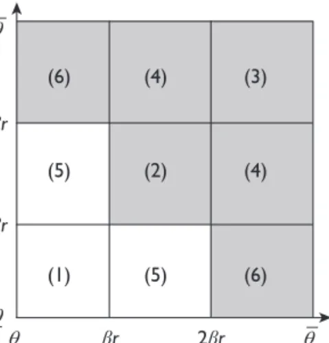
when considering GL. BC (p. 17) characterise the subgame-perfect Nash equilibria (SPNE) of the repayment game. Six cases have to be distinguished (see Figure 1):

(1) When both borrowers’ pay-offs fall short of br, then the group defaults.

(2) When both borrowers’ pay-offs are not less than br but insuffi- cient to induce them to repay two loans (i.e., less than 2br), both borrowers choosing to contribute is an equilibrium. Both borrowers deciding not to contribute is also an SPNE, which is however ruled out by BC (p. 7) on the grounds that it is Pareto-inferior. An alternative way to get rid of this ‘bad’ equilibrium is elimination of weakly dominated strategies (cf. Fudenberg and Tirole 2000, Subsection 1.1.2): The strategy not to contribute at stage 1 is weakly dominated by the strategy to contribute.

ȕT

ȕT ȕT

T ȕT T T

T T T

Figure 1. Cases that Lead to Repayment (shaded area) or Default (non- shaded area) as an SPNE with GL

Source: Developed by the authors.

(11)

(3) When each borrower is willing to repay two loans, one borrower repays 2r and the other free-rides.⁸

(4) When one borrower is willing to repay one loan but not two loans and the other borrower is willing to repay two loans, the former free-rides and the latter repays both loans.

In all these cases, the repayment per loan received by the MFI is the same as with IL.

(5) When one borrower is willing to repay one loan but not two (i.e., her pay-off is no less than br but less than 2br) and the other borrower’s pay-off falls short of br, then the group defaults.

This is the drawback of GL: joint liability discourages a borrower who would repay an individual loan from repaying anything at all.

(6) When one borrower’s pay-off is no less than 2br and the other borrower’s pay-off falls short of br, the high-return borrower stands in for her fellow group member. This is the advantage of GL.

The repayment rate is the cumulated probability of cases (2)–(4) and (6):

2

2 2 2

2

( ) 2[1 (2 )] ( ) [1 ( )]

3 4 2

( ) .

G r F r F r F r

r r

β β β

β βθ θ θθ

θ θ

Π = − + −

− + + −

= −

(5)

Comparing the repayment rates in (3) and (5) yields BC’s (p. 8) main result:

Proposition 1 (Besley and Coate 1995): (i) Suppose 1.

3 θ

β ≥ (6)

Then

( ) ( ) for

G r I r r 3θ

Π ≥ Π ≤ β ,

and vice versa. (ii) if θ β <^{/ 3}

( )

^1,Π_I(r) > Π_G(r) for all r ≥ 1.

(12)

Here and in what follows, we illustrate our results using a simple example⁹:

Example: Let θ =0.6,θ=5.5,β=1.2. Equation (4) becomes 0.5 ≤ r ≤ 2.2917. The condition of part (i) of Proposition 1 is satisfied:

( )

/ 3 1.5278 1.

θ β = ≥ The repayment rate is higher with GL or IL, depending on whether r < 1.5278 or r > 1.5278, respectively.

Equilibrium

This section characterises the model equilibrium. We show that the scope for GL is more restricted than a comparison of repayment rates suggests:

For a wide range of model parameters, IL is the equilibrium mode of finance, even though GL gives rise to a higher repayment rate at the break-even interest rate. We also demonstrate that the equilibrium possibly displays financial fragility, redlining (if there are multiple borrower classes) or credit rationing (if capital supply is imperfectly elastic).

Expected Repayments

From (3), the expected repayment per loan made with IL is

( ) ( )

²

I I

r r

R r r r β θ

θ θ

− +

≡ Π =

− (7)

for θ β/ ≤ ≤r θ β./ R_I(r) is hump-shaped with a maximum of RI^max≡ /(2 at /(2

RI(θ β)) r =θ β) .From (5), the expected repayment per loan made with GL is

2 3 2

2

3 4 2

( ) ( )

G G

r + r r

R r r r − β βθ θ θ θ

θ θ

+ ( − )

≡ ∏ =

( − ) (8)

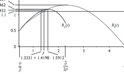
for θ β/ ≤ ≤ ( )r θ β ./ 2 R_G(r) is a hump-shaped function over the interval in (4) with a maximumRG^maxat an interest rate rG^max between θ β/ 3( )and θ β / 2( )(see Appendix 1). As in other models of imperfect enforcement,

(13)

for both lending types the impact of a further increase in the interest rate on expected repayment becomes negative as the interest rate grows large. Here the maximum expected return is unambiguously higher with IL than with GL:

Proposition 2: R_I^max> R_G^max.

Proof: From the definition of expected repayment, R_I(r) > R_G(r) if, and only if, Π_I(r) > Π_G(r). (i) From Proposition 1, R r_I( )>R r_G( )for r>θ β/(3 ) if (6) holds. Using the fact that θ β/(3 )<r_G^max <θ β/(2 ), it follows that

( ) ( )

max max max max

I I G G G G

R >R r >R r =R

(cf. Figure 2). (ii) For θ β/(3 ) < 1,the assertion follows directly from the fact that Π_I(r) > Π_G(r) for all r ≥ 1.

For future reference, denote the common value of R_I(r) and R_G(r) at / as :ˆ

r= (3 ) θ β R

2 2

ˆ 9

R θ

β θ θ

≡ .

( − ) (9)

Further, denote the lowest interest rate that breaks even with IL (i.e., the smallest solution to R_I(r) = r) as r_I (if it exists, i.e., if ρ≤R_I^max).

Analogously, r_G is the lowest break-even interest rate with GL: R_G(r_G) (if R_G^max).

ρ ρ

= ≤

Example: In the example introduced in the preceding section, R_I(r) attains its maximum R_I^max =1.2861 at ^r⁼^θ^{/ 2}

( )

^β ⁼^2.2917,and R_G(r) attains its maximum R_G^max =1.1462 at r = 1.5912. The expected repayment at the intersection of the two curves (i.e., at r = 1.5278) is ^R^{ˆ 1.1432}= (see Figure 2).

Expected Utility and Equilibrium

All borrowers demand loans at any interest rate. For IL, this is because the cost of a loan (i.e., either the interest repayment or the penalty) is less

(14)

than the pay-off in every state of nature: min{q_i/b, r} < q_i. The same holds true for GL: In none of the cases (1)–(6) discussed in the previous section does a borrower i repay an amount that exceeds q_i. In order to determine borrowers’ expected utility, we have to make an assumption about the probability of being the borrower who repays or the free rider in case (3). The natural assumption is that each borrower has an equal chance of being the free rider:

Assumption 4: The probability of being a borrower who repays in case (3) under GL is 50 per cent for each borrower.¹⁰

For r such that (4) holds, borrowers’ expected utility is

2 2 2 2

2 (1 )

( ) 2 ( )

I

r r

U r β βθ βθ β θ

β θ θ

− + + −

= − (10)

with IL and, given Assumption 4,

3 3 2 2 2 2

2 2 3

2

4 4 )

( )

( ) 2 ( )

G

r r r

U r

β β θ β θ θ θθ

βθ θ θθ θ β θ

β θ θ

− + (2 − 2 + +

− − ) − (1−

= −

(11)

with GL (see Appendix 1).

4₎T 4₊T

T U

ș ȕ

ȕș ȕș

Figure 2. Example: IL versus GL Source: Developed by the authors.

(15)

According to Assumption 3, MFIs maximise borrowers’ expected utility subject to their break-even constraint. So an equilibrium of the model consists of a lending type (IL or GL) and an interest rate such that

1. the expected return on lending is r and

2. there is no other lending type–interest rate pair that yields a higher expected return and at least as high a level of borrowers’ expected utility.

If we interpret MFIs as for-profits, this is the natural notion of equilibrium for a competitive market: There are no unexploited profit oppor- tunities for profit-seeking lenders. If, by contrast, we think of a market that is dominated by not-for-profits, then equilibrium entails that the lenders put the money under their management to its best use: they cannot economise on their lending without worsening their borrowers’

position.¹¹ For the sake of simplicity, we assume that GL is chosen when both types of lending yield the same level of expected borrower utility.

The following proposition states the obvious fact that if it is possible to break even with IL but not with GL, then there is an equilibrium with IL.

Proposition 3: If RI^max≥ >ρ RG^max, (IL, r_I) is an equilibrium.¹²

Proof: From the definition of r_I, (IL, r_I) satisfies condition 1 in the definition of an equilibrium. The condition of the proposition implies that it is not possible to make positive profit with a GL contract. To achieve R_I(r) > r, an MFI must set an interest rate r > r_I. However, from (10),

( ) 0

U rI′ < for all r<θ β./ This proves the validity of condition 2 in the definition of an equilibrium.

Propositions 2 and 3 jointly provide one reason for the use of IL as the equilibrium mode of finance. From Proposition 2, the maximum return on lending is higher with IL than with GL. Therefore, if the cost of capital is high enough, GL does not break even and IL is used in equilibrium (Proposition 3).

(16)

When is GL Used in Equilibrium?

In this subsection, we address the more interesting question of which type of lending survives competition if GL can also break even, so that it cannot be ruled out as the equilibrium lending type on a priori grounds.

From the definition of equilibrium, the choice of the equilibrium mode of finance then depends on expected borrower utilities. The following result provides a constructive approach to finding equilibria in that case:

all one has to do is compare expected borrower utility (or, equivalently, the deadweight losses induced by the different lending types) at the minimum break-even interest rates.

Proposition 4: If RG^max ≥ ,ρ (IL, r_I) or (GL, r_G) is an equilibrium, depending on whether U_I(r_I) > U_G(r_G) or U_G(r_G) ≥ U_I(r_I), respectively.

Proof: Since R_I^max> R_G^max, both lending types break even for sufficiently high interest. By virtue of the definitions of r_I and r_G, both (IL, r_I) and (GL, r_G) satisfy condition 1 in the definition of an equilibrium.

To check the validity of condition 2, consider first the case U_I(r_I) > U_G (r_G). The proposition asserts that (IL, r_I) is an equilibrium. By the same reasoning as in the proof of Proposition 3, it is not possible to make a profit with IL at an interest rate r ≠ r_I. As for GL, since r_G is the lowest break-even interest rate, R_G(r) > r requires r > r_G. But such interest rates do not attract customers:

U_G(r) < U_G(r_G) < U_I(r_I),

where use is made ofU rG′^{( ) 0}< for all r that satisfy (4) (see Appendix 1).

Thus, given IL at r_I, it is not possible to achieve a repayment above r and attract borrowers with either a different IL contract or GL. The case U_G (r_G) ≥ U_I(r_I) is treated analogously. MFIs have to charge an interest rate r > r_G in order to get a repayment R_G(r) > r with GL. SinceU rG′^{( ) 0}< , there is no demand for such contracts. Since R r_I′( ) 0 and> U r_I′( ) 0,< an IL contract that yields R_I(r) > r requires r > r_I and, therefore, does not attract customers either:

U_I(r) < U_I(r_I) ≤ U_G(r_G).

(17)

In Appendix 1, we show that the arguments go through without modification when r is not in the interval in (4).

We are now in a position to prove our first main result: GL may not be used in equilibrium, even though it breaks even at a lower interest rate and leads to the higher repayment rate at the break-even interest rate than IL. This will happen if the cost of capital r is less than, but sufficiently close to, Rˆ:

Proposition 5: Let condition (6) of Proposition 1 be satisfied and ^R^{ˆ 1.}>

Then there exists ρˆ<Rˆ such that for r in the interval ( ,ρˆ Rˆ], (IL, r_I) is an equilibrium, even though r_G ≤ r_I and Π_G(r_G) ≥ Π_I (r_I).

Proof: Define D_I (r) and D_G(r) as the expected penalties with IL and GL, respectively:

2 2 2

( ) 2 ( )

I

D r β r θ β θ θ

= −

− (12)

and

3 3 2 2 2 3

2

5 4 2

( ) 2 ( )

G

r r r

D r β β θ βθ θ

β θ θ

− − +

= − (13)

(see Appendix 1). From (12) and (13), the expected penalty is strictly higher with GL than with IL at r=θ β/(3 ) if, and only if, θ/3>θ (see Appendix 1). The validity of this inequality follows from (2) and (6). By continuity of the polynomials in (12) and (13), D_G(r) > D_I(r) for r less than, but sufficiently close to, θ β/(3 ). It follows that there exists ρ^ˆ<^R^ˆ such that D_G(r_G) > D_I(r_I) for r in the interval ( , ].ρˆ Rˆ Since the penalties are the only deadweight loss in the model, we have

E(q) – D_I(r) = U_I(r) + R_I(r) (14) and a similar equation for GL.¹³ From R_I (r_I) = R_G(r_G) = r and D_G(r_G) >

D_I(r_I), it follows that U_I(r_I) > U_G(r_G). From Proposition 4, IL is used in equilibrium, even though r_G ≤ r_I (since ρ≤^R^ˆ). From R_I(r_I) = R_G(r_G)

= r, R_G(r) ≡ Π_G(r)r, and R_I(r) ≡ Π_I(r)r, r_G ≤ r_I is equivalent to Π_G(r_G) ≥ Π_I(r_I).

(18)

Proposition 5 states that large deadweight losses potentially discour- age the use of GL in equilibrium even if it looks favourable in terms of repayment rates. This is a straightforward consequence of the basic model mechanisms, viz., the assumptions that a borrower is fully liable for the group loan if her peer group member decides not to contribute and that the penalty is an increasing function of the project pay-off. To see this, recall that the reason why GL is not unambiguously preferable to IL is that GL discourages the high-q borrower from repaying in case (5). The expected penalty on the high-q borrower, conditional on the occurrence of case (5), is

2 3

(2 ) ( ) 2 ,

E r r

F r F r r θ β θ β β

β β

 ≤ < 

 

  =

−

that is, one-and-a-half times the contractual interest payment.¹⁴ With IL, by contrast, the penalty q/b is always less than r, since the borrower repays whenever q/b ≥ r. Thus, the penalties under GL can be substantial if they are exerted.¹⁵

Example: From (10) and (11), U_G(r_G) ≥ U_I(r_I) for 1 ≤ r ≤ 1.0798, whereas U_I(r_I) > U_G(r_G) for 1.0798 < r ≤ 1.1432. That is, IL is used in equilibrium for ((1.1432 – 1.0798)/(1.1432 – 1) =) 44.27 per cent of the values of the cost of capital r for which GL breaks even at a lower interest rate than IL. For instance, let the cost of capital be r = 1.1. The minimum break-even interest rate is lower with GL than with IL: r_G = 1.3331

< 1.4198 = r_I(see Figure 2). The respective repayment rates are 82.52 per cent and 77.47 per cent. Nonetheless, the equilibrium entails IL, because this yields higher expected borrower utility: U_I(r_I) = 1.7338 > 1.7176 = U_G(r_G) (alternatively, the deadweight loss is lower: D_I(r_I) = 0.2162 < 0.2324 = D_G(r_G)). The expected penalty on the high-q borrower in case (5) with GL at zero profit is (3r_G/2 = ) 1.9996. This compares with penalties below r_I = 1.4198 with IL at zero profit.

To check whether the result that IL is used for a sizeable proportion of values of the cost of capital that imply r_G < r_I is robust, we investigate

(19)

a wide array of parameter values. We consider 11 different values for each of the parameters θ θ, and b:

θ ∈ {0.01, 0.2, 0.4, . . . , 1.8, 2}

θ ∈ {2.01, 2.7, 3.4, . . . , 8.3, 9}

b ∈ {1.01, 1.2, 1.4, . . . , 2.8, 3}

(with the cost of capital r yet to be specified). Of the resulting 1,331 parameter combinations, we pick those which satisfy (1), (2) and Rˆ 1≥ . For each of these 223 parameter combinations, we compute the critical level of the cost of capital ρˆ such that for r in the interval ( , ],ρˆ Rˆ IL is used in equilibrium even though GL has the lower break-even interest rate (i.e., r_G < r_I). We define

ˆ ˆ ˆ 1 P R

R

≡ −

− ρ

as the proportion of r-values which give rise to IL in equilibrium conditional on GL having the lower break-even interest rate for a given set of parametersθ θ^, and b. P ranges between 10.03 per cent and 100 per cent. The unweighted average over the 223 cases is 44.24 per cent.

This demonstrates that the use of IL in equilibrium despite the higher break-even interest rate is not an artefact of our running example. It happens for about half the r-values that give rise to rG ≤rI.

Market Failure and Optimal Contracts

The market equilibrium possibly displays the types of market failure discussed in the theory of asymmetric information in credit markets.

This is a direct consequence of the hump shape of the expected repayment functions (cf. Figure 2). First, there is financial fragility in that a small change in a model parameter can lead to a discontinuous change in the equilibrium values of the endogenous variables: When r rises aboveRI^maxthe market breaks down completely, since the lenders’ return

(20)

expectations can no longer be met. Second, when there are several markets of the type described in the ‘Model’ section with possibly different parameter values, only borrowers in markets with RI^max ≥ρ will receive credit, the borrowers in the other classes are ‘redlined’.

Third, if contrary to what has been assumed so far, the supply of capital is an imperfectly elastic function of r, then credit rationing occurs when the supply of capital at RI^max falls short of demand. Lenders then do not have an incentive to raise the interest rate despite the excess demand because that would decrease their expected repayment.¹⁶

Since the maximum expected repayment RI^max is achieved with IL here, financial fragility and credit rationing can only prevail when the equilibrium type of finance is IL, and individual loans are used before any borrower class is redlined as r rises. As will become clear in the sections ‘Social Capital’ and ‘Conclusion’, in the presence of cooperative behaviour or social sanctions these market failures can happen when GL is the equilibrium mode of finance.¹⁷

The definition of equilibrium entails that MFIs use the best (IL or GL) contract in terms of borrowers’ expected utility given the penalty func- tion p(q). Whether or not this is an optimal contract depends on whether or not the penalty function p(q) is considered exogenous or not. If it is not, that is, if p(q) can be chosen freely by the MFIs, then p(q) = q/b in conjunction with full liability for one’s peer group member’s loan is evidently not optimal: Given symmetric information, the first-best solution (no default, no penalties in equilibrium) can easily be achieved by means of the threat of sufficiently severe penalties which will not be implemented in equilibrium. For instance, r = r and p(q) = 2r will do.

Appendix 2 provides further discussion of the issue of optimal contracts (cf. Rai and Sjöström 2004; Bhole and Ogden 2010). However, it can be argued that assuming that p(q) can be chosen freely eliminates the sub- stance of the model. The model is about making loans in an environment with imperfect enforcement of financial claims. So the penalty function p(q) should be considered as a measure of the prevailing difficulties of enforcing contractual payments, and if p(q) can be chosen freely, the problem vanishes altogether. Moreover, in view of the fact that the underlying problem is to make credit available to the poor, the advice that enforcement can be improved by means of harsh punishments seems to be of limited practical significance.

(21)

Social Capital

The analysis so far lends support to the widely held view that the scope for GL is rather limited if the sole characteristic of GL is joint liability.

However, as emphasised by Armendáriz de Aghion and Morduch (2000), among others, there are other dimensions to GL contracts. In this section, we introduce additional enforcement mechanisms to the model that rely on the use of social capital. We show that this not only improves expected repayments with GL but does so in a way that promotes the use of GL rather than IL in equilibrium.

Cooperative Behaviour

In this subsection, following Ahlin and Townsend (2007, Subsection 1.3.2), we assume that borrowers play the repayment game cooperatively rather than non-cooperatively:

Assumption 5: The borrowers 1 and 2 in a group repay if, and only if, 2r

≤ p(q₁) + p(q₂). They share the pay-offs q₁ + q₂ such that both get the same expected utility.

Using p(q) = q/b, it follows that the members of a group repay whenever q₁ + q₂ ≥ 2br. Equal expected utilities could be achieved, for example, by sharing q₁ + q₂ – min{2r, (q₁ + q₂)/b} equally for all possible realisations (q₁, q₂).

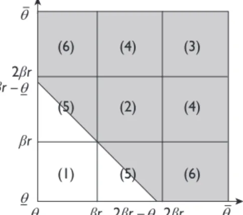
In terms of Figure 3, the two members of a group repay for (q₁, q₂) on and above the line with slope –1 through (br, br). As in the non- cooperative repayment game, the members of a group repay nothing in case (1) and 2r in cases (2)–(4) and (6). Cooperation is conducive to the repayment rate under GL because in the fields corresponding to case (5) in Figure 3, they default only in the area below the line q₁ + q₂ = 2br. One can infer from Figure 3 that the repayment rate with GL is higher than with IL: The repayments with GL or IL are the same in cases (1)–(4).

With GL, both group members repay in field (5) above the line q₁ + q₂ = 2br and in field (6), whereas both default in field (5) below the line q₁ + q₂ = 2br. With IL, by contrast, one of the two borrowers repays in cases (5) and (6). Since the area of the non-shaded portion of field (5) with GL

(22)

is less than half the total area of fields (5) and (6), given the uniform distribution of (q₁, q₂), the repayment rate is higher with GL than with IL (cf. Ahlin and Townsend 2007, Proposition 8, p. F24).

The repayment rate is 1 [(2− β θ θr− −) ] /[2(² θ θ− ) ]² , and the expected repayment is

2 2

2

( ) 2( )

( ) ( )

C

R r = − − r− r

−

θ θ β θ

θ θ (15)

for

θ ≤ ≤r θ θ2+

β β . (16)

For interest rates that satisfy (16), R_C(r) has the familiar hump shape (see Appendix 1). The interest rate that maximises the expected repayment is denoted as rC^max and the corresponding expected repayment as R_C^max (≡R r_C(_C^max)). In the main text, we restrict attention to interest rates which satisfy (16). In Appendix 1, we show that the analysis readily extends to interest rates r>(θ θ+ )/(2 )β . Notice that (16) implies (4): (θ θ+ )/(2 )β θ β< / . From (7) and (15), R_C(r) ≥ R_I(r) for all r such that (16) holds (see Appendix 1). Let r_C be the minimum

ȕT ȕT

ȕT

T T

TT ȕTŌT

ȕTŌT ȕT

T T

Figure 3. Repayment (shaded area) versus Default (non-shaded area) with Cooperative Behaviour

Source: Developed by the authors.

(23)

R_C(r) ≥ R_I(r) implies r_C ≤ r_I whenever break even with IL is possible (i.e., RI^max≥ρ). The deadweight loss per loan made with GL is

3 3 2 2 3

2

4 6 2

( ) 3 ( )

C

r r

D r = − +

−

β β θ θ

β θ θ (17)

for r such that (16) holds (see Appendix 1). The following proposition states that cooperation among the members of a borrower group is sufficient in order to turn GL into the equilibrium type of finance:

Proposition 6: (GL, r_C) is an equilibrium wheneverR_C^max≥ρ.

Proof: For r such that R_C^max ≥ >ρ R_I^max, GL is used in equilibrium because IL does not break even. So we can focus on the case R_I^max ≥ρ. The deadweight loss with GL D_C(r) satisfies

E(q) – D_C(r) = U_C(r) + R_C(r). (18) For r = r_C, this becomes E(q) – D_C(r_C) = U_C(r_C) + r. To achieve R_C(r) > r and U_C(r) ≥ U_C(r_C) with GL at r ≠ r_C, the deadweight loss must be smaller:

D_C(r) < D_C(r_C).

However, since r_C is the minimum break-even interest rate, R_C(r) > r requires r > r_C. Since D′_C(r) > 0 for all r>θ β/ (see Appendix 1), this implies

D_C(r) > D_C(r_C),

a contradiction. So there is no profitable GL contract that attracts borrowers.

Similarly, from (14) and (18), an IL contract with R_I(r) > r and U_I(r)

≥ U_C(r_C) must satisfy

D_I(r) < D_C(r_C)

and, as r_I is the minimum break-even interest rate, r > r_I. Without loss of generality, we can assume ^r≤θ^{/ 2 .}

( )

β This is because for any interest

(24)

rate above θ β/(2 ) that breaks even, there is a lower interest rate that yields the same expected repayment and, asD r > 0_I′( ) (from (12)), a lower deadweight loss. Consequently, (16) is satisfied so that (17) gives the deadweight loss with GL. It is straightforward to show that

( ) ( )

C I

D r < D r for all r≤θ β/(2 ) if θ/7.2749<θ (see Appendix 1).

Using r> ≥rI rC andD r_I′( ) 0> , it then follows that D_I(r) > D_I(r_I) ≥ D_I(r_C) ≥ D_C(r_C),

a contradiction. A different argument is needed to prove the assertion of the proposition when θ/7.2749<θ does not hold (one may skip this argument if one accepts this sufficient condition). Since this part of the proof is more complicated, it is delegated to Appendix 1.

The proof goes through without modification when we allow for ( )(2 )

r> θ θ β+ (see Appendix 1). So with cooperative behaviour, GL not only yields the higher repayment rate but also becomes the equilibrium lending type. This result lends support to the view that other mechanisms besides joint liability are needed to make GL the equilibrium mode of finance. Here it is the fact that borrowers cooperate (with one another, not with the lender) in planning their repayments which makes GL attractive for them.

The market equilibrium is potentially characterised by the market failures discussed in the preceding section. This follows immediately from the fact that the expected repayment function R_C(r) has the familiar hump shape, so that borrowers cease to get funds when r rises beyond

max

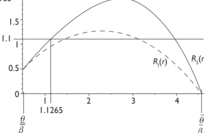
RC and positive excess demand at rC^max does not lead to an increase in the interest rate (when the supply of capital is imperfectly elastic). Thus, GL with cooperative repayment behaviour does not eliminate the market failures introduced in the preceding section. However, since R_C^max >R_I^max, the level of the cost of capital at which lending breaks down and the supply of capital in a rationing equilibrium are higher with GL (given positively and imperfectly elastic supply). In this sense, GL ameliorates the market failures.

Example: In the example with θ=^0.6,θ =^5.5, b = 1.2 and r = 1.1, the equilibrium interest rate is r_C = 1.1608. The repayment rate and expected utility rise to 94.76 per cent and 1.9007, respectively. R_C(r) achieves its maximum R^max =1.4603 at r^max =2.0087. While with

(25)

non-cooperative behaviour the market breaks down when r rises beyond 1.2861, an equilibrium exists for costs of capital up to 1.4603 here (see Figure 4). To illustrate the possibility of credit rationing in an equilibrium with GL, suppose there is a unit mass of borrowers and the supply of capital is S(r) = 0.6163r. Given zero profit for MFIs, the maximum feasible gross return is RS^max =^1.4603, and the corresponding supply of capital is S(1.4603) = 0.9. So in equilibrium 10 per cent of the borrowers are rationed, even though the expected project pay-off (θ θ+ )/2 3.05= exceeds the gross return needed to induce a capital supply equal to total demand significantly (S(1.6226) = 1). However, compared to the case of non-cooperative behaviour, the situation improves:

In the equilibrium without cooperation, IL generates the maximum gross return RI^max =^1.2861. The supply of capital is 0.7926, and 20.74 per cent of the borrowers are rationed.

Social Sanctions

Following BC (Section 4), we next introduce social sanctions to the model of the ‘Model’ section (returning to the assumption of

U

4_%T

4₊T

T

E E

E T

T TT

Figure 4. Example: IL versus GL with Cooperative Behaviour Source: Developed by the authors.

(26)

non-cooperative behaviour in the repayment game). BC’s main result in this regard is that if social sanctions are severe enough, GL yields a higher repayment rate than IL (BC, Proposition 3, p. 12). We show that, like cooperative behaviour among group members, social sanctions also make GL the equilibrium type of finance and ameliorate market failures.

We adopt the following simple specification of social sanctions:

Assumption 6: If one borrower i in a group decides to contribute at stage 1 of the repayment game and her fellow group member j decides not to contribute, then i imposes a sanction s > r on j. No sanctions are imposed otherwise.¹⁸

The presence of the sanction strengthens the incentives to contribute in the repayment game. For the cases defined in the section ‘Repayment Rates’ (cf. Figures 1 and 3), the following SPNE arise (r<θ β or r>θ β can be ruled out using the same arguments as in the section

‘Repayment Rates’):

1. Both borrowers choosing not to contribute is an SPNE. Due to the threat of penalties, both borrowers choosing to contribute is also an SPNE. As in the section ‘Repayment Rates’, the latter SPNE is ruled out on the grounds that it is Pareto-inferior.¹⁹

2. Both borrowers choosing to contribute is an equilibrium. The other SPNE, in which both borrowers decide not to contribute, is ruled out on the grounds that it is Pareto-inferior.

3. Contributing is a strictly dominant strategy at stage 1 for both borrowers. Neither tries to free-ride.

4. Contributing is a strictly dominant strategy for the borrower i with q_i ≥ 2br and a weakly dominant strategy for the other borrower.

The unique SPNE entails repayment.

5. This is the critical case for GL. Borrower 1, say, has a pay-off θ₁ in the interval (br, 2br), borrower 2’s pay-off falls short of br.

Contributing is a weakly dominant strategy for both borrowers at stage 1 (see Figure 5): if borrower 2 chooses not to contribute at stage 1 and borrower 1 decides to contribute, borrower 2 knows that borrower 1 will choose default at stage 2. Given Assumption 6, the social sanction s imposed on her weighs more heavily than the interest payment r (and the penalty q₁/b strengthens the case for

(27)

repayment). So repayment becomes an SPNE. Both borrowers choosing not to contribute is also an SPNE, which can be ruled out using elimination of weakly dominated strategies, however (the Pareto criterion is inconclusive here).

6. The unique SPNE entails that both borrowers contribute.

GL with social sanctions fares unambiguously better than GL with cooperative behaviour in terms of repayment rates. Repayment occurs except in case (1), so the non-shaded default area in Figure 3 shrinks.

This confirms Ahlin and Townsend’s (2007, Proposition 8, p. F24) finding that sufficiently severe social sanctions (‘unofficial penalties’) can enforce a higher repayment rate than cooperation. GL with social sanctions also dominates IL. Again, this follows from the fact that it reduces the default area to field (1) (whereas one of the two borrowers in a group defaults in the fields labeled (5) and (6) with IL, cf. Figure 1). We show in the following that this implies that lenders use GL, rather than IL, in equilibrium. The fact that GL with social sanctions dominates cooperation and IL is due to the fact that social sanctions are not carried out in equilibrium, so they do not cause any deadweight losses in addition to the penalties imposed by lenders.

The repayment rate becomes

2 2 2

2

2 2

( ) 1 ( )

( )

S

r r

r F rβ β βθ θ θθ

θ θ

− + + −

Π = − =