SFB 649 Discussion Paper 2016-034
Blooming Landscapes in the West?
German reunification - and the price of land.
Raphael Schoettler*
Nikolaus Wolf*
* Humboldt-Universität zu Berlin, Germany
This research was supported by the Deutsche
Forschungsgemeinschaft through the SFB 649 "Economic Risk".
http://sfb649.wiwi.hu-berlin.de ISSN 1860-5664
SFB 649, Humboldt-Universität zu Berlin
SFB
6 4 9
E C O N O M I C
R I S K
B E R L I N
Blooming Landscapes in the West? - German reunication and the price of land.
Raphael Schoettler1 and Nikolaus Wolf ∗2
1Department of Economics, Humboldt University Berlin
2Department of Economics, Humboldt University Berlin and CEPR
August 9, 2016
Abstract
German reunication was a positive market access shock for both East and West Ger- many. Regions that for 45 years had experienced a decline in population due to their loss in market access following the division of Germany after WWII were most strongly aected by this positive shock. We use an entirely new data set to analyse the eects of German reunication on the value of land in West Germany. We nd that regions in the immediate border area experienced a relative rise in land prices compared to regions outside a 100km radius from the border. At the same time we conrm the absence of a population eect (Redding and Sturm, 2008) even including rural boroughs. We nd that land values have adjusted more quickly than population and in some cases even overshot predicted long-run levels within the rst decade of reunication. We attribute this nding to the information and expectation component of land prices. Land values incorporate expectations about long- run equilibrium adjustments following reunication more swiftly, but rms and households are slower to react due to the costs of relocating. The results are consistent with empirical work on the positive eects of infrastructure projects on land values (Yiu and Wong, 2005;
Lai et al., 2007; Duncan, 2011).
Keywords: Economic Integration; Economic History; Regional Economics; Real Estate Markets.
JEL Classication Numbers: F15, N14, N94, R12, R30.
∗Address: Institut for Economic History, Unter den Linden 6, 10099 Berlin, Germany, telephone: +49 30 2093 5880, e-mail: r.schoettler@hu-berlin.de. The authors are grateful to Steve Redding for advice and suggestions, and to Oliver Salzmann, Maria Polugodina and Hefeng Fan for excellent research assistance, and seminar participants
1 Introduction
Germany reunied in 1990 following 45 years of dierent policy regimes. History oers a natural setting to empirically test the eects of this exogenous shock to market access for West Germany. Market access changed exogenously, but the policy regime remained stable in the West. This allows us to study market access as the driver of land value changes.
We nd that regions in the immediate border area experienced a relative rise in land prices compared to regions outside a 100km radius from the border. This nding is consistent with the theoretical predictions from the literature, although we do not nd the forecasted relative population growth in the border area. We attribute this to the information and expectation content of land values. In the spirit of an asset pricing model for land values prices adjust more rapidly to a change in relative location than population levels because prices contain expectations about future migration patterns.
The title of this paper refers to a speech delivered by chancellor Helmut Kohl on 1 July 1990 (Kohl, 1990) in which the term Blooming landscapes originally refers to the former German Democratic Republic. We however study the eects on the West German border boroughs which experienced their own gradual decline since division.
What are the reasons behind the dierences in population density and land prices across regions? Do shocks play out similarly everywhere? Do (temporary) shocks to market access and policy regimes lead to new spatial equilibria? How are the gains from reunication distributed?
Is the eect of reunication the mirror image of division? Do land values and population levels co-move? Do land values evolve similarly across Germany? What are the drivers of house price growth? And are any eects persistent in the long run? These questions will guide the following analysis.
This paper attempts to shed light on the importance of history and path dependence for the location of economic activity. It relates to the theoretical literature on new economic geography and the existence of multiple equilibria and oers a new piece of evidence for the empirical relevance of this theory. We exploit variation in the intensity of the market access shock to analyse the dierent outcomes in land price changes. The size of the market access shock was such that the smallest boroughs experienced a market access increase equivalent to a 15-fold population increase.
General equilibrium economic geography models centre around the question how economic
activity is distributed spatially. Two eects work in opposite directions. Positive eects from ag- glomeration that manifest themselves in knowledge spillovers for rms, deeper consumer markets and shorter transport ways are balanced out by negative eects from congestion.
Immobile farmers and mobile industry workers result in Krugman's (1991) endogenous dif- ferentiation into core and periphery. Helpman (1998) substitutes farmers with the factor land, a view now widely shared and employed in this dissertation. The xed supply of land is the limiting factor in preventing all economic activity from concentrating in a single location. In addition, pollution, noise or rising crime rates are forces preventing all economic activity from concentrating in one area. As a region becomes more densely populated demand for housing rises and consequently the fraction of income disposable for consumption falls. Due to the challenge of measuring the two forces economic geography models often do not disentangle the agglomer- ation and congestion eect and focus instead on population changes as a net measure of the two opposing forces.
Likewise trade theory suggests that market access is a crucial driver of economic development.
Industries featuring increasing returns to scale or a greater reliance on supply chains tend to locate in regions with better markets access. The reunication of Germany constitutes a natural experiment to analyse the eects of an exogenous change to market access. The new data set allow us to consider the strength of these opposing forces. We exploit this relationship in considering the value of land which is the underlying fundamental of house prices.
Thereby, we are able to demonstrate that reunication led to a rise both in the level of land values and in the growth rates. The disaggregate data show that the gains from reunication are not evenly distributed. Regions closer to the former GDR experienced a relatively larger rise in land prices. Furthermore, rural areas in the border area did relatively better than cities.
This is because the reunication shock was in relative terms larger for them as their own market potential is smaller.
Reunication allows us to identify the market access shock without the concern of endogene- ity issues usually associated with empirical studies that consider more gradual trade liberali- sations. Several approaches have been employed to overcome this issue by exploiting variation in market access such as Amiti and Javorcik (2008) who consider rm location choice in China or Treer (2004) assessing the shock of the NAFTA free trade agreement between Canada and the U.S. These liberalisations tend to be incremental such as in the case of the NAFTA agree- ment between Canada and the U.S. that was preceded by a perioded of some trade activity and
lengthy negotation rounds.
In line with Donaldson and Hornbeck (2016) we rewrite the Redding and Sturm (2008) version of the Helpman (1998) model. This enables us to consider land values as the dependent variable.
Using a unique new data set on disaggregate land values we present an empirical analysis of the reunication eects. We do nd evidence that distance to border plays an important role in understanding the dynamics after reunication. A newly assembled data set on land values (Bodenrichtwerte) in the four federal states along the inner German border (Schleswig-Holstein, Lower Saxony, Hesse and Bavaria) is used to assess the impact of reunication on land values.
This paper exploits the exogenous variation in market access in a dierence-in-dierences setup. Reunication did have a positive eect on the value of land. This eect did however dier greatly between the considered subgroups. The separate consideration of distance to border and the classication into rural and urban boroughs matters. Arguing that population levels are slower to adjust while land prices react more quickly to expectations, We oer an explanation for the fact that Redding and Sturm document a large negative division eect, but did not nd a corresponding reunication eect. The theoretical predictions from the Helpman model are conrmed more convincingly with regard to land values. The cost of relocation of rms and households pose a hurdle to a speedy response of population levels.
The theoretical connection between market access and land values is clear. The empirical work has focused in particular on the link of land values and transport connections. Studies have documented positive changes in land values corresponding to announced infrastructure projects.
For the US and Hong Kong these price changes are incorporated into land values well before the completion of the infrastructure improvements (Yiu and Wong, 2005; Lai et al., 2007; Duncan, 2011).
But let us rst briey turn to the historical context. Disagreement amongst the allied nations about the setup of post-war Germany ultimately led to the division of Germany into East and West. The three Western allies France, the United Kingdom and the United States of America promoted an integration of West Germany into the Western hemisphere, but the Sowjet Union kept a rm grip over the Eastern territories that would later become the German Democratic Republic. The economic and political collapse triggered the break-up of the Sowjet Union 45 years later and brought about the peaceful reunication of Germany. When the GDR elites celebrated the 40th anniversary on 7 Oktober 1989 little did they expect the events that were about to unfold. Only a month later, following mass protests around the GDR, a press conference
unintenionally made the border permeable. Within a further eleven months the two Germanies were reunied. Reunication was arguably unexpected and occurred rapidly, thereby satisfying the conditions for an exogenous shock.
In reaction to the division of Germany and in particular following the construction of the wall West Germany decided to nancially support the periphery. The government aid to bor- der regions was at rst an unwritten practice, but the ocial government aid border regions act (Zonenrandgebietsfoerderungsgesetz) was put into eect in 1971 by the German parliament (Bundestag, 1971). Military considerations did play a role when the decision to keep the bor- der periphery populated was taken. The subsidies comprised a wide range of measures such as preferential treatment of companies located in the designated regions in the awarding of public contracts, tax breaks for rms as well as favourable depreciation options. In addition, social housing schemes were put in place and spending on infrastructure projects increased. This subsidy started to phase out following reunication due to the necessity to rebuild the East of Germany. Most subsidies had ceased to be granted by 1994. In this context the data allows me to consider the persistence of these subsidies.
The paper is organised as follows. After a brief presentation of the Helpman model we sim- ulate the eect of reunication on population levels and land values. We derive two predictions that we then take to the data. In line with Redding and Sturm we do not nd evidence for a systematically dierent population growth between the border region and the non-border region even including all rural boroughs below 20,000 inhabitants. As the Helpman model does only make long-run predictions about the equilibrium population distribution we have collected dis- aggregated land price data to assess the short-run eects of the fall of the Iron Curtain and the associated change in market access. We rearrange the Helpman model equations to derive an equation with the price of the non-traded amenity as the dependent variable. In the following section 3 we present the data set of standard land values. Section 4 focuses on the empirical test of the empirical predictions. A series of robustness checks follows in section 5 before section 6 concludes.
2 Theoretical framework
In the economic geography Helpman model of general equilibrium positive eects from ag- glomeration and congestion eects determine the distribution of economic activity across space.
Negative dispersion forces enter in the form of a xed supply of the non-traded amenity, which we choose to interpret as the xed supply of land. The equilibrium population distribution is de- termined endogenously through perfectly mobile labour thereby equalising the real wage across all regions. We calibrate the model parameters to the pre-reunication population distribution in West Germany and East Germany separately deriving one common real wage each in the West and in the East. Simulating the opening of the border We treat the two German states as one and compute the new long-run distribution of population.
The key equation relates population levels in region i to two measures of market access, housing supply and the real wage
Li =χ (F M Ai)
µ
σ(1−µ) (CM Ai)
µ
(1−µ)(σ−1) Hi (1)
where χ =ω−1/(1−µ)ξµ/(1−µ)1−µµ is a function of the real wage and a number of constants, F M A is a measure of rm market access and CM A is a measure of consumer market access.
We then proceed to calibrate the model using given parameter values from the literature for σ, µ and θ such that the observed 1988 population distribution is a solution of the long-run equilibrium price vector. Appendix 6 contains an overview of the parameter choices and the other model equations.
Let us rst consider the central equation derived from the Helpman model. Densely popu- lated areas exhibit higher price levels of the non-traded amenity Hi because the supply of land available is limited and can be treated as xed. Even in the more rural areas the administrative procedure needed to declare a piece of land as land ready for construction (Bauland) is complex and requires time. At least in the short and medium run the supply of land can therefore be treated as inelastic. Now an exogenous market access shock hits the system of equations and al- ters the relative attractiveness of boroughs. This induces future migration ows thereby bidding up the prices in some regions.
The simulation and calibration diers from Redding and Sturm in that all boroughs are considered here as opposed to focusing on cities alone. The Helpman model predicts that smaller boroughs are disproportionately aected by the same absolute market access shock.
In addition, the data suggest that the dierence between rural (population <5,000) and cities is much larger than the within city variation Redding and Sturm consider. We use the 1988 population distribution and calibrate the other model parameters. We then simulate the new
population distribution following reunication by solving the system of equations simultaneoulsy using MATLAB.
2.1 Simulation of reunication
Figure 1 depicts two maps of Germany. Figure 1a shows the calibrated price levels of the non- traded amenity in West and East Germany prior to reunication. We interpret the population distribution of 1988 as the given long-run equilibrium and calibrate the model parameters such that the real wage is equalised across all boroughs. West and East are treated as two separate countries with no population movement between them. Dark blue indicates the smallest land price level while dark red signies the highest values.
The agglomeration eects are particularly visible in the Rhein-Ruhr area, in the Rhein-Main region around Frankfurt and in the greater Stuttgart area. The wage equalisation yields a lower real wage for East Germany. The border is visible almost through the entire border stretch as it runs between the darker blue shaded areas in the East and the lighter areas in the West.
This is in part explained by the dierent overall population sizes. The higher overall population in the West leads to a higher real wage ceteris paribus. This in turn raises the price level for the non-traded amenity. The border between East and West visible in the price level should therefore not be overstated.
The major cities exhibit the highest price levels of the non-traded amenity. The maps derived from the model predictions conrm the observed population data: land prices are highest in the biggest cities. Agglomerations such as the Ruhr area and the greater Frankfurt region emerge.
Now simulating the opening of the border people move around and across the border to generate a new spatial population distribution equilibrium. The common real wage is now the same across East and West Germany. Comparing gures 1a and 1b we observe an apparent gravitation towards the centre of Germany. Preserving the stylised city-rural dierences the East-West gap disappears.
2.2 Theoretical predictions
The simulation of the market access shock from reunication on the model parameters allows us to formulate two theoretical predictions
1. Regions closer to the German-German border experience a positive population growth.
The eects declines monotonically as one moves away from the border.
(a)Calibrationpre-reunication(b)Simulationpost-reunication Figure1:SimulationHelpmanmodel:landvalueequilibrium
0102030
Mean Simulated Land Price Change (%)
<25 25-50 50-75 75-100 >100
By distance in km from the East-West Border Simulated Change in West German Land Prices
(a)
051015
Mean Simulated Population Change (%)
Rural Area City
Full sample split into Cities and Rural Areas Differences in Simulated Land Price Changes
(b)
Figure 2: Simulation Helpman model: reunication
2. A positive shock to a location's market access aects locations with a smaller population relatively more as the shock is larger relative to their own market potential.
These two predictions are summarised in gures 2a and 2b. The predicted overall long-run land value growth is close to 25% in the immediate border vicinity (025km). The eect then monotonically decreases with the mean land value growth in the group further than 100km away from the border being negative. We exploit this reversal in the empirical section and declare all boroughs within 100km of the border to be part of the treatment group whereas the boroughs outside 100km from the inner German border form the control group. The split between rural areas and cities conrms the second prediction. The market access shock of the border opening has a relatively larger eect on boroughs with a smaller initial population. The actual values in the simulation appear like prices, but cannot be easily interpreted in their magnitude. Depending on the choice of other parameter values one can arbitrarily obtain other values. Only the relative percentage changes matter.
As transport costs in the model are approximated by distances between boroughs, the area in the centre of the unied Germany becomes more attractive. We assume that travel links do exist, are available for use from day one of reunication, and travel times are identical across regions for the same distance.
We then proceed to test the predictions in section 4 using the new data on land values. But rst, we revisit the empirical exercise from Redding and Sturm to understand why they do not nd empirical support for a positive reunication eect.
2.3 Reunication and relocation
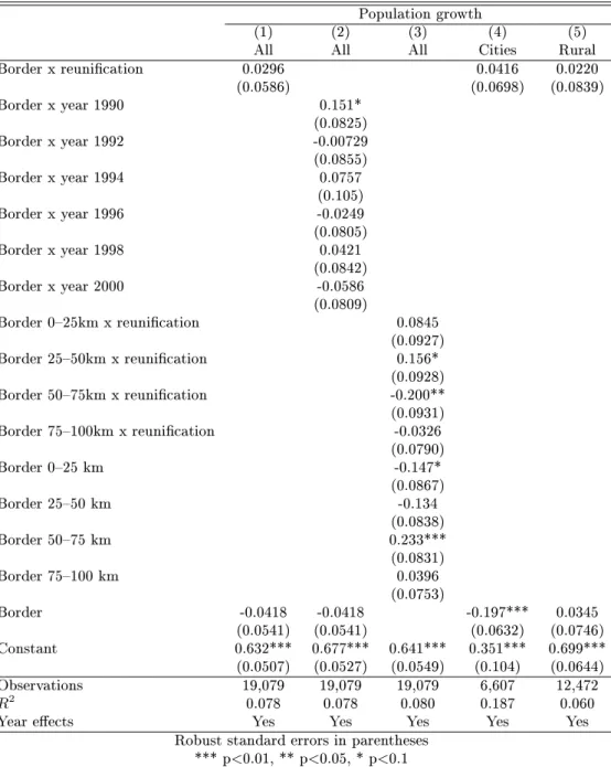
Redding and Sturm do not nd a signicant eect of reunication on population growth in the border area. They consider only cities. We replicate their baseline estimation here using population gures for all boroughs. The Helpman model detailed in the previous section predicts a larger eect on rural areas. Only including cities in their data, Redding and Sturm may have understated the eect of reunication. Table 1 shows the results of the baseline regressions.
We nd conrmation of their results. The interaction term of border area and reunication in column (1) is not signicant suggesting that the population growth is not systematically dierent in the border and the non-border area following reunication. The same applies to the border and year interactions in column (2), the time interactions do not produce a coherent picture.
In column (3) we split the border area into 25km pockets. Again no clear direction emerges, in particular as the only signicant coecient of the 5075km bracket sums to virtually zero when compared to the base coecient without time interaction. In columns (4) and (5) we divide the sample into cities and rural areas. The coecients of the border dummy suggest that cities within the border area experience a slower population growth than cities in the control group prior to reunication. But the same does not hold for rural areas.
Why do the Helpman model predictions dier from the actually observed population changes in the data? The possible explanations are related to the setup of the model. The key feature of the model is that its predictions concern the long run. Secondly, and similar to the division case, the long run equilibrium may not have been attained within a decade of reunication. Relocating from one area to another may take more than a few years. At the same time other variables in the model may adjust more quickly in the data. In particular the price of the non-traded amenity, which mainly captures the price of housing, may react more immediately as it entails expectations about the new long-run equilibrium spatial population distribution. The location of areas that were previously at the easternmost end of the Western world improved over night to the centre of Germany and Europe. This fundamental change in market access for these locations would, if the economic geography theory of market access and the Helpman model are correct, have to translate into higher population and higher price levels of the non-traded amenity.
But the long-run nature of these forces means that population gures may not be the most suitable variable when studying short-run eects. Ideally, one would nd leading indicators such as rm or consumer condence indices or granted construction permits. These do however not
Table 1: Baseline regressions population growth
Population growth
(1) (2) (3) (4) (5)
All All All Cities Rural
Border x reunication 0.0296 0.0416 0.0220
(0.0586) (0.0698) (0.0839)
Border x year 1990 0.151*
(0.0825)
Border x year 1992 -0.00729
(0.0855)
Border x year 1994 0.0757
(0.105)
Border x year 1996 -0.0249
(0.0805)
Border x year 1998 0.0421
(0.0842)
Border x year 2000 -0.0586
(0.0809)
Border 025km x reunication 0.0845
(0.0927)
Border 2550km x reunication 0.156*
(0.0928)
Border 5075km x reunication -0.200**
(0.0931)
Border 75100km x reunication -0.0326
(0.0790)
Border 025 km -0.147*
(0.0867)
Border 2550 km -0.134
(0.0838)
Border 5075 km 0.233***
(0.0831)
Border 75100 km 0.0396
(0.0753)
Border -0.0418 -0.0418 -0.197*** 0.0345
(0.0541) (0.0541) (0.0632) (0.0746)
Constant 0.632*** 0.677*** 0.641*** 0.351*** 0.699***
(0.0507) (0.0527) (0.0549) (0.104) (0.0644)
Observations 19,079 19,079 19,079 6,607 12,472
R2 0.078 0.078 0.080 0.187 0.060
Year eects Yes Yes Yes Yes Yes
Robust standard errors in parentheses
*** p<0.01, ** p<0.05, * p<0.1
exist on a disaggregate level such as boroughs and they are impossible to obtain backwards for the period 19802000.
Therefore, we put together a new data set on land values (Bodenrichtwerte). Prices of land react more quickly to market access shocks because they incorporate expectations about future demand stemming from a population relocation (Case and Shiller, 1989; Mankiw and Weil, 1989). Expectations about these future developments are realised more rapidly than actual rm and household moves. Using the asset pricing model for housing (Ayuso and Restoy, 2006) prices at time t = 0 entail all known information about future demand drivers. Hence when studying the short-run eects of the border opening, land values are a variable that serve as a leading indicator of a region's relative attractiveness. Ceteris paribus land prices are determined by demand and supply factors. With supply xed at least in the short-run, an improvement in market access leads to an expectation of rms locating to those regions triggering households to move in the future. This drives up demand and hence prices.
The empirical work has focused in particular on the nexus of land values and transport links.
Empirical studies have shown positive changes in land values following the announcement of infrastructure projects. For the US and Hong Kong studies show that price changes are factored into land values well before the completion of the corresponding infrastructure improvements (Yiu and Wong, 2005; Lai et al., 2007; Duncan, 2011). To take advantage of the price increases the Hong Kong government sold land in areas that were set to benet from the construction of a tunnel under the harbour to nance the construction of the project.
2.4 Model rearrangement
Of the seven equations that are simultaneously solved to compute general equilibrium we focus only on the one equation that relates the price of the non-tradeable amenity in our analysis we interpret this as the price of land PiH to total expenditure and the xed stock of the non-tradeable amenity.
PiH = (1−µ)Ei
Hi (2)
Rewriting PiH =BRWi, where BRW stands for Bodenrichtwerte or standard land values, and substituting in rst for total expenditueEiand then for the wagewiwe obtain the expression
BRWi = 1−µ
µ ξ[F M Ai]1/σ Li
Hi (3)
The housing supplyHiis treated as exogenously given and xed. Analogous to reinterpreting the price of the non-tradeable amenity as the value of land we dene the housing supply to be the area of a regioni. Then the fraction LHii is nothing but the population densityχi of a region.
In line with Redding and Sturm we can rearrange equation 3 as to arrive at equation 4
log(χi) = α +βi log(M Ai) +log(BRWi) + i (4) which relates the population density of location iat timetto the regions market access and its land value. This specication is used by Redding and Sturm and will be our rst reference point in the analysis of our data set.
We simplify further and use only one measure of market access combining rm and consumer market access. German reunication is a shock to market access and this shock is dierent in magnitude depending on a region's proximity to the inner German border. The model is a static model predicting long-run equilibrium outcomes, but we can look at rst dierences taking partial derivatives. In order to theoretically understand the implications of the model we thus compute the marginal change in land values with respect to a change in market access and obtain
∂BRWi
∂M Ai = 1−µ µ
∂
∂M Ai [M Ai]1/σ χi (5) which captures the rst-round eect of a change in market access. Taking the logarithm yields a linear equation that is empirically tractable
Growth BRWi,t = α +βi,t Growth(M arket P otential)i
+controlsi,t+ i
(6)
where growth rates are annualised rst dierences of a variable, α is a constant and β the coecient of interest.
To derive the theoretical long-run equilibrium eect through the feedback eect in the system of simultaneous equations a simulation using a software programme such as MATLAB is required.
The testable predictions are summarised at the beginning of section 4.
3 Data
3.1 Standard land values
Germany with its sixteen states is a federation and accordingly each federal state consists of administrative districts. Each district in turn keeps its own expert committee (Gutachterauss- chuss) which collects the notarial records of land transactions in their district. On the basis of these market transactions the expert committees set a standard land value expressed as a per square meter price for every borough in their district. A more detailed account on the nature of the expert committees can be found in Kleiber, Simon, and Weyers (2007). The standard land values are hence based on current market values (Verkehrswerte). The standard land value is the reference value for the sale of public property, the taxation of land or the calculation of inheritance tax. The standard land values are computed every two years. The expert commit- tees consist of a chairperson and independent experts from backgrounds such as construction, architecture or engineering.
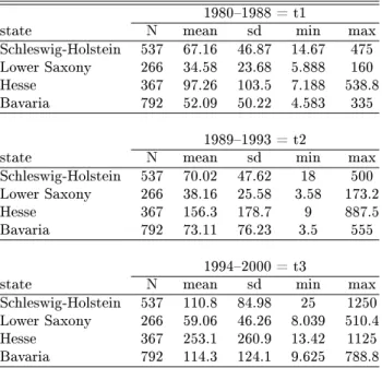
In Lower Saxony a central expert committee provided the relevant land values. In Schleswig- Holstein, Hesse and Bavaria each expert committee was contacted individually. For data pro- tection reasons the data on individual transaction purchasing prices were not attainable. In- stead the expert committees determine the land values on the basis of all transaction records from the previous two year interval. We digitised the obtained paper copies. In the pres- ence of several land values per borough per year we computed the median value. To obtain a fully balanced sample the period 19802000 was divided into three subperiods. The rst period t1 (01.01.198031.12.1988), the second period t2 (01.01.198931.12.1992), and period t3 (01.01.199331.12.2000).
Table 2 presents descriptive statistics of standard land values grouped by state and time period: the number of observations, the mean, the standard deviation, and the minimum and maximum values. The complete and fully balanced data set spans 11 year observations and consists of 1,533 individual municipalities including 545 cities, i.e. regions with a population larger 5,000 and 988 rural boroughs with a population smaller 5,000.
The dierences in mean land values across space can be attributed to dierent population densities. Lower Saxony as the least densely populated state has the lowest mean standard land values across all boroughs. Hesse as the most densely populated state has the highest levels.
The vast dierences in mean levels can in part also be attributed to the dierent structure of
Table 2: Standard land values
19801988 = t1
state N mean sd min max
Schleswig-Holstein 537 67.16 46.87 14.67 475 Lower Saxony 266 34.58 23.68 5.888 160
Hesse 367 97.26 103.5 7.188 538.8
Bavaria 792 52.09 50.22 4.583 335
19891993 = t2
state N mean sd min max
Schleswig-Holstein 537 70.02 47.62 18 500 Lower Saxony 266 38.16 25.58 3.58 173.2
Hesse 367 156.3 178.7 9 887.5
Bavaria 792 73.11 76.23 3.5 555
19942000 = t3
state N mean sd min max
Schleswig-Holstein 537 110.8 84.98 25 1250 Lower Saxony 266 59.06 46.26 8.039 510.4
Hesse 367 253.1 260.9 13.42 1125
Bavaria 792 114.3 124.1 9.625 788.8
the states. Frankfurt is the largest city in our sample and in particular the neighbouring areas exhibit above-mean standard land values. On the other hand we only consider the four most Northern Bavarian administrative districts thereby excluding Munich and its urban hinterland.
Hamburg is not part of the sample either.
3.2 Market potential / market access
We interpret the shock from reunication as a positive shock to market access. Accord- ingly we disaggregate a region's market potential into three parts. Its own market potential (market potential eigeni,t), the market potential located in West Germany and market poten- tial associated with East German districts.
M arket P otentiali,t =M P eigeni,t+M P westi,t+M P easti,t (7) We choose an alternative approach to Helpman which is similiar to Donaldson and Hornbeck (2016) who employ a more general concept of market access that does not distinguish between rm and consumer market access. Market potentials are computed on the borough level which for the considered states in West Germany includes all 1,533 West German boroughs. Market potential in district i is the sum of its own market potential and foreign market potential.
The early theoretical concept of market access dates back to Harris (1954) while a more recent contribution applying a market access function to a Krugman model of economic geography can
be found in Hanson (2005). The own market potential is computed as boroughs' i population divided by the distance to the centre of the borough. Likewise foreign market potential is the sum of all other district's population gures weighted by their distance from the centre of district j to the centre of borough i.
M arket P otentiali = P
i
P opulationi
Distancei
+ P
j
P opulationj
Distanceij (8)
Population gures are taken from the regional database of the German states (Statistische Aemter des Bundes und der Laender (2000)). Distances to the district centre are computed assuming a circle shape of the district. The formula 0.376×(areai)1/2 (Head and Mayer, 2000) is used to derive the average distance to the geographic centre of a district.
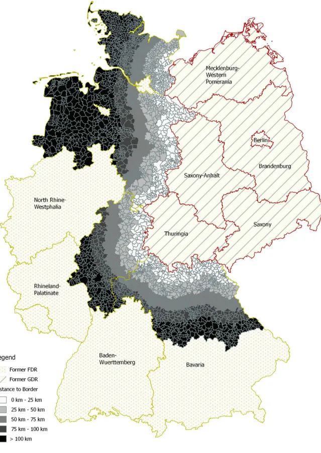
An alternative approach is to use actual travel times. The data in Nitsch and Wolf (2013) are based on actual travel times between transport districts (Verkehrsbezirke). The drawback of this method in the present study is the shape of the transport districts. We are interested in the eect of reunication conditional on distance to the inner German border. But some transport districts do stretch from boroughs directly adjacent to the border up to 100km inland.
Figure 3 depicts distances to the inner German border for West German boroughs.
3.3 Geography and time
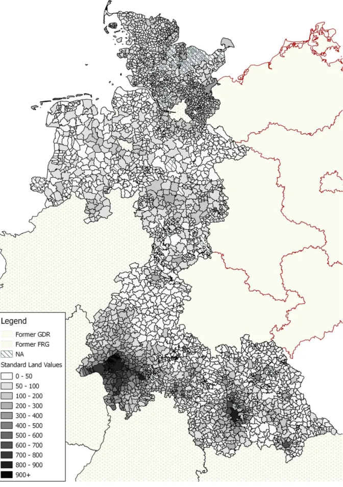
Figure 4 maps standard land values in the four German states Schleswig-Holstein, Lower Saxony, Hesse and Bavaria in the year 2000. The map illustrates the relatively low levels of land values along the former inner-German border. Additionally, agglomerations such as Hanover, Frankfurt or Nuremberg are clearly visible with higher land values and with a spatial eect on the neighbouring regions. Bremen and Hamburg themselves are not part of the sample, but the knock-on eect on the urban commuting regions in Schleswig-Holstein and Lower Saxony is visible.
One potential concern of the data is the heterogeneity across expert committees and across federal states. But for the econometric analysis in section 4 this problem can be tackled by including district xed eects to control for potentially inconsistent land value computation by expert committees. The inclusion of xed eects remedies the problem if we assume that expert committees did not alter their valuation methods systematically over time. We argue that this is a reasonable assumption given the size of the expert committees and their stability over time.
Figure 3: Distances to inner German border
Figure 4: Standard land values in West Germany, 2000
Throughout the empirical section we use annualised growth rates for standard land values and the market potential measure.
In order to test for the eect of reunication we dene the dummy:
reunif ication=
0 if year∈[1980;1988]
1 if year∈[1989;2000]
(9)
The date of the border opening on 9th November 1989 allows us to identify the reunication shock precisely. As land values are reported every two years the last year in the pre-reunication period 1988 captures the period 1st January 1987 to 31st December 1988. Reunication falls in the period of the 1990 observation spanning 1st January 1989 to 31st December 1990.
4 Empirical results
The empirical analysis consists of four steps. At rst we run a panel analysis regression of the change in land values on a set of distance and time dummies. Finding a signicant eect of reunication on land value growth rates with a dierence in cities and rural boroughs, we then compare the Helpman model predictions with the observed land and population growth rates. Land values have adjusted more quickly than population levels. We deconstruct the market access variation into its three components and consider the relative as well as the absolut intensity of the market access shock. The absolute size of the market access shock stemming from the opening of the border conrms the baseline regression results, but the relative shock analysis conrms the dierent eects across boroughs. The last subsection of the main results section looks at the within-border variation. We conrm that smaller regions do indeed exhibit a larger response to the reunication shock than larger boroughs. It required however an initial population level to take advantage of the market access shock.
The robustness checks rst establish the plausibility of the relationship in the Helpman model between land values, population and market access. The section adds to the empirical ndings using distance to local markets, manufacturing employment shares and a study of the border periphery subsidy to underline the main empirical ndings.
Redding and Sturm analyse the shock that German division after WWII had on city size.
They nd evidence that cities closer to the inner German border were more aected and that this eect diminished over time. In addition they only nd a negligible eect of reunication.
In their study Redding and Sturm focus on cities with a population of 20,000 and above.
With the inclusion of all rural areas we analyse the development of land prices (Boden- richtwerte) from 1980 until 2000 as one indicator for economic activity. This allows us to condition on a starting point that goes beyond a simple small city/ large city dierentiation.
We match these land values with other data on population, market potential and housing stock.
We follow Redding and Sturm in assuming that a stable long-run equilibrium was attained after a 45-years adjustment process starting after division in 1945.
We have derived three empirical predictions that we will proceed to test in this section 4 using our data. For the price of the non-traded amenity (i.e. the value of land) these are the analogous predictions to the population levels. They are as follows
1. The value of land in locationiis positively related to the location's characteristics such as market access and population density.
2. A (positive) shock to market access results in a (positive) change in the value of land all other things equal.
3. The market acces shock from reunication aected boroughs with a smaller population more strongly.
4.1 Baseline results
Figures 5 and 6 visualise the dierent land price developments in the border and non-border boroughs. In gure 5 the standard land value growth index is displayed where the year 1990 is indexed at 1. The indices are computed dividing the respective annual growth rates by the average rate of change in the pre-reunication period. When comparing the two indices we notice a break around 1990, the year of reunication. The two indices developed similarly before 1990 and indeed only exhibited a small upward trend, but this upward trend accelerates after 1990.
In particular the rst four years until 1994 are characterised by higher growth rates, but this increase in growth rates slows down between 1994 and 2000 for both groups, the border and the non-border group. This suggestive evidence will be explored in more detail. The average borough in the sample includes both cities and rural areas and averaging over the two groups may cloud dierent responses to reunication.
Figure 6 displays the dierence between the two indices. Corresponding to the previous gure the dierence is around zero until 1990 when the dierence starts widening. From 1994
.9511.051.11.151.2
Index (1990=1)
1980 1982 1984 1986 1988 1990 1992 1994 1996 1998 2000 Year
Border Boroughs Non-border Boroughs
Border vs. Non-Border Growth Index
Figure 5: Border vs. Non-Border growth index
0.05.1.15
Border Group - Non-border Group
1980 1982 1984 1986 1988 1990 1992 1994 1996 1998 2000 Difference in Land Price Growth Indices, Border - Non-border
Figure 6: Dierence border - non-border index
onwards the gap widens more slowly until 2000. At the end of the sample period in the year 2000 the dierence between border and the non-border land value index is around 12%.
We now turn to the baseline regression equation which is restated below:
Growth BRWi,t = βi,t(Reunif ication X Border) +γi,tBorder +controlsi,t+ i,t
(10)
Table 3 summarises the baseline regression results obtained from three samples. Columns (1) (3) in table 3 display results for the full sample, columns (4)(6) consider only cities (popu- lation>5,000), and columns (7)(9) capture results including only boroughs with a population smaller 5,000. In all three samples three specication are run.
Regressions (1), (4) and (7) estimate the interaction eect of the reunication period with the border area. For the full sample we nd a signicant positive eect of reunication in the border area compared to the boroughs outside the treatment border region. Considering the eect for cities and rural areas separately yields a dierent picture. The eect is even larger for rural regions (column 9), but the eect is negative for cities although not signicant. That is to say that the land value development of cities in the border region cannot be distinguished from the development in cities in the control group.
Columns (2), (5) and (8) display results when the reunication time dummy is split into yearly dummies. Again the coecients of interest are the interaction coecients of the border dummies and the time dummies. Regarding the results of the full sample it appears surprising that the only signicant eect occurred in the year 2000. The other coecients are with the ex- ception of 1994 positive, but not signicant. The reason for this nding becomes apparent when considering the split samples. Column (5) suggests that cities in the border area experienced a signicant decline in land values in the years 1992 and 1996, but annualised growth rates are positive in the two years around 1998. The other year-border interactions are not signicant.
For rural boroughs the almost opposite eect emerges: larger and signicant growth rates are found for four out of six year-border interactions. Overall the size of the coecients declines from 1992 onwards turning even negative for 1998, albeit at a lower level of signicance.
Lastly, regressions (3), (6) and (9) split up the border dummy into four 25km groups. Column (3) suggests that the eect of reunication was strongest for the treatment group in the 2550km bin, and still positive signicant for the 5075km group at a lower level. The coecients for the 025km and 75100km are positive, but cannot be signicantly distinguished from zero.
Separating again the city from the rural sample we nd that the eect for the city only sample is signicantly negative for cities in the immediate border vicinity in the 025km group. The other eects are insignicant. The rural sample yields a markedly dierent picture. The positive eect of reunication on land value growth rates is strongest in the 025km and 2550km group.
It then declines, but remains signicantly positive in the other border treatment groups.
It has been shown that cities and rural boroughs exhibit a very dierent reaction to the reunication shock. The choice of the sample matters. Comparing cities within the border region only to cities outside the border region and likewise rural boroughs only to other rural boroughs one may neglect important features of the data hidden in the cross comparison. For that reason appendix 6 contains baseline regressions with an additional interaction variable of Border X Reunif ication X City. But the results do not yield any new insights.
The next section therefore presents a direct comparison of total cumulative land value changes in rural and city boroughs split into border and non-border boroughs. We compare this to the Helpman model predictions.
4.2 Prediction vs. realisation
Figures 7 and 8 summarise the key results from this paper. Land prices have within a decade already realised the predicted gains, but population growth has not seen the same trajectory.
Land values appear to adjust more rapidly, but population levels do not.
Both gures compare predicted and in the data observed cumulative total changes in rural boroughs (gure 7) and cities (gure 8) both in terms of population growth and land value growth. Within these gures we then divide them up again into non-border boroughs and border boroughs. In total these two gures comprise sixteen aggregate data points.
Beginning with the left panel in gure 7 we observe that the model predicts a very similar long-run total growth of population and land prices. The border area is predicted to do relatively better than the non-border area. The magnitude of the predicted growth is now contrasted with the actually observed changes up until 2000. The model predicts an increase in population and land values in the non-border area of around 5%, but the data tell a dierent story. We measure a population decline of 6%. Despite this fall in population the land values increase by around 12%, markedly above the predicted change. The same applies to the border area.
Population has grown an average of 2%, but the model predicts a long-run growth of 17%. At the same time land values have overshot their predicted total growth by 7% within a decade. We
Table3:Reunicationbaseline Landvaluegrowth (1)(2)(3)(4)(5)(6)(7)(8)(9) AllAllAllCitiesCitiesCitiesRuralRuralRural Borderxreunication0.993***-0.5131.603*** (0.361)(0.651)(0.444) Borderxyear19901.102-0.4132.336*** (0.696)(1.502)(0.764) Borderxyear19920.931-3.754**3.835*** (0.722)(1.495)(0.789) Borderxyear1994-0.494-1.7970.274 (0.651)(1.189)(0.791) Borderxyear19960.974-3.327**2.771*** (0.812)(1.539)(0.958) Borderxyear19981.4256.012***-2.477* (0.965)(1.692)(1.271) Borderxyear20002.045***0.2682.472*** (0.548)(0.889)(0.713) Border025kmxreunication0.762-3.910***2.679*** (0.533)(1.148)(0.597) Border2550kmxreunication2.612***1.4753.291*** (0.591)(0.925)(0.770) Border5075kmxreunication1.022*-0.3301.842*** (0.538)(0.933)(0.661) Border75100kmxreunication0.716-1.1211.938*** (0.510)(0.791)(0.663) Border025km-2.146***0.315-3.182*** (0.401)(0.918)(0.433) Border2550km-1.615***-0.331-2.180*** (0.426)(0.730)(0.527) Border5075km-1.023**0.0396-1.471*** (0.428)(0.736)(0.522) Border75100km-0.952**0.306-1.713*** (0.386)(0.654)(0.477) Border-1.188***-1.188***-0.0991-0.107-1.528***-1.525*** (0.272)(0.272)(0.510)(0.510)(0.327)(0.328) Constant0.419-0.1140.576*-1.280***-1.550***-1.038*1.015***0.5360.957** (0.274)(0.335)(0.300)(0.494)(0.521)(0.530)(0.339)(0.463)(0.376) Observations16,86316,86316,8635,9955,9955,99510,86810,86810,868 R20.0360.0360.0380.0420.0500.0470.0390.0430.041 YeareectsYesYesYesYesYesYesYesYesYes Robuststandarderrorsinparentheses ***p<0.01,**p<0.05,*p<0.1
attribute this to the evidence that prices do react much more quickly to the market access shock of reunication. They incorporate expectations about future (predicted) population movements and preempt the then induced changes to land values. In particular, the border area population has grown only a tiny bit of the predicted way, but land prices have even overshot the model predictions. The in the data observed negative population growth in the non-border area may be driven by an underlying urbanisation trend, a trend which does not feature in the Helpman model.
Figure 7: Rural borough growth
-100102030
Non-border Border Non-border Border
Simulation Observation
Population growth Land value growth
Percentage change
Graphs by Simulation vs Observation
Turning now to the simulation panel in gure 8, city growth in the non-border was predicted to be -5% for population and land value levels. The border area cities were on average predicted to grow by 12%, and land values were predicted to go up by 16%. Again the observed growth rates paint another picture. Cities in the border and the non-border area have grown, but the non-border cities grew by an extra 3% on average. Land values in the non-border have gone up in similar magnitude to the population levels. But in the border area land values have outpaced population growth again. Population has grown only about a third of the expected way, but
land prices have already adjusted 80% to the predicted level.
Apart from the information content explanation, the comparison with the rural areas may potentially hint at quicker population relocations in cities. Opposed to rural areas where ad- justments happen over a longer time frame, cities react more quickly.
Figure 8: City growth
-5051015
Non-border Border Non-border Border
Simulation Observation
Population growth Land value growth
Percentage change
Graphs by Simulation vs Observation
In sum, we have found conrmation of the Helpman model predictions. First, regions in the immediate border area do relatively better than the control group outside 100km of the border.
Furthermore, regions with a smaller population are relatively more aected by the market access shock as their own market potential is small compared to the added market potential.
4.3 Shock intensity
In addition to the dierence-in-dierences analysis presented in previous subsections the reunication shock allows for an analysis that does not clearly distinguish between a treatment and a control group. This is particularly important as one might be concerned about the choice of treatment and control groups in the previous subsections.
Instead the whole sample is divided up into quintiles and assigned values 15. These quintiles measure two dierent types of shock intensity. The rst one is relative shock intensity. 20% of the boroughs that experienced relatively the smallest shock are in the rst quintile (Q1). Q2 then captures the 2040% quintiles, and so forth. This measure of shock intensity is interacted with the reunication time dummy. The relative shock intensity may be challenged on the grounds that one cannot disentangle the eects caused by closer distance from the ones from a larger population.
The second measure is absolute shock intensity. This is in some ways another way to measure distance to border, but again we do not assign a clear control group. We consider two measures of the market access shock, one in absolute terms and the other in relative terms.
The coecients of interest in columns (1)(3) of table 4 are the interactions of the reunica- tion time dummy with the relative market access shock quintiles. Considering all three dierent samples it emerges that the middle quintile interaction is always negative, even if not always signicant. At the same time all other interactions are positive and apart from the city sample (where only the interaction of the rst quintile is signicant at 5%) all signicant. We interpret this as follows: regions that received a medium intensity treatment of the market access shock be that due to their relative size or their medium distance to the border show the smallest reaction. All other regions exhibit a larger treatment eect which in the full sample and the rural sample specication is largest for the quintile that is relatively most aected.
It is again important to note that one cannot pinpoint at either distance or population measure to cause the quintile anity of boroughs. Therefore, we now consider absolute shock intensity which is another way of measuring the border distance. Here boroughs in the immediate border vicinity were in absolute terms hit hardest by the reunication treatment. The advantage over the baseline specication is that there is no treatment or control group, but rather one continuous treatment group. This addresses concerns about the choice of the treatment group.
The results are displayed in columns (4)(6). Simplifying the results one can say that the boroughs in the lowest quintile, i.e. boroughs that received the smallest absolute market access shock, did experience a negative land value growth in the reunication period. The coecients then increase in magnitude (albeit not strictly monotonically) and are largest for the quintile that received the largest absolute shock. The coecients are signicant at the 1% level with the exception of the 2nd4th quintile interactions in the city sample.
Overall these results conrm our ndings of the baseline border specication.
Table4:Shockintensity Landvaluegrowth (1)(2)(3)(4)(5)(6) AllCitiesRuralAllCitiesRural ReunicationxrelativeshockQ11.654***1.431**1.747** (0.464)(0.694)(0.768) ReunicationxrelativeshockQ21.693***0.7312.036*** (0.398)(0.677)(0.501) ReunicationxrelativeshockQ3-0.726*-0.658-0.935** (0.386)(0.736)(0.450) ReunicationxrelativeshockQ41.664***1.0312.125*** (0.393)(0.780)(0.464) ReunicationxrelativeshockQ53.350***0.5414.246*** (0.422)(0.871)(0.488) ReunicationxabsoluteshockQ1-1.810***-2.528***-1.250** (0.454)(0.905)(0.518) ReunicationxabsoluteshockQ21.741***0.7322.171*** (0.369)(0.670)(0.459) ReunicationxabsoluteshockQ31.323***1.0151.323*** (0.373)(0.643)(0.465) ReunicationxabsoluteshockQ42.324***1.427*2.727*** (0.410)(0.797)(0.474) ReunicationxabsoluteshockQ55.132***2.700***6.260*** (0.460)(0.887)(0.534) Relativeshockintensity-0.597***-0.266-0.712*** (0.120)(0.214)(0.153) Absoluteshockintensity-1.585***-1.357***-1.666*** (0.105)(0.234)(0.112) Constant0.719-1.1891.348**5.240***4.973***5.285*** (0.544)(0.973)(0.680)(0.382)(0.816)(0.408) Observations16,8635,99510,86816,8635,99510,868 R2 0.0410.0450.0480.0380.0410.045 YeareectsYesYesYesYesYesYes Robuststandarderrorsinparentheses ***p<0.01,**p<0.05,*p<0.1
4.4 The importance of size
After establishing a reunication treatment eect, which was stronger for the rural boroughs than for cities, we now turn to the dierent magnitudes of this eect. We nd severe within rural borough variation of land value growth in the border group. The same applies to within city variation. Purely distinguishing between city and rural clouds this interesting feature of the data. The last gure in the subsection therefore splits the border area itself up into population deciles. The number of boroughs in each decile is the same. Figure 9 documents mean cumulative growth which was largest in boroughs in the 2nd3rd population decile. After this decile the cumulative land price growth declines monotonically with a slight increase again at the 10th decile.
We interpret this as evidence that boroughs with a smaller population exhibit indeed a larger mean cumulative land value gain, but it required an initial level of population to benet from the reunication shock in the same way as the 3rd decile. This can be seen as the rst decile increased on average over the ten years by around 27 percent when the third decile gained an average of almost 40%. The boroughs in the third decile are relatively sparsely populated with the mean population of the third decile population 1,292.
Boroughs in the sixth decile have a mean population of 5,762 and fall in the small city category. The mean cumulative land value growth is around 27% and continues to decline further.
The decile with the lowest land value growth has an average population of 12,115 inhabitants, again falling into the small city category. The 10th decile with an average population of 32,982 (and thereby a medium city) shows an average increase in land values of around 18%, somewhat higher than the 9th decile but still markedly below the border group average gain.
To sum up not only does the distinction between city / non-city and border / non-border matter, even within the border treatment group there exists heterogeneity in the land value responses to reunication.
5 Robustness checks
This section presents a number of robustness checks beginning with a plausibility check of the data in the pre-reunication period. We explore other potential drivers of land value responses such as distance to local markets, employment shares in the tradeables sector and the border periphery subsidy.
Figure 9: Growth of land prices by population deciles
5.1 Cross-section analysis
The previous sections rest on the assumption that the theoretical relationship between the land value data, the population gures and the market access variables is indeed empirically plausible. The descriptive evidence presented earlier suggest that the data match features of the observed world, but in addition we run here cross-section regressions to back up this suggestive evidence.
We begin by testing prediction 1 of the Helpman model, the relationship between popula- tion, market access and land values. We restate equation 4 for convenience and estimate three specications
BRWi=β Xi+ controlsi+ i (11) where Xi is replaced by population size, border groups or market potential measures de- pending on the specication.
The results for the estimation of the equations are displayed in table 5. Column (1) of table 5 conrms the signicant eect of population levels on land values. We obtain a similar result when considering population density instead of population levels. Indeed population levels and market potential are highly signicant determinants of standard land values. Likewise distance to border has a negative eect on land value levels with a declining eect in the 25km intervals.
Boroughs within a 25km perimeter of the inner German border exhibit on average standard land values that are 47.43 DM lower per square meter than land values in the control group (boroughs that are at least 100km away from the border). Likewise boroughs in the 2550km distance group from the border have land values that are on average 36.94 DM lower. The 5075km group is not signicantly dierent from the control group. The same applies to the 75100km group which is not displayed here.
Turning to columns (3) and (4) we consider the correlation between market potential and land values. Column (3) conrms a highly signicant correlation between the two. Disentangling the contribution of a borough's own market potential and foreign market potential it becomes apparent that a borough's own market potential has a far larger eect on land values than the foreign market potential. This holds however only in the steady pre-reunication equilibrium.
As shown earlier the opening of the border translated into a multiplication of market potential of up to 15-times for some boroughs. The change in market potential comes almost entirely from the change in foreign market potential.
Table 5: Cross-section pre-reunication Land value level
(1) (2) (3) (4)
All All All All
Population (in 10,000) 11.61***
(2.249)
Border 025 km -47.43***
(3.593)
Border 2550 km -36.94***
(4.804)
Border 5075 km -2.386
(5.332)
Market Potential 9.600***
(0.627)
Own Market Potential 41.66***
(2.677)
Foreign Market Potential 3.183***
(0.651)
Constant 89.73*** 114.4*** -109.8*** -23.33*
(2.844) (3.743) (14.38) (13.45)
Observations 9,810 9,810 9,810 9,810
R2 0.196 0.153 0.201 0.357
Year eects No No No No
Robust standard errors in parentheses
*** p<0.01, ** p<0.05, * p<0.1 5.2 Distance to local markets
A further concern might be that growth in land prices is driven by proximity to local markets instead of markets further away. The change in market potential coming from a change in the immediate markets may have a larger eect on a borough's land value than a (potentially) larger change further away with missing infrastructure links. Rural areas near cities may have benetted from their close location to larger markets, thereby being able to take advantage of export opportunities or shorter commuting times.
We test this by including the share of employment in the manufacturing sector as an in- strument for capacity to benet from a market access increase. The share of manufacturing employment is measured as the total number of people employed in the manufacturing sector divided by total population. It is of course an imperfect measure of actual employment shares as one should divide the number of manufacturing employees by the labour force instead of total population. For the considered period we were unable to obtain labour force gures on a disaggregate borough level. As employment gures are only available on a municipality level,