ORIGINAL PAPER
Exploring the determinants of real estate liquidity from an alternative perspective: censored quantile regression in real estate research
Marcelo Cajias1 · Philipp Freudenreich2 · Anna Freudenreich2
Published online: 3 June 2020
© The Author(s) 2020
Abstract
In this paper, the liquidity (inverse of time on market) of rental dwellings and its determinants for different liquidity quantiles are examined for the seven largest Ger- man cities. The determinants are estimated using censored quantile regressions in order to investigate the impact on very liquid to very illiquid dwellings. As market heterogeneity is not only observed between cities but also within a city, each of the seven cities is considered individually. Micro data for almost 500,000 observations from 2013 to 2017 is used to examine the time on market. Substantial differences in the magnitude and direction of the regression coefficients for the different liquidity quantiles are found. Furthermore, both the magnitude and direction of the impact of an explanatory variable on the liquidity, differ between the cities. To the best of the authors’ knowledge this is the first paper, to apply censored quantile regressions to liquidity analysis of the real estate rental market. The model reveals that the pro- portionality assumption underlying the Cox proportional hazards model cannot be confirmed for all variables across all cities, but for most of them.
Keywords Residential · Housing · Liquidity · Censored quantile regression · Time on market
Electronic supplementary material The online version of this article (https ://doi.org/10.1007/s1157 3-020-00988 -w) contains supplementary material, which is available to authorized users.
* Philipp Freudenreich philipp.freudenreich@irebs.de
Marcelo Cajias
marcelo.cajias@patrizia.ag Anna Freudenreich anna.freudenreich@irebs.de
1 Patrizia Immobilien AG, Fuggerstrasse 26, 86150 Augsburg, Germany
2 International Real Estate Business School, University of Regensburg, Universitaetsstrasse 31, 93053 Regensburg, Germany
JEL Classification C31 · C34 · R21 · R32
1 Introduction
The concept of asset liquidity in the residential rental market is somewhat blurred.
In the investment market, asset liquidity traditionally measures the time it takes the owner to turn an asset into cash. In the rental market on the other hand, asset liquid- ity measures the time it takes the landlord to find a new tenant, i.e. from introduc- ing the dwelling to the market until the signing of the rental contract. In this paper, liquidity is defined as the inverse of the time on market (TOM) of rental dwellings, i.e. the higher the time on market, the lower the liquidity.1 Whether the letting pro- cess is quick or slow, depends mainly, on the initial asking rent, the structural qual- ity and location of the asset, demand for space, and the overall market conditions. A detailed understanding of these major drivers of marketing time of rental dwellings is the objective of this paper. To extract more insightful information from the avail- able data, the study introduces a modelling technique which is new to the field and uses the results to validate the outcome of the most established approach to measure liquidity, which is the Cox (1972) proportional hazards model (PHM).
This paper focuses on the residential rental markets of the seven largest Ger- man cities (descending order by population): Berlin, Hamburg, Munich, Cologne, Frankfurt, Stuttgart, and Dusseldorf. While for the methodological aim of the paper, these markets are subsidiary, it is useful to understand the German rental regula- tory framework and gain some insights into the housing markets in order to follow the contextual aim of this specific study. By law, tenants in Germany usually have a 3 months cancelation period, for which reason a dwelling is typically brought onto the market before the tenant leaves.2 With a national ownership rate of roughly 43%
as of 2013, the first year of the sample period, clearly more than half of German households rent their homes and hence the rental market deserves closer attention.
Voigtländer (2009), Bentzien et al. (2012), Lerbs and Oberst (2014), and Reisen- bichler (2016) explain in detail the reasons for this distinctive market feature. The considered cities exhibit ownership rates that are far lower than the German average, ranging from 33% in Stuttgart to 16% in Berlin. Therefore, especially in these cit- ies, the rental market plays a significant role. While six of the cities can be general- ized as long-established markets, Berlin shows stronger growth rates in population, purchasing power, employment, rents and purchase prices for real estate, however, starting from lower absolute values in those figures. For decades, the western Ger- man cities have developed into trans-regional hubs for education and employment.
Berlin has “only” been able to benefit from the nationwide improvement after the reunification of Germany in 1990, however, since then its positive development was substantial.
1 Based on the definition of Wood and Wood (1985).
2 Landlords can only terminate the contract to use the dwelling for themselves or for other household members.
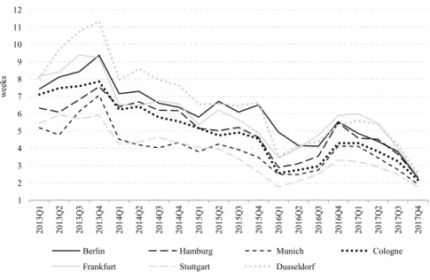
Figure 1 illustrates the average time on market for the seven largest German cit- ies extracted from the underlying dataset. Despite some up and down movements, the graph clearly shows a continuous decline in time on market within the last years. This development points to an increasingly strong demand on the rental mar- ket, as prospective tenants have to shorten their decision-making process because of high competition for an insufficient supply. This excess demand was recognized by Held and Waltersbacher (2015) who claimed that this comprises 272,000 newly constructed dwellings per year on a national level for the years 2015–2020, while the actual completion did not satisfy this demand.3 In addition, the use of online platforms might lead to better informed market participants, resulting in a narrower price assessment and hence less market uncertainty and increased market efficiency.
Since the aim of this paper is to understand the drivers of demand for rental space by means of a well-established method and the introduction of a method new to the field of real estate, the first step is to explore time on market via the Cox PHM.
Next, an advanced econometric approach is introduced. To the best of the authors’
knowledge this study is the first, to investigate the determinants of time on market by applying a censored quantile regression (CQR) in real estate research. The CQR aims to explain the variation of time on market as a function of dwelling charac- teristics and other spatial and socioeconomic characteristics. The decisive feature
1 2 3 4 5 6 7 8 9 10 11 12
2013Q1 2013Q2 2013Q3 2013Q4 2014Q1 2014Q2 2014Q3 2014Q4 2015Q1 2015Q2 2015Q3 2015Q4 2016Q1 2016Q2 2016Q3 2016Q4 2017Q1 2017Q2 2017Q3 2017Q4
Berlin Hamburg Munich Cologne
Frankfurt Stuttgart Dusseldorf
weeks
Fig. 1 Average time on market in weeks in the seven largest German cities. This figure displays the aver- age time on market in weeks in the seven largest German cities from 2013 Q1 to 2017 Q4. The data con- sists of 482,196 observations of the residential rental market
3 According to the Federal Statistical Office (2018) dwelling completion was: 216,727 (2015), 235,658 (2016) and 245,304 (2017).
of the analysis is that CQRs are used to model any quantile of the distribution of the dependent variable. Chaudhuri et al. (1997) stress this feature as a great advan- tage compared to mean regressions, as distributions might not only be different in terms of their means but might differ especially in their upper and lower tails. CQRs can quantify the impact of a covariate on the dependent variable for any quantile, compared to only the center of the population. The CQR, as an expansion of the survival regression analysis, is expected to yield more accurate estimations and to provide a more complete statistical analysis for understanding the factors driving liquidity and the underlying demand. The dataset consists of 482,196 observations on the rental markets of the seven largest German cities between 2013 Q1 and 2017 Q4. The study reveals that the magnitude and direction of impact of an explana- tory variable on time on market differs between the cities. Hence, this implies the importance of analyzing each city individually and not the seven cities or even the German market as whole. Furthermore, the magnitude and direction of effect of an explanatory variable on the liquidity of a dwelling exhibits differences between time on market quantiles within a city. This implies that, the proportional hazards assumption, underlying the Cox PHM is violated for individual explanatory vari- ables and cities and thus emphasizes the use of the CQR approach for the time on market analysis. The study concludes that the heterogeneity across the liquidity quantiles, as well as the heterogeneity between the cities, are accountable for the dis- tinguishable impacts of changes in the covariates on time on market. These findings should of course be of interest to current and future landlords, as they reveal both the characteristics of dwellings along the liquidity distribution (e.g. the existence of built-in kitchen), as well as the impact of a change in characteristics on the liquid- ity of dwellings (e.g. impact of installing a built-in kitchen). Therefore, landlords should be able to infer whether a dwelling displays the characteristics of a highly liquid thus highly demanded dwelling, or what actions they could take in order to increase the expected liquidity, e.g. install a built-in kitchen or change the floor plan to increase the number of rooms. Furthermore, the findings suggest that nationwide or even statewide policy measures might not be expedient to address the specific situation on the residential rental real estate market of a particular region, city or neighborhood.
The remainder of this paper proceeds as follows: The next Section provides a lit- erature review. Section 3 describes the underlying econometric model, followed by a detailed description of the dataset and the descriptive statistics in Sect. 4. Estimation results are presented and discussed in Sect. 5. Section 6 concludes.
2 Literature review
Belkin et al. (1976) conducted one of the first empirical studies analyzing real estate liquidity for different market segments. They divide the market according to geographic areas, price segments and buyers’ search space. By doing so, they analyze the relationship between time on market and the spread between list- ing price and selling price, using ordinary least squares (OLS) estimation tech- niques. They find essential differences between market segments. Especially in
high-price segments, deviations from the initial list price had a more pronounced effect on time on market. The determinants of time on market considering differ- ent price segments have comprehensively been analyzed in the literature. Kang and Gardner (1989) found that the impacts on time on market do vary in magni- tude between low-, medium-, and high-price segments. While Kang and Gardner (1989) did not identify the simultaneity problem between time on market and the selling price, Yavas and Yang (1995) applied a two-stage least squares (2SLS) estimation to deal with the fact that time on market and price mutually influence each other. They exhibit a significant positive impact of price on time on market in the medium-price segment, whereas this effect is insignificant for houses in the low- and high-price segments. Allen et al. (2009) also use a multi-step pro- cedure to analyze the relationship between asking rent and time on market in the rental market for single-family residential rental listings. Based on asking rents, the sample is divided into three price segments. They find that underpricing of asking rents and time on market move in the same direction in all price segments, although the effect is stronger in the medium- and high-price segment. In fur- ther studies real estate markets have been segmented according to the number of rooms, the number of units in a structure, the geographical region, the property type or by market cycle, respectively. The conclusion emerging from these find- ings is that market segmentation seems to make a valuable contribution to our understanding of liquidity patterns.
More closely related to the present study is the article of Turnbull and Dom- brow (2006), given that they divide their sample into low-, medium- and high- liquidity segments. They explore the impact of listing density on time on market for a pooled sample, for different market cycles and for different market cycles combined with different liquidity segments. Applying a three-stage least squares (3SLS) estimation, they find that the significance, as well as the magnitude and directions of the impact of spatial competition variables on time on market, vary between the different liquidity segments.
Based on these findings, the following hypotheses are deduced and investi- gated in this paper:
1. Difference between quantiles: The direction and magnitude of the effect of covari- ates on real estate liquidity are not equal for and vary across low, medium and high-liquidity segments. If this is the case, the assumption of proportional hazards underlying the Cox PHM would be violated, justifying the need for an approach able to deal with heterogeneous effects.
2. Difference between cities: It is hypothesized that the direction and magnitude of the impact of the covariates on time on market vary across the seven cities. If this is true, an approach jointly capturing the residential rental markets of the seven cities or even regarding a national market might lead to the loss of important information.
Nowadays, the most popular model for the estimation of duration data is the Cox PHM. Also commonly used is the accelerated failure time (AFT) model.
However, in econometric terms, this paper differs substantially from the pre- ceding studies, as CQRs are applied to real estate liquidity analysis. Quantile regression (QR) has been formally introduced by Koenker and Bassett Jr. (1978).
Compared to the accelerated failure time model or the Cox PHM, QR is a more flexible estimation method, as it allows for consistent estimation of the regres- sion model without restrictions on the variation of estimated coefficients over the quantiles. The decisive feature of the analysis, however, is that QRs are used to model any quantile of the distribution of the dependent variable. Chaudhuri et al.
(1997) stress this feature as a great advantage compared to mean regressions, as distributions might not only be different in terms of their means but might differ especially in their upper and lower tails. Thus, QRs can quantify the impact of a covariate on the dependent variable for any quantile, compared to only the center of the population. In contrast to linear regression, QR coefficients are computed via minimizing the sum of weighted absolute deviations.
Since its introduction, the QR approach has received increasing attention, theoret- ically as well as empirically, and has been applied to many different research areas.4 In the real estate literature, more precisely in the area of hedonic pricing, QRs have been applied by Zietz et al. (2008) and Liao and Wang (2012), among others. Thom- schke (2015) for example used the method for the German market. However, when it comes to real estate liquidity, this is the first paper, to the best of the authors’ knowl- edge, to use QRs with censoring for duration analysis on the real estate market. For the closely related analysis of (un)employment durations, Horowitz and Neumann (1987) initially, as well as Lüdemann et al. (2006), Schmillen and Möller (2012) among others, have lately applied CQRs. Conceptually the present analysis is highly related to Lüdemann et al. (2006). In particular, the CQR method used in this paper goes back to Koenker and Bilias (2002).
3 Econometric approach 3.1 Cox proportional hazards model
Without doubt, the leading model for the analysis of survival data is the Cox PHM.
This model is used for exploring the determinants of the duration of an event or elapse of time. For example, it determines the variables that accelerate or restrict the elapse of time that a response variable needs to change its state. In this case, the response variable is defined as a non-negative continuous variable, measuring the time elapse that a dwelling requires to change its status from being offered on the market to being out of the market in weeks, i.e. time on market. For understanding and estimating survival data, two main functions are necessary: the survival function
4 For survival analysis, see e.g. Crowley and Hu (1977), Koenker and Geling (2001); for medical research, see e.g. Beyerlein et al. (2008), Wehby et al. (2009); for financial economics, see e.g. Bassett Jr. and Hsiu-Lang (2002); for environmental research, see e.g. Hendricks and Koenker (1992); for labour economics, see e.g. Buchinsky (1994, 1995).
S(t) and the hazard rate function λ(t). The survival function specifies the probability that an event has not occurred until a certain time t and is formally defined as
with f(x) being the probability density function (p.d.f.) of the time until the event.
The hazard function λ(t), by contrast, describes the probability at t that an event occurs at time T, given that the event has not occurred before and is given by
The survival function expresses the probability of a dwelling staying on the mar- ket, while the hazard function measures the risk of the same dwelling leaving the market. The Cox regression for a specific observation i is given as
where x is a vector of covariates (without the constant), β is a vector of parameters and 𝜆0(t) is the non-negative baseline hazard. The Cox PHM requires no specifica- tion of the functional form of the baseline hazard 𝜆0(t) . However, it assumes propor- tional hazards, meaning that the hazard function is a constant function of time. The elapse of time that a dwelling is offered on the market corresponds to an event that might be right-censored. Right-censoring arises when the landlord does not change the status of the dwelling in the Multiple Listing Services (MLS) database, or the dwelling is still being offered on the market. The Cox regression framework allows the censored events of the sample to contribute to the model until the end of the observation period. Therefore, a semiparametric PHM is estimated for each of the k=7 cities according to
The hazard function h of the time on market t depends on the covariate matrix X plus an iid error u.
3.2 Cox proportional hazards model versus censored quantile regression
While the Cox PHM is the most common tool for explaining time on market in social sciences, natural sciences and real estate studies, new techniques have been developed to account for conditional survival functions across different levels of response. The traditional Cox regression estimates the conditional survival func- tion for the entire sample, based on the assumption of homoscedasticity within the sample. The covariates are expected to exert the same impact on the response, regardless of the distribution of the response. In contrast, the quantile approach estimates different coefficients for different quantiles of the population. A
(1) S(t) =P(T ≥t) =1−F(t) =
∞
�
t
f(x)dx,
(2) 𝜆(t) = lim
Δt→0
P(t≤T≤t+ Δt|t≤T)
Δt .
(3) 𝜆i(
t|xi)
=𝜆0(t)exp(
−x�i𝛽)
(4) h(t) =exp(X𝛽) +u
traditional example when explaining quantile regression is the duration of unem- ployment. When using a Cox PHM, the effect of the covariate experience will not distinguish between long-term and short-term unemployed persons. In contrast, the CQR takes the different quantiles of the response, i.e. long-term and short- term unemployment into consideration and estimates several equations with dif- ferent elasticities.
In this context, quantile regressions have arisen as a method for estimat- ing conditional regressions within the sample as a function of the quantile dis- tribution of the response. For the analysis of duration data CQRs are estimated to overcome the issue of right-censoring. This paper is the first to introduce the CQR to the context of real estate liquidity, to the best of the authors’ knowledge.
The Cox PHM has an advantage over the CQR regarding the issues of competing risks, time-varying covariates and unobserved heterogeneity. However, the CQR does not come with the cost of the proportional hazards assumption that needs to be empirically proven. Hence, misspecification of the model is less likely. The model requires only very weak assumptions on the error term, for example homo- skedasticity of the error terms is not required, and thus is more robust against non-normal errors, outliers and misspecification of the error term. Moreover, Powell (1986) demonstrates that under appropriate conditions for a certain value of 𝜏 , the censored regression quantile estimator 𝛽𝜏 is consistent and asymptotic normality is proven, if the appropriate assumptions hold for each 𝜏 ∈{
𝜏1,…,𝜏J} irrespective of the distribution of the error term. Furthermore, the interpretation , of regression results is straight forward. In summary, the CQR yields a robust and more flexible alternative for the estimation of parametric and semiparametric duration models and provides a very comprehensive statistical analysis.
3.3 Quantile regression model
The origin of the QR model extends back to Koenker and Bassett Jr. (1978). It is a location model estimating the relationship between the covariate matrix X and the dependent variable y, conditional on the quantile 𝜏 of y. The quantile 𝜏 ϵ (0, 1) is defined as the value of y that separates the observations into the fraction 𝜏 below and the fraction 1−𝜏 above.
Applying the log-transformation of the time on market Ti of a particular dwelling i, according for example, to Chaudhuri et al. (1997), yields the accelerated failure time model as basis for the relationship between time on market and the covariates dependent on the conditional quantile. The underlying model can be described as
The conditional quantile functions of the logarithm of the time on market can be written as
(5) lnTi=x�i𝛽𝜏+u𝜏i.
(6) Quant𝜏(lnTi|xi) =x�i𝛽𝜏,
where Quant𝜏(lnTi|xi) represents the 𝜏 th conditional quantile of lnTi given a k × 1 vector of covariates xi . The conditional quantile of the iid error term u , Quant𝜏(u𝜏|x), is 0.
3.4 Censored quantile regression model
An important feature of survival analysis is that some observations do not change their event status throughout the observation period, as some dwellings remain available in the MLS database until the end of the observation period. If this is the case, the response variable, time on market Ti , is right-censored. To deal with censoring within the QR framework, three main approaches have been introduced by Powell (1984, 1986), Portnoy (2003) and Peng and Huang (2008).
For the present dataset, Powell’s (1984, 1986) approach, which addresses fixed censoring, is applied. For CQRs with fixed censoring, it is necessary to know the observation-specific censoring value Ci for all observations. If an observation i is censored, it is not possible to observe the actual survival time Ti , but only to observe the observation specific censoring value Ciinstead. Thus, in a right- censored dataset Ti is given by Ti=min{
Ti∗, Ci}
. Ci=lnTi , if an observation is censored and Ci= +∞ , if an observation is not censored. The CQR estimator 𝛽̂𝜏 is the value of 𝛽𝜏 solving the minimization problem of the distance function
Thus, x′i𝛽𝜏 is censored from above at the upper threshold Ci . The “check-func- tion” 𝜌𝜏(u) is defined as:
𝜏 ∗|u| denotes the penalty for underprediction and (1−𝜏) ∗|u| for overpre- diction. The estimator 𝛽̂ that minimizes the distance function QN(𝛽;0.5) , i.e. at the median 𝜏 =0.5 , describes a special case yielding the censored least absolute deviations (LAD) estimator 𝛽̂0.5 . The coefficients can be interpreted as the change in the dependent variable that, ceteris paribus, arises from a marginal change in the respective regressor, while keeping the dependent variable in the same quantile, according to Machado and Mata (2000). An increase in an explanatory variable by a marginal unit, ceteris paribus, prolongs or shortens the time on market by [
||
||1−exp(
𝛽̂𝜏)||||∗100 ]
% keeping time on market in the same quantile. A prolongation of the time to event occurs if the respective coefficient 𝛽𝜏 is positive, i.e. the hazard ratio exp
(𝛽̂𝜏)
is greater than 1, and a reduction of the time to event if 𝛽𝜏 is negative, i.e. the hazard ratio is smaller than 1. For example, if 𝛽refurbished0.2 was 0.077, the interpretation would be as follows: Dwell-
(7) QN(𝛽;𝜏)≡ 1
N
∑N i=1
𝜌𝜏(
lnTi−min(
x�i𝛽𝜏, Ci)) .
(8) 𝜌𝜏(u) =
{ 𝜏 ∗|u| (1−𝜏) ∗|u|
u≥0 u<0.
ings of the 0.2 quantile which are newly rovated, ceteris paribus, stay 8.1%
longer on the market, than dwellings which are not newly renovated.
4 Data and descriptive statistics
T estimation sample is composed of three merged datasets, containing informa- tion from 482,196 observations of single- and multi-family rental dwellings in the seven largest German cities from the first quarter of 2013 to the fourth quar- ter of 2017. Observations regarding student housing, affordable housing, tempo- rary housing and retirement housing have not been incorporated into the data- set. The variables, their units and sources can be found in the Online Appendix in Table A1. Information on the rental dwellings was provided from empirica systems (http://www.empir ica-syste me.de) which collects georeferenced real estate data from more than 100 German Multiple Listing Systems (MLS) such as ImmoScout, Immonet or Immowelt but also regionally focused marketplaces and newspapers for the whole German market. As the market leader of real estate data for Germany, empirica has an own proprietary algorithm that identifies duplicates and harmonizes the sample of big data. The variable of major inter- est, time on market, is defined as the number of weeks a dwelling was listed in the MLS calculated by the start and end date according to Benefield and Har- din (2015) for example. The asking rent is defined in absolute terms measured in euros per month. The common issue of reverse causality between time on market and rent, discussed by Yavas and Yang (1995) among others, is not addressed in this paper due to a lack of contract rents on the German residential market. In this paper the asking rent is set by the landlord at the beginning of the data generat- ing process (DGP). The time on market is established as the time the dwelling is offered in the MLS given the initially set asking rent. The asking rent operates as a “take it or leave it option” to the tenant and thus rent negotiations are not considered. On the residential rental market this assumption is plausible as nego- tiations about the monthly rental payments, especially in the overheated markets of the seven major cities considered in this paper, are rather an exception. Hence, this approach provides a descriptive analysis, however, is not able to draw causal conclusions. Since the data is georeferenced, two spatial gravity indicators, meas- uring the Euclidian distance of each dwelling to the geographical centroid of the ZIP and NUTS 3 polygon in kilometers, are included. NUTS 3 regions corre- spond to “the nomenclature of territorial units for statistics”, which is a hierarchi- cal system for dividing the economic territory in Europe. The NUTS 3 regions cover small regions similar to counties or administrative districts. In the sample, each city represents one NUTS 3 region and therefore, the distance to the NUTS 3 centroid describes the distance to the geometric city center. The socioeconomic variables of purchasing power per household and the number of households at the ZIP code level, are obtained from the “Gesellschaft für Konsumforschung”
(GfK). The population density per km2 in a ZIP code area is calculated in Arc- GIS. The final source is Thomson Reuters Eikon, providing the 10-year interest rate for housing loans as a macro variable. The analysis focusses on seven time
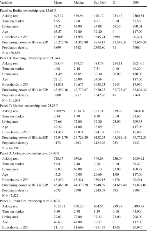
Table 1 Descriptive statistics of selected variables
Variable Mean Median Std. Dev. Q1 Q99
Panel A: Berlin, ownership rate: 15.61%
Asking rent 692.37 549.94 470.12 233.42 2500.35
Time on market 5.95 2.60 8.71 0.10 55.50
Living area 74.27 67.00 34.08 29.50 200.01
Age 65.57 59.00 39.20 0 117.00
Households in ZIP 12,008 11,997 3645.74 3890 20,434
Purchasing power of HHs in ZIP 35,272.76 34,352.80 4954.13 27,548.31 52,669.38
Population density 3899 3542 2398.80 61 7908
N = 180,858
Panel B: Hamburg, ownership rate: 21.14%
Asking rent 795.44 658.55 483.79 254.11 2624.01
Time on market 4.98 2.10 7.51 0.10 40.20
Living area 71.49 65.65 30.30 26.00 180.00
Age 52.12 52.00 34.56 0 117.00
Households in ZIP 11,051 10,677 3458.73 2143 17,979
Purchasing power of HHs in ZIP 43,559.36 42,779.87 7670.23 32,723.47 63,894.32
Population density 3800 3757 2342.76 45 7560
N = 101,008
Panel C: Munich, ownership rate: 25.23%
Asking rent 1209.59 1034.08 721.71 379.96 3960.00
Time on market 3.84 1.70 6.30 0.10 33.60
Living area 77.66 72.00 37.20 23.00 209.33
Age 42.22 41.00 33.69 0 117.00
Households in ZIP 11,459 12,074 3241.20 3573 16,896
Purchasing power of HHs in ZIP 55,942.79 54,728.80 6132.63 45,586.18 69,752.31
Population density 4173 4463 2184.26 253 7933
N = 47,394
Panel D: Cologne, ownership rate: 27.42%
Asking rent 720.55 639.6 369.88 250.00 2039.92
Time on market 5.04 2.40 7.28 0.10 39.47
Living area 72.03 68.00 30.13 23.00 168.97
Age 45.24 46.00 29.60 1.00 117.00
Households in ZIP 13,452 13,521 3594.13 6176 20,561
Purchasing power of HHs in ZIP 45,466.38 44,370.20 5748.89 34,685.48 58,827.02
Population density 3675 3390 2243.07 395 7598
N = 47,527
Panel E: Frankfurt, ownership rate: 20.67%
Asking rent 1012.81 850.20 634.55 299.98 3499.85
Time on market 5.89 2.70 8.29 0.10 45.90
Living area 79.03 72.00 37.23 23.00 208.00
Age 49.63 47.00 39.57 0 117.00
Households in ZIP 11,147 11,669 4351.39 1546 20,945
This table reports selected descriptive statistics, the ownership rate and the number of observations for each of the seven cities. The ownership rates are as of 2013. The data consists of 482,196 observations on the residential rental market. The sample period is 2013 Q1 to 2017 Q4
Table 1 (continued)
Variable Mean Median Std. Dev. Q1 Q99
Purchasing power of HHs in ZIP 47,528.31 46,692.74 6663.02 37,419.27 76,088.03
Population density 3930 4194 2098.80 146 7785
N = 41,446
Panel F: Stuttgart, ownership rate: 32.92%
Asking rent 910.71 775.20 501.26 270.98 2749.82
Time on market 3.73 1.60 5.93 0.10 30.40
Living area 79.19 74.00 34.29 23.00 193.01
Age 50.25 48.00 34.85 0 117.00
Households in ZIP 10,385 10,927 3098.97 1104 15,899
Purchasing power of HHs in ZIP 47,058.05 46,374.77 4440.57 40,041.62 61,972.64
Population density 3507 3353 1766.72 254 7404
N = 17,967
Panel G: Dusseldorf, ownership rate: 24.08%
Asking rent 762.86 630.00 486.69 240.00 2579.00
Time on market 6.60 3.20 8.91 0.10 50.01
Living area 75.65 70.00 33.85 25.00 190.00
Age 52.18 54.00 29.78 1.00 117.00
Households in ZIP 9726 9703 3021.54 2721 15,045
Purchasing power of HHs in ZIP 47,869.27 46,140.99 5851.67 40,382.03 65,472.45
Population density 3999 3913 2370.53 23 7906
N = 45,996
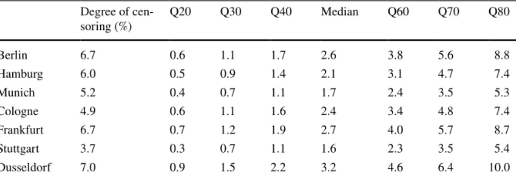
Table 2 Degree of censoring and average time on market in weeks per quantile
This table reports the degree of censoring and the average time on market in weeks for the seven cities.
The data consists of 482,196 observations on the residential rental market. The sample period is 2013 Q1 to 2017 Q4
Degree of cen-
soring (%) Q20 Q30 Q40 Median Q60 Q70 Q80
Berlin 6.7 0.6 1.1 1.7 2.6 3.8 5.6 8.8
Hamburg 6.0 0.5 0.9 1.4 2.1 3.1 4.7 7.4
Munich 5.2 0.4 0.7 1.1 1.7 2.4 3.5 5.3
Cologne 4.9 0.6 1.1 1.6 2.4 3.4 4.8 7.4
Frankfurt 6.7 0.7 1.2 1.9 2.7 4.0 5.7 8.7
Stuttgart 3.7 0.3 0.7 1.1 1.6 2.3 3.5 5.4
Dusseldorf 7.0 0.9 1.5 2.2 3.2 4.6 6.4 10.0
on market quantiles from the 0.2 to the 0.8 quantile. The top and bottom end of the time on market distribution display extremely high and extremely low values respectively and hence are not the subject of this analysis.
Table 1 shows the descriptive statistics for the variables of interest for each of the seven cities. Comparing the seven cities shows that the mean time on market is fairly low in Stuttgart and Munich and relatively high in Dusseldorf, Berlin and Frank- furt. With 3.73 weeks, the mean time on market is lowest in Stuttgart and highest in Dusseldorf with 6.6 weeks. Table 2 shows the time on market for each of the selected quantiles and for all seven cities. It confirms that the time on market is low- est in Stuttgart and Munich and highest in Dusseldorf, Frankfurt and Berlin along the entire distribution. Furthermore, Table 2 exhibits the degree of censoring present in the data for each city. The degree of censoring can be interpreted as the percent- age of dwellings that have not been taken out of the MLS until the cut of date. For example, in Berlin 6.7% of all dwellings that appeared in the MLS from 2013 Q1 to 2017 Q4 still remain in the MLS after the last day of the observation period.
The covariate of asking rent is lowest in Berlin with a mean of 692.37 € and highest in Munich with a mean of 1209.59 €. Interestingly, these cities respectively exhibit the lowest and highest mean purchasing power of 35,272.76 € in Berlin and 55,942.79 € in Munich. Furthermore, they are characterized having on average the oldest and youngest buildings respectively. This indicates high development activ- ity in the more recent past in Munich. These variables reveal interesting differences between the cities and give rise to an individual investigation of each city.
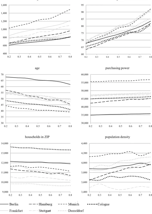
The aim of the study is to investigate the impact of changes in the explanatory variables on the time on market of rental dwellings, divided by their liquidity level.
Hence, it is of special interest whether there are patterns in the dwelling charac- teristics, which might explain the affiliation to a respective liquidity quantile. Fig- ure 2 shows that across all seven cities, the dwellings in the most liquid quantile, 0.2 (Q20), are on average the cheapest, the smallest and the oldest. Furthermore, they are located in ZIP code areas with the lowest purchasing power, but a rela- tively large number of households. In contrast to the most liquid quantile, dwell- ings assigned to the 0.8-quantile (Q80) display on average 33.71% higher rents, are 25.3% larger, 12.13% younger, located in ZIP codes with 2.67% higher purchasing power, have 3.46% less households in a ZIP code area and are 3.05% more densely populated. These insights based on pure analysis of descriptive statistics give rise to the assumption that the level of time on market strongly depends on the character- istics of a dwelling. Hence, this supports the CQR approach to get a deeper under- standing of the determinants of time on market.
5 Results
5.1 Results of the cox survival regression
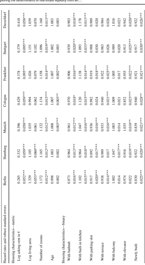
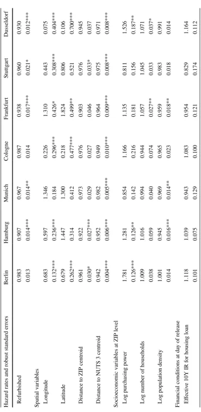
In a first step, covariates raising or lowering the time on market of rental dwellings of the seven largest German cities have been considered. The results of the Cox sur- vival regressions are presented in Table 3. Since the results are displayed as hazard
400 600 800 1,000 1,200 1,400 1,600
0.2 0.3 0.4 0.5 0.6 0.7 0.8
asking rent
60 65 70 75 80 85 90 95
0.2 0.3 0.4 0.5 0.6 0.7 0.8
living area
30 35 40 45 50 55 60 65 70
0.2 0.3 0.4 0.5 0.6 0.7 0.8
age
30,000 35,000 40,000 45,000 50,000 55,000 60,000
0.2 0.3 0.4 0.5 0.6 0.7 0.8
purchasing power
9,000 10,000 11,000 12,000 13,000 14,000
0.2 0.3 0.4 0.5 0.6 0.7 0.8
households in ZIP
3,400 3,600 3,800 4,000 4,200 4,400
0.2 0.3 0.4 0.5 0.6 0.7 0.8
population density
Fig. 2 Descriptive development of selected covariates for time on market quantiles. This figure displays descriptive statistics for selected variables across seven time on market quantiles for the seven largest German cities. The time on market quantiles are labelled on the x-axis and the respective diagram title is labelled on the y-axis. Altogether, the data consists of 482,196 observations on the residential rental mar- ket. The sample period is 2013 Q1 to 2017 Q4
Table 3 Results of the Cox survival regression Hazard rates and robust standard errorsBerlinHamburgMunichCologneFrankfurtStuttgartDusseldorf Housing characteristics—metric Log asking rent in €0.2850.3320.3960.4290.3780.3790.410 0.052***0.059***0.058***0.059***0.095***0.095***0.058*** Log living area1.3291.1851.0350.9941.0261.1511.039 0.053***0.060***0.0610.0620.0790.1020.070 Number of rooms1.1721.1651.1221.1341.1581.0961.160 0.012***0.012***0.012***0.015***0.014***0.019***0.013*** Age0.9981.0031.0081.0071.0071.0021.003 0.0020.0020.003***0.003**0.002***0.0030.003 Housing characteristics—binary With bathtub0.8730.9640.9610.9700.9060.9390.903 0.016***0.013***0.012***0.018*0.016***0.020***0.018*** With built-in kitchen1.1020.9641.0471.1201.1381.0931.178 0.015***0.018**0.016***0.015***0.014***0.033***0.013*** With parking slot0.9170.8920.9360.9820.9190.9880.989 0.020***0.017***0.016***0.0240.018***0.0300.020 With terrace0.9380.9890.9330.9400.9220.9830.984 0.014***0.0170.016***0.021***0.025***0.0260.026 With balcony1.0021.0471.0031.0091.0050.9891.016 0.0140.017***0.0140.0210.0170.0200.023 With elevator0.9740.9161.0350.8520.9550.9130.942 0.0220.019***0.018**0.023***0.022***0.025***0.020*** Newly built0.8300.9220.8390.9400.9210.9170.922 0.025***0.020***0.021***0.028**0.021***0.030***0.026***
Table 3 (continued) Hazard rates and robust standard errorsBerlinHamburgMunichCologneFrankfurtStuttgartDusseldorf Refurbished0.9830.9070.9670.9870.9380.9600.930 0.0130.014***0.014**0.0140.017***0.021*0.012*** Spatial variables Longitude0.6830.5971.3460.2261.3100.4430.075 0.132***0.236***0.1840.296***0.426*0.308***0.404*** Latitude0.6791.4471.3000.2181.8240.8060.106 0.262***0.3140.4120.477***0.499**0.5210.700*** Distance to ZIP centroid0.9610.9220.9730.9760.9030.9760.945 0.030*0.027***0.0290.0270.0460.033*0.037 Distance to NUTS 3 centroid0.9420.9520.9820.9490.9640.9750.971 0.004***0.006***0.005***0.010***0.009***0.008***0.008*** Socioeconomic variables at ZIP level Log purchasing power1.7811.2810.8541.1661.1350.8111.526 0.126***0.126**0.1420.2160.1810.1560.187** Log number of households1.0091.0160.9940.9441.0571.0451.071 0.0380.0590.0400.0740.027**0.0330.037* Log population density1.0010.9450.9690.9650.9590.9830.991 0.0140.016***0.014**0.0230.018**0.0180.014 Financial conditions at day of release Effective 10Y IR for housing loan1.1181.0390.9431.0830.9540.8291.164 0.1010.0750.1290.1000.1210.1740.112
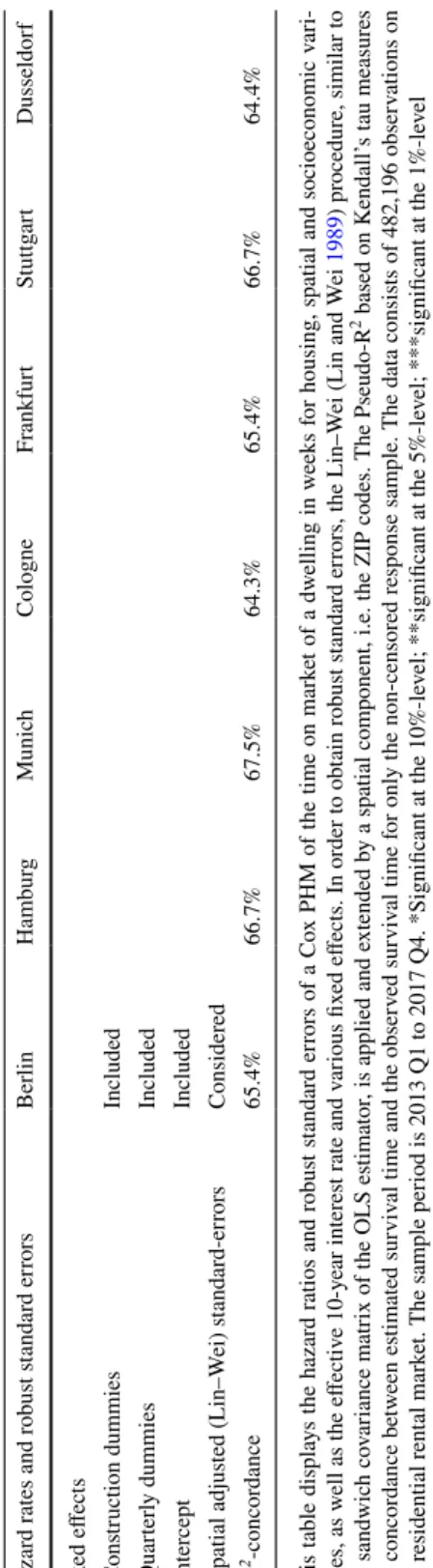
Table 3 (continued) Hazard rates and robust standard errorsBerlinHamburgMunichCologneFrankfurtStuttgartDusseldorf Fixed effects Construction dummiesIncluded Quarterly dummiesIncluded InterceptIncluded Spatial adjusted (Lin–Wei) standard-errorsConsidered R2-concordance65.4%66.7%67.5%64.3%65.4%66.7%64.4% This table displays the hazard ratios and robust standard errors of a Cox PHM of the time on market of a dwelling in weeks for housing, spatial and socioeconomic vari- ables, as well as the effective 10-year interest rate and various fixed effects. In order to obtain robust standard errors, the Lin–Wei (Lin and Wei 1989) procedure, similar to the sandwich covariance matrix of the OLS estimator, is applied and extended by a spatial component, i.e. the ZIP codes. The Pseudo-R2 based on Kendall’s tau measures the concordance between estimated survival time and the observed survival time for only the non-censored response sample. The data consists of 482,196 observations on the residential rental market. The sample period is 2013 Q1 to 2017 Q4. *Significant at the 10%-level; **significant at the 5%-level; ***significant at the 1%-level
rates, a rate larger than one decreases the time on market and thus increases liquid- ity, while a rate smaller than 1 decreases liquidity. The results show that an increase in the asking rent ceteris paribus, leads to a longer time on market across all seven cities. The same direction of the effect was found by Cajias and Freudenreich (2018).
The seller faces the trade-off between the time the dwelling is on the market and the price he might receive, as mentioned by Anglin et al. (2003) for the real estate trans- action market. According to that, the result is not surprising, that a higher asking rent leads to lower liquidity of dwellings. Since the densely populated cities regu- larly display an excess demand for housing, it is of particular interest to investigate the rental effect for individual liquidity quantiles, as the magnitude of these effects is supposed to differ widely along the distribution. Miller (1978) postulates that hous- ing attributes, defining its attractiveness, are important determinants of time on mar- ket. An increase in living area significantly increases liquidity in two of seven cities, namely Berlin and Hamburg. As Hamburg is the city with the smallest average liv- ing area in this sample, people might desire larger apartments and hence take them off the market faster. Cologne is the only city where living area has a prolonging impact on time on market, however, is not significant. A segmentation into liquidity quantiles might be useful in order to consider the impact and its significance of, for instance, the living area for each quantile, as it might be the heterogeneity within the cities that leads to insignificant effects. The number of rooms in a dwelling, in contrast, has a statistically significant positive effect on liquidity for all seven cities.
Hence, it seems that in most of these seven highly demanded regions, a larger dwell- ing in general is not favorable. A dwelling with a larger number of rooms, however, can provide more living space for more people and thus is highly demanded and consequently off the market more quickly. Surprisingly, the marketing time is ceteris paribus shorter, the older the dwelling, and is longer for newly built and refurbished ones. In Berlin the marketing time is longer the older the building, however, the effect is not statistically significant. This might be due to the fact, that in this sample Berlin exhibits by far the highest average building age. An increase in the distance to the NUTS 3 centroid, which is used as a proxy for the city center, is associated with a longer time on market. This seems obvious, as regions farer away from the city center are less demanded. The distance to the ZIP code centroid shows almost no statistically significant impact. The coefficients of each socioeconomic factor are not significant for most cities, again emphasizing the importance of considering each time on market quantile separately. A higher purchasing power results on average in a shorter time on market in Berlin, Hamburg, and Dusseldorf, all else equal, whereas for the remaining cities, the effect is not statistically significant. Among the seven cities, Berlin and Hamburg are the cities with the lowest average purchasing power, hence this result points to the fact that in Berlin and Hamburg people would spend additional purchasing power on the search and matching process that would shorten marketing time. While an increase in the number of households significantly reduces time on market in Frankfurt and Dusseldorf, the population density has a significant prolonging effect on time on market in Hamburg, Munich, and Frankfurt. It should be noted that neither socioeconomic variable has an impact on time on market in Cologne and Stuttgart. The Pseudo-R2 based on Kendall’s tau, which measures the concordance between estimated survival time and the observed survival time for the
non-censored response sample, ranges from 64.3 to 67.5%. Those values are com- mon in survival studies. At this point it is necessary to note that these values cannot be interpreted directly or compared to the usual R2 calculated for OLS regressions.
5.2 Results of the censored quantile regression
In a second step, the same regressors as for the Cox survival regressions are used to estimate CQRs, in order to gain deeper insight into the time on market quantiles.
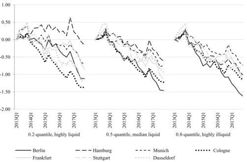
Therefore, for each city, the sample of dwellings was divided into time on market quantiles from the 0.2- to the 0.8-quantile. The results for the covariates of interest are shown in Figs. 3, 4, 5 and 6. In Figs. 4, 5 and 6 the black lines plot the esti- mated coefficients, the grey lines display the standard deviations. Each plot shows the development of a coefficient 𝛽k𝜏 . over the liquidity quantiles 𝜏 . for each of the seven cities k. A positive statistically significant coefficient increases time on mar- ket, thus decreasing liquidity, while a negative statistically significant coefficient has the opposite effect. The main effects, divided into quarterly factors, housing charac- teristics, spatial gravity variables, and socioeconomic characteristics, are reported below. The crucial point is that, contrary to the traditional regression models, the effect of a change in the covariate holds for the same quantile 𝜏 , rather than across quantiles.5
-2.00 -1.50 -1.00 -0.50 0.00 0.50 1.00
2013Q1 2014Q1 2015Q1 2016Q1 2017Q1 2013Q1 2014Q1 2015Q1 2016Q1 2017Q1 2013Q1 2014Q1 2015Q1 2016Q1 2017Q1
0.2-quantile, highly liquid 0.5-quantile, median liquid 0.8-quantile, highly illiquid
Berlin Hamburg Munich Cologne
Frankfurt Stuttgart Dusseldorf
Fig. 3 Estimated quantile regression coefficients of the quarterly dummy variables. The figure displays the development of the coefficients 𝛽k𝜏 of the quarterly dummy covariate for the 0.2-, 0.5- and 0.8-quan- tile for each of the seven cities k over time. Altogether, the data consists of 482,196 observations on the residential rental market. The sample period is 2013 Q1 to 2017 Q4
5 Table A2 in the Online Appendix shows the estimated coefficients for all cities and quantiles.
5.3 Quarterly time effects
The considered period is characterized by low interest rates, high migration to Ger- many, specially to the metropolises, and additionally far too low housing supply in these cities. Consequently, vacancy has mostly been diminishing, and real estate prices as well as rents increasing. Despite rising construction activity in most cit- ies, building completion was insufficient to meet demand, leading to excess demand.
Time fixed effects as quarterly dummies have been included in the estimation equa- tion to capture these developments over time and its impact on the time on market.6 This time trend can be observed in Fig. 3 for each city and for quantiles represent- ing high, medium and low liquidity. The base quarter is the first quarter of 2013, so that all changes are with respect to this basis. All in all, time on market has been decreasing compared to the base quarter for all time on market quantiles and for each city. However, the magnitude and direction of change differs between the cit- ies and different time on market quantiles. In the first quarter of the year, time on the market is usually relatively low for rental dwellings. Hence, in 2013 and partly in the beginning of 2014 time on market has been increasing relative to the base quarter in all cities and all time on market quantiles. Over the course of 2014 time on market started to decrease relative to 2013 Q1 in six of the seven cities and all time on market quantiles. The exception is Hamburg, where time on market started to decrease relative to 2013 Q1 later than in all other cities and it is striking that the date of decline is documented later for more liquid quantiles. This supports the importance of analyzing all cities separately. Furthermore, it emphasizes the hypoth- esis that the time on market development within a city might be different for distinct time on market quantiles and thus the quantiles should be analyzed separately. By far the most pronounced decline in time on market experienced Berlin in the 0.5 and 0.8 quantile. In the 0.2 quantile the development in Berlin is rather average com- pared to the other cities as a sharp decline only starts in 2017. Hence, it seems that in Berlin relative to 2013 Q1 the demand for rental dwellings was higher in the 0.5 and 0.8 quantile. As described in Sect. 4. Data and Descriptive Statistics, the living area of dwellings in these quantiles is relatively larger than in the 0.2 quantile. A reason for this result might be the development of household members during the recent years. According to Vonovia and CBRE (2016), in 2014, the year when time on market started to decline compared to the base quarter, Berlin was amongst the cities with the highest percentage of single households and even had the highest per- centage of one- and two-person-households together. Hence, the demand for larger dwellings was probably relatively small compared to the other cities. According to
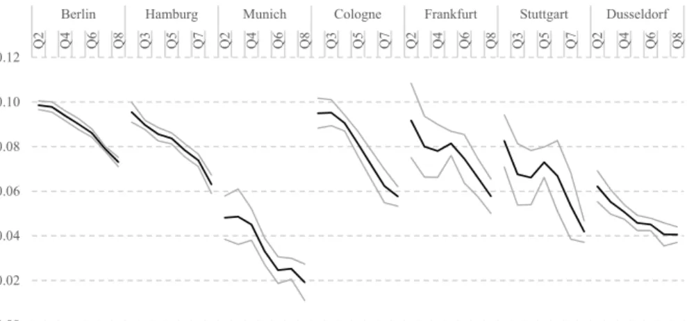
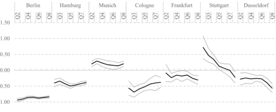
Fig. 4 Estimated quantile regression coefficients of selected housing variables. The figure displays the development of the coefficients 𝛽k𝜏 of the housing covariates across the liquidity quantiles τ for each of the seven cities and the respective confidence intervals. The impact of an individual coefficient is insig- nificant if the confidence interval includes zero. The data consists of 482,196 observations on the resi- dential rental market. The sample period is 2013 Q1 to 2017 Q4
▸
6 Of those quarterly effects, 82.0% are significant at the 10% significance level, while 74.5% are signifi- cant at the 5% significance level.
Log asking rent
Age
With balcony
1.00 1.20 1.40 1.60 1.80 2.00 2.20 2.40 2.60
2.80 Q2 Q4 Q6 Q8 Q3 Q5 Q7 Q2 Q4 Q6 Q8 Q3 Q5 Q7 Q2 Q4 Q6 Q8 Q3 Q5 Q7 Q2 Q4 Q6 Q8 Berlin Hamburg Munich Cologne Frankfurt Stuttgart Dusseldorf
-0.03 -0.02 -0.02 -0.01 -0.01 0.00 0.01 0.01 0.02 0.02
-0.15 -0.10 -0.05 0.00 0.05 0.10 0.15
Q2 Q4 Q6 Q8 Q3 Q5 Q7 Q2 Q4 Q6 Q8 Q3 Q5 Q7 Q2 Q4 Q6 Q8 Q3 Q5 Q7 Q2 Q4 Q6 Q8 Berlin Hamburg Munich Cologne Frankfurt Stuttgart Dusseldorf