Erlangung der Doktorwürde der
Naturwissenschaftlich-Mathematischen Gesamtfakultät
der
Ruprecht-Karls-Universität Heidelberg
vorgelegt von
Dipl.-Phys. Dirk Engelmann
aus Tübingen
Tag der mündlichen Prüfung: 26. Juli 2000
Gutachter: Prof. Dr. Bernd Jähne
Prof. Dr. Kurt Roth
of the Rupertus Carola University of Heidelberg, Germany
for the degree of Doctor of Natural Sciences
3D-Flow Measurement by Stereo Imaging
presented by
Diplom-Physicist: Dirk Engelmann
born in: Tübingen, Germany
Heidelberg, July 26, 2000
Referees: Prof. Dr. Bernd Jähne Prof. Dr. Kurt Roth
A new method to record three-dimensional liquid flow fields by using ‘Particle Tracking Velocimetry’ is presented. It is based on a two-dimensional Particle Tracking Velocimetry method. It was extended to the third space dimension in order to include the complete physical space. This procedure allows to determine the Lagrange-flow field and to calculate from it the Euler-velocity flow field ob- tained from many other flow measuring techniques.
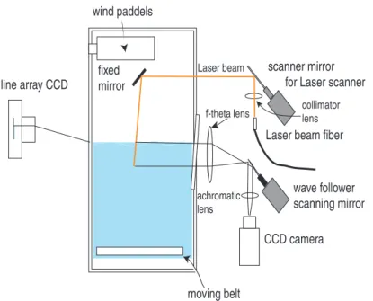
A calibration method was developed for the wind-wave-flume which allows a high resolution in space. The stereo camera setup and the experimental setup were optimized for the liquid flow measurements. For the first time a liquid prism and a Scheimpflug-camera geometry was used.
Numerical calculations using the finite element method demonstrate the complex- ity of the problem of dealing with free surfaces with wind-induced shear forces as a boundary condition. They show clearly that experimental studies are indispensable for describing phenomena such as ‘bursts’ (descending of liquid elements from close to the surface into deeper layers).
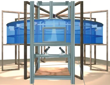
Flow measurements were performed in a newly constructed wind-wave-flume (AEOLOTRON) and in a smaller predecessor by using the newly developed ima- ging methods. In this way the flow fields of wind driven water waves could be characterized by the velocity field and the ‘turbulence’ conditions.
Zusammenfassung
Ein neues Verfahren zur Messung des dreidimensionalen Strömungsfeldes mittels
‘Particle Tracking Velocimetry’ wird vorgestellt. Ein zweidimensionales Parti- cle Tracking Velocimetry liegt dem Verfahren zugrunde. Es wurde auf die dritte Raumdimension erweitert, um den gesamten physikalischen Raum zu erfassen.
Dieses Verfahren erlaubt, das Lagrange´sche Strömungsfeld zu bestimmen, woraus auch das von vielen anderen Verfahren erhaltene Euler´sche Geschwindigkeitsfeld berechnet werden kann.
Das für den Einsatz am Wind-Wellen-Kanal entwickelte Kalibrierverfahren er- möglicht eine hohe räumliche Auflösung. Der Stereokamera-Aufbau und der Ver- suchsaufbau wurde für die Strömungsmessungen optimiert. Dabei wurde erstmals ein Flüssigkeitsprisma und eine Scheimpflug-Kamera-Anordnung eingesetzt.
Numerische Rechnungen unter Verwendung der finite Elemente-Methode zeigen die Komplexität des Problems, freie Wasseroberflächen mit windinduzierten Scher- kräften als Randbedingung zu behandeln. Sie machen deutlich, daß experimentelle Untersuchungen unerlässlich sind, um Phänomene wie ‘bursts’ (Abtauchen von oberflächennahen Flüssigkeitselementen in tiefere Schichten) zu beschreiben.
(AEOLOTRON) und am kleineren Vorgängermodell mit dem neuentwickelten Bild- verarbeitungsverfahren durchgeführt. Die Strömungsfelder von windinduzierten Wasserwellen konnten auf diese Weise Geschwindigkeitsfeld und “Turbulenzzu- stand” charakterisiert werden.
1 Introduction 1 2 Theoretical aspects of liquid flow and gas exchange 3
2.1 Description of a liquid flow field . . . 3
2.2 Gas transfer processes . . . 4
2.3 Numerical solutions and models . . . 11
3 Flow visualization 19 3.1 Flow-field measurement techniques . . . 19
3.1.1 Hot wire anemometry . . . 20
3.1.2 Laser Doppler anemometry (LDA), acoustic Doppler ve- locimetry (ADV) . . . 20
3.1.3 Particle imaging velocimetry (PIV) . . . 21
3.1.4 Particle tracking velocimetry (PTV) . . . 21
3.2 Techniques for flow field visualization . . . 22
3.2.1 Seeding particles . . . 22
3.2.1.1 Scattering properties . . . 23
3.2.1.2 Buoyancy . . . 28
3.2.2 Hydrogen/oxygen bubbles . . . 30
3.3 Experimental setup for particle tracking velocimetry . . . 31
3.3.1 Traditional setup . . . 31
3.3.1.1 Observation close to the water surface . . . 31
3.3.2 Stereo setup . . . 33
3.3.2.1 Heidelberg circular wind-wave facility . . . 33
OLOTRON) . . . 35
3.3.2.3 Volume of observation for stereo camera setup . 37 3.3.2.4 Technical data of used imaging devices . . . 38
3.3.3 Improvements for stereoscopic flow visualization . . . 40
3.3.3.1 Scheimpflug stereo camera setup . . . 41
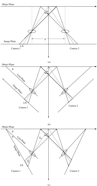
4 Geometry of the stereoscopic system 45 4.1 Model of the stereoscopic system . . . 45
4.2 A simple camera model . . . 47
4.2.1 Homogeneous coordinate system . . . 47
4.2.2 Pinhole camera model . . . 48
4.2.3 Pinhole camera model including intrinsic camera parameters 49 4.2.4 The linear camera model . . . 50
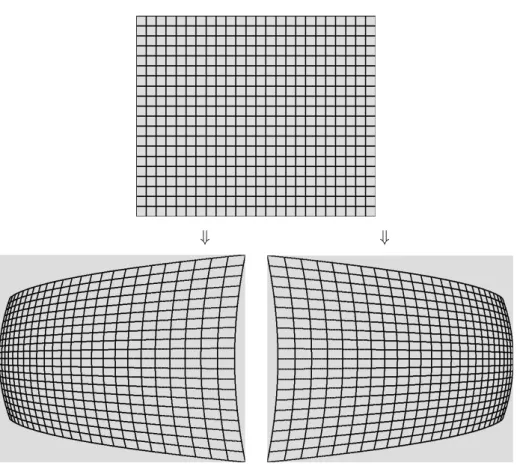
4.2.5 Camera model including lens distortion . . . 52
4.2.6 Camera model and the Scheimpflug condition . . . 54
4.3 Multiple media geometry . . . 56
5 Image sequence analysis for stereo PTV 59 5.1 Calibration . . . 59
5.1.1 The choice of the calibration target . . . 60
5.1.2 The calibration procedure . . . 61
5.2 The particle tracking velocimetry (PTV) algorithm . . . 64
5.2.1 Segmentation . . . 65
5.2.1.1 Region oriented segmentation . . . 66
5.2.1.2 Model-based method . . . 69
5.2.2 Labeling and position determination of a particle . . . 70
5.2.3 Correspondence solving . . . 71
5.2.3.1 Particle characteristics . . . 72
5.2.3.2 Velocity estimation . . . 75
5.2.3.3 PTV post processing . . . 75
5.3 Stereo correspondence solving . . . 76
5.3.3 Applied constraints for 3D PTV . . . 83 5.3.4 Stereo correlation algorithm . . . 84
5.3.4.1 Application of the geometric and ordering con- straint . . . 84 5.3.4.2 Object property constraint . . . 86 5.3.5 Stereo coordinate reconstruction . . . 87
6 Analysis of data and discussion of results 93
6.1 Calibration and resolution . . . 93 6.2 Stereo correspondence . . . 95 6.3 Stereo particle tracking velocimetry . . . 98
7 Outlook 115
A Data tables 117
B Linearized wave equation 121
C Depth of field, depth of focus 123
D Basics of the finite element method 125
Introduction
The major part of the earth is covered by oceans. Gas from the atmosphere is transported into the oceans due to exchange processes at the surface. For gases such as CH4, O2or CO2the oceans are a major sink. About 90% of the global CO2
is dissolved in the oceans. But the amount of CO2- one of the most important gases concerning the prediction of climatic changes - transfered from the atmosphere to the oceans is still uncertain and under debate. Estimations deviate by±2 Gt from 4 Gt. The concentrations of these gases in the atmosphere influence the climate significantly. It is therefore important to understand air-sea related gas exchange processes.
The atmospheric gas has to pass the air-water phase boundary and the amount of gas transported per time is characterized by the transfer velocity. The transfer through the air-water boundary is controlled by a microscopic layer (20-300 µm, Münsterer [1996]) at the water surface in which molecular diffusion is the domi- nating transport process. Beneath this layer turbulent transport is the far more efficient transport mechanism. Water waves affect the gas transport and they show a large variety of different types. On a scale of some centimeters up to several kilometers gravitational waves appear where gravitation is the restoring force. On a smaller scale of millimeters up to centimeters capillary waves show up. Here the surface tension is the restoring force. If air flows over the free surface of the liquid and capillary waves are generated, the transfer of gas in the liquid is considerably increased. The appearance of wind driven water waves is clearly associated with an increase in the gas transfer rate. This effect is well known, but the underlying physical mechanisms are not fully understood. The parameterization of the sur- face shape is an attempt to characterize the gas transport. The mean square slope was found by Jähne [1985] to be an important parameter. Furthermore the liquid flow field is of importance in order to understand the physical mechanisms in more detail. Air-water gas transport is also important in the field of chemical engineer- ing. For instance gas-liquid reactors are frequently used where the transport of gas drives chemical reactions.
The aim of this work was to study the liquid flow field close to the free air-water surface. A stereo particle tracking velocimetry algorithm was applied and im- proved. It allows to study the liquid flow field in three-dimensional space. This technique is a major improvement to the well established two-dimensional parti- cle tracking velocimetry by which a two-dimensional flow field is obtained. Since the liquid flow is a three-dimensional phenomenon it is important to study the complete flow field by a stereoscopic method. The particle tracking velocimetry method allows to study the Lagrange-velocity flow field and is therefore especially well suited to study the transport of near surface water elements to the deeper water.
New techniques for the visualization of the liquid flow where introduced.
The theoretical background of liquid flow field, gas exchange processes and nu- merical methods are given in chapter 2. In chapter 3 frequently applied flow visu- alization methods are introduced and the associated techniques for the flow field evaluation are explained. The stereoscopic geometry and the modeling of the used system are shown in chapter 4. The image sequence processing techniques are explained in chapter 5 and the results are presented and discussed in chapter 6. Fi- nally future steps and tasks for image sequence processing and for improving the experimental setup are proposed in the ‘outlook’ chapter 7.
Theoretical aspects of liquid flow and gas exchange
2.1 Description of a liquid flow field
The motion of fluids can be described in one of two ways. The way of description implies directly the experimental techniques to be used (section 3.2).
The first way, the Euler-description of motion, regards the physical quantities such as the velocity−→u , pressure p and densityρas functions of position−→x and time t.
Thus −→u =−→u(−→x,t) (2.1)
(same for p andρ) represents the velocity at prescribed points in space-time. The derivatives with respect to−→x and t represent the gradient field at a given time and a given position.
Alternatively, the fluid motion can be described in the Lagrange way. Fluid ele- ments are identified at some initial time towith position−→xo. Thus−→x =−→x(−→xo,t− to)where −→x(−→xo,0) =−→xo. The velocity of a fluid element is therefore the time derivative of its position:
−
→u(−→xo,t−to) = ∂
∂t−→x(−→xo,t−to) (2.2) The total time derivative is written in Euler-terms as
d dt = ∂
∂t+ (−→u ·∇) (2.3)
which is the sum of the rate of change at a fixed point and a convective rate of change.
Many instruments measure fluid properties at a fixed point and provide Euler-flow field information directly. Questions concerning diffusion and mass transport deal with the motion of fluid elements and thus the Lagrange specification of the prob- lem is better suited to treat them. The Lagrange description implies a marking of fluid elements by a dye or other tracers.
The equations of motion are governed by the conservation laws of mass and mo- mentum:
The momentum transport is expressed by the Navier-Stokes equation:
∂−→u
∂t + (−→u ·∇)−→u −ν∆−→u +∇p=−→f (2.4) where−→f is the resultant of all forces acting on the fluid (such as the gravitational force−→g ) andνthe viscosity of the fluid.
The conservation of mass (continuity equation) is expressed as
∂ρ
∂t +∇·(ρ−→u) =0 (2.5)
and if the density of a fluid element does not change it takes the form
∇· −→u = 0 (2.6)
For an unsteady, diffusive mass transport Fick’s 2ndlaw applies:
∂c
∂t +−→u ·∇c=D∆c (2.7)
where c is the gas concentration and D the diffusion coefficient.
The flux density is related to the concentration gradient and defined as−→j =−D∇c.
The water (in oceanic and laboratory circumstances considered in this work) can be regarded as an isotropic, incompressible Newtonian fluid1.
2.2 Gas transfer processes
As the transport of atmospheric gases (inert and sparingly soluble) is the physical background of this work, a short overview of models describing basic processes is given.
1pi j=−pδi j+2νei j, with strain tensor ei j=12(∂u∂xi
j+∂∂xuj
i)
The transport of inert or sparingly soluble gases between air and water is controlled by molecular transport (diffusion) and by turbulent transport processes. Directly at the water surface molecular diffusion is the process controlling the gas transfer.
Turbulent transport vanishes at the water surface2.
Molecular diffusion is caused by differences in the gas concentration. This is de- scribed by Fick´s 1stand 2nd law.
Fick´s 1stlaw is written as
−
→j =−D∇c (2.8)
and describes the proportionality of the flux density−→j to the concentration gradi- ent of the gas∇c where D is the proportionality constant.
Fick´s 2ndlaw is written as dc dt =∂c
∂t+−→u ·∇c=−∇j=D∆c (2.9) and describes the diffusive transport of mass (generally of scalar tracers). The transport is included in the term−→u ·∇c.
The amount of gas transported through the water surface per time is quantified by the gas transfer velocity
−
→k =
−
→j
∆c (2.10)
and∆c=csur f ace−cbulkis the gas concentration difference between the water sur- face and the water bulk3.
The velocity−→u is determined by the Navier-Stokes equation
∂−→u
∂t + (−→u ·∇)−→u =ν∆−→u +1 ρ−→f −1
ρ∇p (2.11)
where−→f is the sum of outer forces,∇p the pressure gradient andρthe fluid density.
−
→u ·∇u is the convective term andν∆u the viscous term whereνis the kinematic viscosity.
In order to understand the physical properties of the flow better, frequently a pertur- bation approach (see Monin and Yaglom [1975]) is used to deal with the equations (2.9) and (2.11). The perturbation is in−→u and c, expressed by−→u =−→u +−→u0 and c=c+c0(barred characters mean average over time, primed characters the fluctu- ating part).
2The derivative of a ‘mass element’ at the water surface z=0 in time is∂η∂t|z=0 =0.
3‘water bulk’: below a reference depth the mixing of concentration is large and no concentration gradient is present.
Substituting this into equation (2.9) and taking the temporal average<·>yields
∂c
∂t +−→u∇c=−∇(<c0−→u0>−D∇c)
| {z }
−
→j
(2.12)
(where the identity−→u ·∇c=∇·(−→u c)−c·∇·−→u was applied).−→j is the flux density which is the sum of the average molecular diffusion and the turbulent fluxes.
Applying the same substitution to equation (2.11) and considering the case of−→u in x-direction and depending only on z yields
∂u
∂t =−∇(<u0w0>−ν∇u)
| {z }
=: jm/ρ
(2.13)
where−→u =
u+u0
v0 w0
.
The first term is called Reynolds stress (in three dimensions this term ti j =u0iu0j is a symmetric second-order tensor for u,i,j ={u0,v0,w0}). It describes the turbulent transport and the second term describes the viscous transport. For the stationary case ∂∂tu =0, jm is a flux density of momentum - similar to equation (2.12). At the water surface the momentum flux density is equivalent to the shear forceτ, jm|z=0 =:τ. This leads to the definition of a measure of the surface friction that has the dimension of a velocity, the friction velocity u2∗:=ρτ. If the viscous term is zero, the friction velocity becomes u2∗=<u0w0>which expresses the correlation of turbulent transport with the fluctuating velocity components (here in x- and z- direction). If laminar flow is considered and the turbulent term is zero, the shear stress tensor becomesτ=νρ∇u. This can for example be caused by wind stress on the water surface.
The terms viscous boundary layer and aqueous mass boundary layer are intro- duced to quantify the momentum transport and the molecular transport, respec- tively. For the definition of the aqueous mass boundary layer thickness z∗the equa- tions (2.8) and (2.10) are taken and with j=−D∂c∂z|z=0 at the water surface4z=0 (assuming the concentration is a function of the depth z, c=c(z)) it follows:
z∗= ∆c
−∂c∂z|z=0
=D∆c j = D
k
where∆c is the concentration difference between the surface and the water bulk.
For the viscous boundary layer it follow fromτ=νρ∂∂zu|z=0 4At the water surface the turbulent transport is absent.
z*
c, u
z z=0
water air
c ws cas
c
u
reference concentration/ momentum (bulk) z
* viscous
molecular
Figure 2.1: Schematic graph of the molecular and the viscous boundary layers on both sides of a gas-liquid interface. Due to the larger solubilityαof the tracer gas in water as compared to air, the tracer gas concentration is discontinuous at the interface (cws=α·cas).
viscous z∗= ∆u ρ∂u∂z|z=0
= ∆u τ/ν=ν
k
where∆u is the velocity difference between the water surface and the velocity in a reference depth.
The boundary layers are shown schematically in figure 2.1. The boundary layer of molecular diffusion (for dissolved inert gases in water) is in the order of 100 to 300 µm. The range of the viscous boundary layer is larger by a factor of 100 to 2000. The Schmidt number Sc represents this relation of the boundary layer thicknesses:
Sc= ν D
The turbulent transport terms of equations (2.12) and (2.13) can be replaced by functions which depend on the depth z and the turbulent diffusion coefficients Kc(z)∂c∂z and Km(z)∂u∂z. The equations can be integrated to obtain the concentration and velocity profiles:
c(z)−c(0) =
z
Z
0
j
D+Kc(z0)dz0, u(z)−u(0) =
z
Z
0
jm/ρ ν+Km(z0)dz0.
Depending on the choice of the coefficients Kc(z)and Km(z)different models are obtained such as the small eddy model and the surface renewal model. They are discussed in the next sections. The models have to deal with the turbulent transport mechanism and the gas diffusion. The simplest model (film model) assumes a stagnant film as a surface layer of thickness z∗where molecular diffusion appears and turbulent transport sets in below this layer. The diffusion of gas through this layer implies a proportionality of the diffusivity D and the gas transfer velocity k=D/z∗.The assumption of a linear concentration profile in the film layer is not very realistic and experimental observations contradicted k∼D (a k∼Dn with n<1 was observed).
Small eddy model
This model describes the turbulent flux through the boundary layer as a cascade of growing eddies. The turbulent diffusion coefficient Kc(z) =D− ∂cj
∂z is determined by a Taylor series expansion applied to the concentration c(z)where the concentra- tion and velocity fluctuations c0,w0 are assumed to be small compared to its mean components. According to Coantic [1986] boundary conditions for a rigid and a free interface5 are applied and the concentration profile c(z)is derived. It shows a lower concentration and a larger decrease in the case of a mobile interface as compared to the rigid interface.
For the gas transfer velocity k the Schmidt number dependency is found as k∼Scnu∗
(for Sc>100) with exponent n=2/3 for the rigid wall and n=1/2 for the free interface.
Surface renewal model
The turbulent transport is based on a statistical renewal rate of the surface layer λ= γzp depending on the depth z. For the classical surface renewal model (Danckwerts [1951]) the exponent p is zero, and for p>0 the renewal rate be- comes zero at the water surface and is more realistic (Jähne [1985]). The gas is transported through the aqueous boundary layer by diffusion and parts of this surface are exchanged with the water bulk in a statistical rateλ. Equation (2.12) becomes
∂c
∂t =D∂2c
∂z2− γzpc
| {z }
=∂z∂<c0w0>
5rigid interface: u0(z=0) =0 and same for v0,w0;∇· −→u0=0→ ∂∂zw0=0, c0(z)|z=0 =0 free interface: w0(z)|z=0 =0, c0(z)|z=0 =0
0.0 0.2 0.4 0.6 0.8 normalized concentration c 8.0
7.0 6.0 5.0 4.0 3.0 2.0 1.0 0.0
normalized depth z
Legende small eddy, n=1/2 small eddy, n=2/3 surface renewal, n=1/2 surface renewal, n=2/3
Figure 2.2: The normalized gas concentration profiles for small eddy and surface renewal model with Schmidt number exponent 1/2 (free boundary, ‘wavy surface’) and 3/2 (rigid boundary, ‘flat surface’).
Applying the boundary conditions6for j yields the mean concentration profile c(z), which is an exponential function for p=0 and an Airy function for p=1. The mean concentration profile shows a larger decrease with depth than the small eddy model which expresses the larger scale turbulence postulated by the surface re- newal rate. The concentration profiles for the surface renewal and the small eddy model are shown in figure 2.2.
The gas transfer velocity k can be predicted (Csanady [1990]) and is found as k∼Scnu∗, where n=1/2 for p=0 and n=2/3 for p=1 interpreted as free and rigid interface respectively.
Influence of wind driven water waves on the gas transfer
If the wind speed over the water surface is increased, surface waves (capillary waves) appear. The gas transfer velocity k changes significantly with the appear- ance of surface waves. This is illustrated in figure 2.3 where k (for CO2) is in- creased with the appearance of waves as compared to a smooth water surface. The transfer velocity k for CO2- which is controlled by the water side - is plotted ver- sus the transfer velocity for water vapor kH2O- which is controlled by the air side.
6All the fluxes through the surface at z=0 and no flux in the bulk z→∞: j(z=0) =D∂c∂z|z=0 =jo
limz→∞j(z) =0
Figure 2.3: Transfer velocity of CO2plotted against the transfer velocity of water vapor (measured in a circular wind-wave facility, Bösinger [1986], Huber [1984], Jähne [1980]). Smooth water surface conditions are marked by circles, wavy con- ditions by stars. The solid line is the prediction of a smooth rigid wall.
The effect of waves on the turbulent transport at the water side is stronger than on the turbulent transport at the air side and results therefore in an asymmetry seen in figure 2.3.
With the occurrence of waves the Schmidt number exponent n decreases (Bösinger [1986]). This indicates the enhanced gas transfer k by a factor of 3, but can not explain the increase of k by up to a factor of 5 from the predictions.
This means, the turbulence level in the mass boundary layer is increased by a fac- tor of 2. Pure surface increase can not explain this effect (Tschiersch and Jähne [1980]).
The wave generation begins at low wind speed (1-5m/s) with capillary waves (wave length in the range of cm). These capillary waves induce turbulent transport close to the water surface, which leads to the increased gas transfer velocity. Therefore this investigation is concerned with effects close to the free water surface in the range of cm. Capillary waves do also appear in connection with gravitational waves which dissipate energy from the gravitational waves (figure 2.4).
The energy flow of wind generated waves is displayed schematically in figure 2.5.
The air flow over the water surface transfers energy and momentum to the wa- ter by the shear stress tensor (which includes pressure, viscous- and Reynolds- stress). The energy is either dissipated in near surface turbulence or to the same amount transfered to water (capillary and gravitational) waves. Due to non linear
Figure 2.4: Gravitational wave and parasitic capillary waves (small ‘ripples’ on the leeward side of the gravitational wave). In the lower image is a view on the water surface where the steepness of the wave is represented by the grey-value, obtained by the imaging slope gauge (ISG, Balschbach [2000]) technique.
wave-wave interaction the capillary and gravitational waves are coupled. Energy of gravitational waves is transfered into capillary waves (parasitic capillary waves) and further transfered to turbulent flow, or directly to turbulent flow by wave break- ing. The breaking of waves is another mechanism for turbulent flow generation.
2.3 Numerical solutions and models
The physical model describes the flow of an incompressible Newtonian fluid7 in an areaΩand time T for a given boundary and initial conditions. The variables sought-after are the velocity−→u(−→x,t) and the pressure p(−→x,t) which are func- tions of time t and the location in physical space−→x = (x1,x2,x3)T. The system is described by the Navier-Stokes (momentum transport) equation and the incom- pressibility condition:
∂−→u
∂t + (−→u ·∇)−→u −ν∆−→u +∇p=−→f
∇· −→u =0 in Ω×T
(2.14)
with outer forces f , the kinematic viscosityν(ρis included in p and f compared to (2.11)).
7Newtonian fluid: The shear stress tensor is defined as Ti j=−pδi j+µ ∂u
∂xij+∂∂uxj
i
; in the one dimensional case the shear stress isτ=µdudy (µ is the coefficient of viscosity, the dynamic viscosity ν=µ/ρ).
waves parasitary capillary
gravitational waves capillary waves
breaking waves micro scale wave
breaking
turbulence
heat surface stress tensor
air flow
wave generation water surface
Figure 2.5: Scheme of interaction processes close to the water surface: The air flow over the water surface transfers momentum and energy via the surface stress into the water. The surface stress generates surface waves which induce gravitational and capillary waves (due to nonlinear interaction). Finally the energy is dissipated to turbulent flow (small scale velocity fluctuations) and into heat.
These equations describe many occurrences in nature such as flow of water or
‘slow’8 air flow, but also serves as a basic model for more complex systems such as combustion processes, chemical reactions, turbulence or multi-phase flow. The mathematical problem to be solved is a time dependent three dimensional nonline- ar partial differential equation (PDE). Because of the nonlinearity of the problem direct solution methods can not be applied and iterative solution methods are re- quired. The type of the problem can vary in time t and spaceΩand this has to be taken into account for the method of solution. If the term(−→u ·∇)−→u −ν∆−→u (equivalent to Re1), the type of PDE has a hyperbolic character, for−ν∆−→u (−→u ·∇)−→u (equivalent to Re'1) the PDE has an elliptic character9. The local character of most of these problems demands also a local refinement in time and space or other techniques which take local properties into account such as multi- grid methods. Without local refinement the capacity of computer memory would by far exceed the availability (a box of a resolution of 100x100x100 points would require 1GByte RAM, if a typical size of 1 KByte storage per point is assumed).
8otherwise the incompressibility condition is not given.
9Second order PDE: Auxx+2Buxy+Cuyy+Dux+Euy+F=0 Let Z=
A B
B C
Elliptical PDE: Z positive definite (det(Z)>0) (i.e. Poisson equation, Laplace equation) Parabolic PDE: det(Z) =0 (i.e. heat conductivity equation, diffusion equation)
Hyperbolic PDE: det(Z)<0 (i.e. wave equation).
For the Navier-Stokes equation the elliptic type is of interest and considered here.
This leads to the linear differential operator of second order L in the region Ω limited by the border Γ=∂Ω, where Lu= f in Ω for a given f . The elliptic boundary value problem is characterized by the following boundary conditions10:
• Dirichlet boundary condition (for ‘solid walls’):
u=const onΓ (2.15)
• Neumann boundary condition (for ‘free surface’):
∂u
∂n=n·∇u=const onΓ (2.16)
If gas transport is considered, the first Fick´s law (equation (2.7)) applies
∂c
∂t+−→u ·∇c=D∆c
with concentration c and diffusion constant D. The equation can be solved easily, if the velocity was determined by the Navier-Stokes equation.
Sample model
The model for a channel flow is shown in figure 2.6. At the bottom and sideΓb
there are solid walls and the Dirichlet boundary condition (equation 2.15) for the velocity is u=0. For the surfaceΓbthe free surface boundary conditions are valid (equation 2.16)11. The in- and outflow conditions are cyclic ul(z,t)|Γl =ur(z,t)|Γr
onΓl,Γrand the Neumann boundary conditions are applied.
10There is also a ‘mixed’ boundary condition, the Robin boundary condition∂u∂n+σu=const on Γ(σ6=0).
11If the pressure and surface tensionγand the associated surface curvature R−1are considered, the dynamical boundary condition is also valid:
t(i)T(u,p)n=0 i=1,2 n T(u,p)n=−pa+gh+2γR−1 T(u,p): surface stress tensor
t(i),n: tangent, normal toΓb
pa: outer pressure γ: surface tension
R−1: average curvature of the free surface g,h: gravitation, height of the water surface
u (z)o l
x y z
Γb
Γf
Γ Γ
u (z)i
r
solid boundary free boundary
periodic boundary condition
Figure 2.6: Model for channel flow showing the boundary conditions.
Methods for solving partial differential equations
There are quite a number of methods to solve partial differential equations ana- lytically (for example: characteristic methods, variable separation, Bäcklund trans- form, Green´s method, Lax Pair). In many cases, however the problem can not be solved analytically. Frequently there is not even a prove for the existence of a solution. Numerical solution methods are therefore required such as finite diffe- rence methods, finite volume methods, finite element methods or spectral element methods.
As far as flow dynamics is concerned, in many cases a direct simulation of the flow variables velocity−→u and pressure p is not workable. In viscous flow the movement in the fluid is conform, which means the viscous shear forces (section 2.1) are large enough to maintain a uniform movement. This leads to so called turbulence models where a large difference in the length scale exists. The relation between the largest to the smallest length scale is at least in the order of 103. This model class implies a strong simplification of the models by empirical parameters in a limited class of geometries and boundary conditions. Such an approach was already discussed in section 2.2 where the perturbation in velocity−→u0and pressure p0 from their mean values−→u and p was applied;
−
→u = −→u +−→u0 p = −p+p0
This leads to the Navier-Stokes and continuity equation averaged in time:
→ ∂−→u
∂t +→−u ·∇−→u = −∇p+∇·(ν∇−→u −τ) +f
∇· −→u = 0
with the Reynolds stress tensorτ. The modeling of the tensorτ=τ(−→u,p)leads to a number of different attempts for solutions. Some are listed in the following:
• Boussinesq hypothesis (1887):
τ is modeled like the stress tensor of viscous forces acting on Newtonian liquids. The parameters are the velocity u and the length parameter l, which is assumed to be constant (the numerical solutions does therefore not differ from laminar flow).
• Mixing length theory:
The assumption is that the fluid flow dominates in one direction u=l
∂u x
. The turbulent viscosity coefficient and the turbulent energy and the mixing length l (free parameter) are connected.
• Energy-equation model (k-model):
The scale of fluctuating and mean velocity gradients is determined from the Navier-Stokes equation (one equation model), which includes two empirical constants (k: kinetic energy of turbulent motion and the length parameter l, the same as in the mixing length theory).
• Energy-dissipation model (k-εmodel):
l and k are obtained from the transport equations (two equation model) and it follows for the energy-dissipationε=ε(k,l) =k3/2/l. This is one of the most frequently used models. It implies four free parameters, and boundary and initial conditions for k andεare required.
Finite element method and Navier-Stokes equation
The finite element method (FEM) allows to solve the Navier-Stokes equation di- rectly (without modeling assumptions as the Reynolds stress tensorτ mentioned previously) and offers efficient numerical solution methods. The efficiency con- cerns numerical stability, convergence rate and flexibility for various posed limiting conditions. Therefore the FEM is the most widespread technique applied nowadays in computational fluid dynamics.
The equations (2.14) are split into different parts for solving the problem: The Pois- son equation (−ε∆u= f ), the convection-diffusion equation12(−ε∆u+ue∇u=f , u is constant and an approximation of u) and the Ossen equation (e −ε∆u+ue∇u+
∇p= f , which is the Stokes equation ifue∇u is neglected). The equations have to be discretized and an appropriate numerical solver has to be applied.
First the time derivative operator in the Navier-Stokes equation is applied Müller et al. [1994]:
u−u(tn)
k +Θ(−ν∆u+ (u·∇)u) +∇p=g(tn,tn+1), ∇·u=0 inΩ
12linearized Burgers equation
where k=tn+1−tnis the time step, g(tn,tn+1)is the right hand side13andΘchar- acterizes the time stepping scheme. In each time step the following problem has to be solved for u=u(tn+1)and p=p(tn+1)
[I+Θk(−ν∆+ (u·∇)
| {z }
S
]u+k∇p=G, ∇·u=0
⇔
Su+k B p=G, BTu=0 (2.17) where B is the gradient matrix and S the velocity matrix. u(tn), the parameters k= k(tn+1),Θ=Θ(tn+1)and the right hand side14are given. This is the incompressible Navier-Stokes equation reduced to a discrete nonlinear saddle point problem.
The spatial discretization is the next step to be applied on equation (2.17) using the finite element method (see chapter D) and Galerkin discretization. Frequently used FEM Ansatz functions for the Stokes elements (equation (2.17)) are approximated by quadrilateral elements onΩ: a) linear in velocity and pressure approximations at the vertices (Q1/Q1), b) velocity at the vertices and constant pressure in the cell (Q1/Q0) and c) non-conforming elements15 (Q1,Q0) quasi-linear velocity at thee vertices and constant pressure in the cell. The elements (Q1,e Q0) have advantages as compared to the (Q1,Q1) and (Q1,Q0) because no additional stabilization (of pressure) is needed (see Rannacher and Turek [1992]). The problem to be solved for each element is the matrix equation (2.17)
S 0 0 B1
0 S 0 B2
0 0 S B3
BT1 BT2 BT3 0
u1
u2 u3
p
=
G1
G2 G3
G4
.
The treatment of this problem is shortly sketched:
The Navier-Stokes solver can be split into its tasks (Turek [1999]): In the outer control part which is responsible for the global convergence rate and accuracy of the overall problem and in the inner part of the solver which provides approximate solutions within a given discrete framework.
There are two ways to split the problem into parts.
13g(tn,tn+1):=Θf(tn+1) + (1−Θ)f(tn)−(1−Θ) (−ν∆u(tn) + (u(tn)·∇)u(tn))
14I : unit matrix, right hand side G= [I−Θ1k(−ν∆+ (u(tn)·∇)]u(tn) +Θ2k f(tn+1) +Θ3k f(tn) with parametersΘi=Θi(tn+1),i=1,2,3
15‘non conforming’ means: 1) boundary conditions are only approximated or 2) Vh⊂V or 3) the bi-linear and linear forms are only approximated numerically.
1. Linearize first the outer iteration problem (adaptive fixed point defect correc- tion - or quasi Newton method and extrapolation of time), then solve the lin- ear, indefinite problem in a inner iteration procedure (applying for instance the coupled multigrid techniques)
2. Solve first in the outer iteration the definite problem in u (Burgers equa- tion) and p (linear pressure-Poisson equation), then solve the nonlinear sub- problems in u (applying nonlinear iteration or linearization techniques).
Most Navier-Stokes solver are constructed from this scheme where details of im- plementation are of course various. However, the effective implementation is diffi- cult in general situations. Modern solvers are based on multigrid and adaptive grid techniques and provide good convergence rates and high stability even for complex geometries of the posed problem.
Even if computing power improves quickly, computational fluid dynamics is still one of the big challenges and far from being applied in most ‘real world’ situa- tions. Currently the available software has no proven control mechanism to deter- mine deviations of the calculated result from the (unknown) exact solution. Beside this are many problems concerning numerical simulations. The large amount of required memory is one problem if three dimensional problems are considered.
Local variation of the problems character result in difficulties in respect to stabi- lization (of convective terms) and require tricky methods of adaptivity in time and space. Boundary layers and complex geometries demand local mesh refinement methods.
Even ‘simple’ posed benchmark problems such as benchmark simulations of lam- inar (three-dimensional) flow around a cylinder (Schäfer and Turek [1996]) in a channel with solid walls pose the difficulties in obtaining quantitative results (even for low Reynolds numbers in the order of 102 to 103). A free boundary problem such as the model considered in this work is far more complicated. If a two-phase flow problem is considered with an air flow over a (wavy) water surface, the shear forces and pressure on the water surface can be determined rather easily. But calcu- lations of the flow field close to the free water surface have not yet been carried out successfully. Even for low shear forces a high spatial resolution of the discretiza- tion mesh is required, particularly for high Reynolds numbers as considered here (in the order of 104to 105). Due to the free surface condition (Neumann boundary) the surface location varies with each time step and requires a complete renewing of the mesh after a few time steps already. Computational efforts and memory requirements are therefore enormous and not even a qualitative solution is guar- anteed. The main improvements needed are of algorithmic nature. It is of crucial importance to treat the local character of the problem. First steps in this direction are for instance the local refinement of meshes by using adaptive grid techniques and combined multigrid techniques (Becker and Braack [2000]). The improve- ments in computational power and computer memory will even in the far future
not solve these problems without essential improvements of numerical algorithms and methods.
Flow visualization
3.1 Flow-field measurement techniques
In this section a number of frequently applied methods for liquid flow field mea- surements are mentioned. They differ in the way they can be applied and in the type of physical data they supply.
Classical point measuring methods provide information of the flow field at only a single point in the physical space, such as heat wire anemometry, Laser Doppler velocimetry and acoustic Doppler velocimetry (next sections 3.1.1, 3.1.2).
Most other methods use tracer material. The tracers can be either continuous or discrete providing information on the two- or three-dimensional flow fields.
A continuous tracer material (molecular tracer, fluoresceine) is applied in the Laser induced fluorescence method (Münsterer [1996]). This technique is also used in biological sciences (Uttenweiler and Fink [1999]) and in observing mixing (Koochesfahani and Dimotakis [1986]), (Koochesfahani and Dimotakis [1985]) and exchange processes (Eichkorn et al. [1999]). A frequently used continuous tracer for air flow field measurements is a dye aerosol injected into the air flow.
The Schlieren method uses inherent properties of the liquid (or gas) such as the re- fraction number dependency on the density: the deflection of the optical ray results in an intensity modulation of the image. Flow field properties which are related to these inherent properties (i.e. heat, density and refraction number) can therefore be deduced (Oertel and Oertel [1989]).
The most frequently methods used for liquid flow field measurements use (macro- scopic) seeding particles. These methods are divided into two branches (see also section 2.1) and determine the type of method for the flow visualization as dis- cussed in section 3.2. One type of methods are region oriented such as Laser speckle velocimetry (LSV) or particle imaging velocimetry (PIV) and provide a ve- locity vector field (section 3.1.3). The other type of methods detects single (seed-
ing) particles and persecutes them in time (particle tracking velocimetry PTV, sec- tion 3.1.4).
3.1.1 Hot wire anemometry
A thin wire, surrounded by a liquid medium, is connected to a constant electrical voltage source and heated. The flow of the liquid around the wire determines the rate of the heat transport from the wire to the liquid. The temperature change of the wire causes a change in the electrical current through the wire. This current is a measure of the flow speed of the liquid (Klages [1977]).
The thinner the wire (some microns), the lower the heat capacity and the better the time constant of the temperature adaption. Due to this time constant, the sampling frequency is typically up to 50 kHz. If several wires are positioned crosswise, even two- and three-dimensional velocities can be determined (Tsinober et al. [1991]).
This is an invasive method and frequently used in commercially available devices.
The precision is better than 1%.
3.1.2 Laser Doppler anemometry (LDA), acoustic Doppler velocime- try (ADV)
The LDA method is based on the Doppler effect of small particles (seeding parti- cles or naturally found particles) in the liquid for two crossed Laser beams.
A Laser beam is divided into two single beams which are crossing each other at the volume of interest. In this volume (typically 0.15·0.15·2 mm3) an interference pattern of light and dark stripes occurs (Wiedmann [1984]). The particles crossing this volume change their scattering intensity in a certain frequency according to the distance of the stripes and to the velocity of the particles. A photo-detector records this changing intensity and the velocity is then readily calculated (by a sig- nal processor). If more Laser-beam crossings are used (of different wave length1), the three-dimensional velocity can be determined with a precision of about 1% and the sampling rate can exceed 100 kHz.
The ADV method is very similar to LDA but uses an acoustic signal. For three dimensional measurements three acoustic generators are necessary. They are po- sitioned in a plane with equal distance from each other generating an interference pattern. An acoustic sensor measures the intensity changes of moving particles due to the interference pattern.
Both methods, LDA and ADV, are invasive and are restricted to one single point.
1Such as Argon-Ion Laser lines with 514, 488 and 476 nm.
3.1.3 Particle imaging velocimetry (PIV)
This method yields dense velocity vector fields in Euler-coordinate representation (2.1). Either continuous or dense particles are required. The PIV method (for review see Grant [1997]) takes a spatial limited window of the image and cross- correlates this in time to the subsequent image. The result is a displacement vector, averaged over the correlation window. Moving the window over the whole image yields the velocity vector field. The correlation procedure with a window of a cer- tain size is a low pass filtering procedure - depending on the size of the correlation window - and therefore information on small scale fluctuations are lost. Usually this method requires a high seeding particle density (several thousands per image) to gain a good spatial resolution - typically a correlation window should contain some tenths of particles. At the Heidelberg wind/wave facility PIV measurements were performed close to the aqueous boundary layer by Dieter et al. [1994].
3.1.4 Particle tracking velocimetry (PTV)
This method follows single (seeding) particles in time over a sequence of images.
The result is therefore the Lagrange velocity field of the flow (2.2) which consist of particle trajectories (Hering [1996]). Most PTV techniques use streak photography as a tool for determination of the flow field (Hesselink [1988]). The velocity can be obtained by measuring the length, orientation and location of each streak (Gharib and Willert [1988]). Interpolating the velocity of the particles onto a regular grid allows to calculate the Euler-velocity field (equation (2.3)).
This method is quite critical concerning the density of particles (number of par- ticles per volume/image). The higher the density and the higher the speed2 of particles the more likely is the overlap of the streaks. Overlap of streaks means a loss of the particle tracking in the image sequence. Either the trajectory is inter- rupted or has to be reconstructed by some interpolation algorithms. The maximum number of particles per image is limited to about 1000-2000.
An important aspect is the type of velocity information to be extracted. There are basically two different approaches: The particle-imaging velocimetry (PIV) and the particle-tracking velocimetry (PTV) techniques. Continuous or discrete tracers can be applied for both of these techniques. The best spatial resolution is achieved by using discrete tracers.
The PIV and PTV techniques are distinct in respect to the observation of the velo- city flow field (see section 2.1). The PIV technique yields a ‘snapshot’ of the flow field, which is−→vi=−→v(−→xo,t−to)|t=ti, the Euler-representation of the velocity vi at a certain time tifor each spatial location−→xo.
In contrast to this, the PTV technique follows a ‘mass point’ - actually a par- ticle - in time. It yields the Lagrange-representation of the velocity, which is
2The higher the speed, the longer the streak image of the particles.
−
→x =→−x(−→xo,t−to)where the particle was at position−→x =−→xoat the time t=to
and is moving in a trajectory to position−→x(ti)at time ti.
The Lagrange-representation allows also to calculate the Euler-flow field by simply differentiating
.
~x in time. The purpose of this work was to determine the Lagrange velocity field of seeding particles. Therefore the choice of the method was the PTV method. More details about the PTV techniques are found in section 5.2.
3.2 Techniques for flow field visualization
The flow field can be visualized by using either discrete tracers, such as seeding particles or bubbles, or by continuous tracers, such as fluorescent dyes using Laser induced fluorescence (Eichkorn et al. [1999]). The visualization techniques dis- cussed here use tracer particles which are either mixed into the liquid before or locally added to the flow. Properties and characteristics of tracer particles such as seeding particles and hydrogen bubbles are discussed in section 3.2.1 and 3.2.2.
Depending on the physical properties of the liquid to be examined the type of tracer has to be chosen carefully. To investigate the velocity flow field of the li- quid, discrete tracers are suitable. Either seeding particles (perspex, polycrystalline material) or hydrogen bubbles generated by electrolysis are chosen.
3.2.1 Seeding particles
There are several criteria which the seeding particles have to fulfill. The main criteria are: they should disturb the measurement respectively the liquid flow in a minimal way and they should be sufficiently visible for the observing device (CCD camera3).
The following points are important:
• The size/diameter d of the particle:
The smaller, the less disturbing; but the visibility (refractivity/ reflectivity) is reduced (proportional to the area). Another important effect of the size is the ability of the particles to follow the flow field of the fluid. This can be deduced from the equation for the motion of small spherical particles, first introduced by Basset, Boussinesq and Ossen (Hinze [1959]). The analysis of this equation shows the ability of particles to follow a fluctuating flow field with frequencyω. The deviation is given by
ε(ω) =const.ω2d4
The choice of smaller particles reduces this deviation, but the visibility of the particles is proportional to d2and therefore larger particles are better visible.
3CCD stands for ‘Charge Coupled Device’.
• The material properties:
– the intensity of the scattered light, depending on the observation and illumination angle, where the intensity should be as large as possible (next section 3.2.1.1)
– the density which should be rather close to the liquid density to allow for a minimum buoyancy
• The particle density (number of particles per volume) which is usually not critical because the average free length is much smaller.
3.2.1.1 Scattering properties
In this section the scattering cross sectionσ(Ω)and its dependency on the steradian Ωis briefly discussed.
The scattering cross section4is defined as σ(Ω) =dI(Ω)
dΩ
which is the scattered light intensity dI in the differential steradian dΩ.
The seeding particles are large compared to the wavelength of the light source.
Therefore the Mie scattering theory has to be applied.
The scattering is described by the Maxwell equations written in a symmetric form (Born and Wolf [1984]) using the vector potential5−→Πeand−→Πm:
−
→E =∇×
∇×−→Πe
−ikc−→Πm
−
→H =∇×
∇×−→Πm+ikcn2 c2
−
→Πe
(3.1) where
n: refraction index c : light speed k : wave number
4more precisely: the differential scattering cross section
5The magnetic field potential expressed as A=ikccn2−→Πe+∇×−→Πm
and the electric field potentialΦ=−∇·−→Πe
The particle shape (can be assumed as spherical) leads to spherical symmetry of the electromagnetic waves. Therefore the vector potentials can be written as the Debey potential
−
→Πe/m=Πe/m· −→x (3.2)
where−→x is the radial direction of the wave extension.
The equations (3.1) can be solved through (3.2) written in spherical coordinates (r,ϕ,ϑ)with
Πe/m(r,ϕ,ϑ) =Ylm(ϕ,ϑ)·zl(r) (3.3) where the equation contains an angular part with Ylm(ϕ,ϑ), the spherical surface function6, and radial part with the spherical Bessel function zl(r). This spherical Bessel function zl(r)can be written with the Bessel function Zl+1
2(r) for uneven number l+12 as zl(r) =pπ
2rZl+1
2(r). Zl+1
2(r) has to be chosen according to the initial conditions as the Bessel function of the first type Jl(r), the Bessel function of the second type (Weber function) Wl(r)or a linear combination of both Hl(r)(1,2)= Jl(r)±iWl(r)(Hankel function).
The Debey potentials can then be written as Πe/m(r,ϕ,ϑ) =eiωt
∑
∞ l=1(−i)l 2l+1
l(l+1)Pl1(cosϑ)jl(kr)
cosϕ,for e sinϕ,for m . The solution of the incoming wave scattered on a sphere (particle) has to be divided up into the inside of the sphere (refraction index n) and the outside of the sphere.
Outside the sphere the Ansatz function is:
Πe/m(r,ϕ,ϑ) =eiωt
∑
∞ l=1(−i)l 2l+1
l(l+1)Pl1(cosϑ)h(2)l (kr)
al·cosϕ,for e
bl·sinϕ,for m (3.4) where the Hankel function related Ansatz function h(2)l (kr)has to be chosen (be- cause the Ansatz function has to be a spherical wave limr→∞h(2)l ∼il+1kr e−ikr). The coefficients al,bl,cl,dl are determined by the boundary conditions on the sphere (transition from vacuum to matter).
Inside the sphere the Ansatz function is:
6Ylm(ϕ,ϑ) = q2l+1
2π (l−m)!
(l+m)!Plm(cosϑ)eimϕ, where Plm(x)is the Legendre function to the associated Legendre polynomial Pl(x); l≥ |m| ≥0.
![Figure 3.4: Scheme of the experimental setup used for classical PTV. A light sheet is generated by a cylindrical lens (from Hering [1996]).](https://thumb-eu.123doks.com/thumbv2/1library_info/5530655.1687555/43.892.249.569.215.502/figure-scheme-experimental-setup-classical-generated-cylindrical-hering.webp)