Decadal oxygen change in the eastern tropical North Atlantic

https://doi.org/10.5194/os-13-551-2017

© Author(s) 2017. This work is distributed under the Creative Commons Attribution 3.0 License.

Decadal oxygen change in the eastern tropical North Atlantic

Johannes Hahn¹, Peter Brandt^1,2, Sunke Schmidtko¹, and Gerd Krahmann¹

1GEOMAR Helmholtz Centre for Ocean Research Kiel, Kiel, Germany

2Christian-Albrechts-Universität zu Kiel, Kiel, Germany Correspondence to:Johannes Hahn (jhahn@geomar.de)

Received: 20 December 2016 – Discussion started: 10 January 2017 Revised: 24 May 2017 – Accepted: 29 May 2017 – Published: 6 July 2017

Abstract. Repeat shipboard and multi-year moored ob- servations obtained in the oxygen minimum zone (OMZ) of the eastern tropical North Atlantic (ETNA) were used to study the decadal change in oxygen for the period 2006–2015. Along 23^◦W between 6 and 14^◦N, oxygen decreased with a rate of −5.9±3.5 µmol kg⁻¹ decade⁻¹ within the depth covering the deep oxycline (200–400 m), while below the OMZ core (400–1000 m) oxygen increased by 4.0±1.6 µmol kg⁻¹ decade⁻¹ on average. The inclu- sion of these decadal oxygen trends in the recently esti- mated oxygen budget for the ETNA OMZ suggests a weak- ened ventilation of the upper 400 m, whereas the ventila- tion strengthened homogeneously below 400 m. The changed ventilation resulted in a shoaling of the ETNA OMZ of

−0.03±0.02 kg m⁻³decade⁻¹in density space, which was only partly compensated by a deepening of isopycnal sur- faces, thus pointing to a shoaling of the OMZ in depth space as well (−22±17 m decade⁻¹). Based on the improved oxy- gen budget, possible causes for the changed ventilation are analyzed and discussed. Largely ruling out other ventilation processes, the zonal advective oxygen supply stands out as the most probable budget term responsible for the decadal oxygen changes.

1 Introduction

Over the past decades, tropical oceans have been sub- ject to a conspicuous deoxygenation (Brandt et al., 2015;

Stramma et al., 2008, 2012) at thermocline to intermedi- ate depths comprising the upper 700 m of the ocean. These well-documented changes manifest themselves in a profound decrease of dissolved oxygen and a volumetric increase of open-ocean tropical oxygen minimum zones (OMZs)

(Stramma et al., 2010). OMZs are located in the weakly ven- tilated shadow zones of the ventilated thermocline (Luyten et al., 1983) in the eastern tropical Atlantic and Pacific ocean basins off the Equator as well as in the northern Indian Ocean between 100 and 900 m (Karstensen et al., 2008).

Their existence predominantly results from a weak oxygen supply to these sluggish flow regimes accompanied by lo- cally enhanced oxygen consumption in proximity to coastal and open-ocean upwelling regions (Helly and Levin, 2004).

Among all OMZs, the open-ocean OMZ of the eastern tropical North Atlantic (ETNA), with its core position around 10^◦N, 20^◦W and 400 m (Brandt et al., 2015), was observed as the region with the strongest multi-decadal oxygen de- crease since the 1960s (Stramma et al., 2008). Within the recent decade, this region exhibited record low oxygen con- centrations well below 40 µmol kg⁻¹(Stramma et al., 2009).

Beyond that, Brandt et al. (2015) found for the past decade an even stronger oxygen decrease in the depth of the deep oxycline (corresponding to the upper OMZ boundary) and a weak oxygen increase below the OMZ core, superim- posed on the multi-decadal oxygen decrease. Compared to the Pacific and Indian OMZs, the open-ocean ETNA OMZ – not to be mistaken with the shallow OMZ in the Mau- ritanian upwelling regime (Wallace and Bange, 2004) or episodically developing open-ocean dead zones at shallow depth (Karstensen et al., 2015; Schütte et al., 2016) – ex- hibits a smaller horizontal and vertical extent (300–700 m) and only moderate hypoxic (oxygen concentration < 60–

120 µmol kg⁻¹)conditions. In comparison to the Pacific, the smaller basin width of the tropical Atlantic results in quicker ventilation from the western boundary and overall younger water mass ages (Brandt et al., 2015; Karstensen et al., 2008).

Hence, temporal changes of circulation and ventilation of the

ETNA likely have a comparatively fast impact on the local oxygen concentration.

Various processes related to anthropogenic as well as nat- ural climate variability might have contributed to the global multi-decadal oxygen decrease. It is generally accepted that decreasing oxygen solubility (thermal effect) in a warm- ing ocean is not the dominant driver (Helm et al., 2011;

Schmidtko et al., 2017) of the observed deoxygenation.

Other anthropogenically driven mechanisms were identified instead by various model studies investigating changes in biogeochemical processes that impact the oxygen consump- tion (production effect) (Keeling and Garcia, 2002; Oschlies et al., 2008) as well as changes in ocean circulation, subduc- tion and mixing (dynamic effect) (Bopp et al., 2002; Plattner et al., 2002; Frölicher et al., 2009; Matear and Hirst, 2003;

Schmittner et al., 2008; Cabre et al., 2015). Despite a general agreement between different models on an anthropogenically driven and still ongoing global mean oxygen decrease, re- gional patterns of the modeled oxygen changes often do not agree with the observed trend patterns (Stramma et al., 2012).

Natural climate variability has been found to be an es- sential driver for oxygen variability on interannual to multi- decadal timescales (Duteil et al., 2014a; Frölicher et al., 2009; Cabre et al., 2015; Stendardo and Gruber, 2012;

Czeschel et al., 2012). Alternating phases of oxygen decrease and increase might be superimposed on the suggested an- thropogenically forced multi-decadal oxygen decrease and might lead to a damping or reinforcing of such a trend on dif- ferent timescales. Multi-decadal changes in circulation such as an intensification/weakening of the tropical zonal current system, the subtropical cells (STCs) or the meridional over- turning circulation (MOC) (Chang et al., 2008; Rabe et al., 2008; Lübbecke et al., 2015) are related to changes in the ventilation and consequently lead to varying oceanic oxy- gen concentrations (Brandt et al., 2010; Duteil et al., 2014a).

Nonetheless, biogeochemical and physical processes may also compensate each other, leading to a damped oxygen variability on interannual to decadal timescales (Duteil et al., 2014a; Cabre et al., 2015).

The mean horizontal oxygen distribution is mainly set by the mean current field (Wyrtki, 1962). In the tropical At- lantic, the upper ocean large-scale flow field (Schott et al., 2004, 2005; Brandt et al., 2015; Eden and Dengler, 2008) comprises (i) the northern and southern STCs, (ii) the west- ern boundary current regime and (iii) the system of equatorial and off-equatorial mean zonal currents (Fig. 1). The STC de- scribes the large-scale shallow overturning circulation, which connects the subtropical subduction regions of both hemi- spheres to the eastern equatorial upwelling regimes by equa- torward thermocline and poleward surface flow (Schott et al., 2004; McCreary and Lu, 1994). As part of the northern STC, the North Equatorial Current (NEC) partly entrains thermo- cline water from the subtropics into the zonal current sys- tem south of the Cabo Verde archipelago either via the west- ern boundary or via interior pathways (Pena-Izquierdo et al.,

60^oW 50^oW 40^oW 30^oW 20^oW 10^oW 0^o 10^oE 10^oS

0^o 10^oN 20^oN

60^oW 50^oW 40^oW 30^oW 20^oW 10^oW 0^o 10^oE 10^oS

0^o 10^oN 20^oN

O₂ [ µmol kg⁻¹] 40 80 120 160 200

NECC/NEUC nNECC

EUC CVC

GD MC/PUC NEC

NBC

EIC NICC

SICC nSEC

cSEC

SEUC SEIC

NEIC GC

Figure 1.Oxygen concentration in µmol kg⁻¹ (shaded colors) in the tropical Atlantic at potential density surface 27.1 kg m⁻³(close to the deep oxygen minimum) obtained from MIMOC (monthly, isopycnal and mixed-layer ocean climatology) (Schmidtko et al., 2013, 2017). Superimposed arrows denote the mean current field (adapted from Brandt et al., 2015; Pena-Izquierdo et al., 2015). Sur- face and thermocline (about upper 300 m) currents (black solid ar- rows) are the North Equatorial Current (NEC), Cape Verde Cur- rent (CVC), Mauritania Current/poleward undercurrent (MC/PUC), Guinea Dome (GD), North Equatorial Countercurrent/North Equa- torial Undercurrent (NECC/NEUC), northern branch of the NECC (nNECC), northern and central branches of the South Equato- rial Current (nSEC, cSEC), Equatorial Undercurrent (EUC), South Equatorial Intermediate Current (SEIC), South Equatorial Under- current (SEUC) and North Brazil Current (NBC). Current branches at intermediate depth (gray dashed arrows) are latitudinally alternat- ing zonal jets (LAZJs) between 5 and 13^◦N, North Equatorial In- termediate Current (NEIC), Equatorial Intermediate Current (EIC) as well as the Northern Intermediate Countercurrent (NICC) and Southern Intermediate Countercurrent (SICC). The white bar de- notes the 23^◦W section between 4 and 14^◦N. White diamonds mark positions of multi-year moored observations used in this study.

2015; Schott et al., 2004; Zhang et al., 2003), but most of this water does not reach the Equator. The western boundary current system, given by the North Brazil Current (NBC) and North Brazil Undercurrent (NBUC), acts as the major path- way for the interhemispheric northward transport of South Atlantic Water. It represents a superposition of the Atlantic MOC (AMOC), the southern STC and the recirculation of the southward interior Sverdrup transport (Schott et al., 2004).

The zonal current system in the tropical North Atlantic drives the water mass exchange between the well-ventilated western boundary and the eastern basin (Stramma and Schott, 1999). Between 5^◦S and 5^◦N, strong mean as well as time-varying zonal currents exist from the surface to in- termediate depth (Schott et al., 2003; Ascani et al., 2010, 2015; Johns et al., 2014; Bunge et al., 2008; Eden and Den- gler, 2008; Brandt et al., 2010); the associated oxygen flux is responsible for the existence of a pronounced equatorial oxygen maximum (Brandt et al., 2008, 2012) therewith set- ting the southern boundary of the ETNA OMZ. Between 5^◦N and the Cabo Verde archipelago, wind-driven mean zonal currents are present down to a depth of about 300 m

(the North Equatorial Countercurrent/North Equatorial Un- dercurrent (NECC/NEUC) centered at 5^◦N and the north- ern branch of the NECC (nNECC) centered at 9^◦N). In ac- cordance with the meridional migration of the Intertropical Convergence Zone (ITCZ), these currents exhibit strong sea- sonal to interannual variability in their strength and position (Hormann et al., 2012; Garzoli and Katz, 1983; Garzoli and Richardson, 1989; Richardson et al., 1992). Their connection to the western boundary seasonally alternates as well. Next to a more permanent supply of the Equatorial Undercurrent (EUC), water from the NBC retroflection is injected either into the NECC/NEUC or the nNECC. Below 300 m, latitudi- nally alternating zonal jets (LAZJs), occasionally referred to as latitudinally stacked zonal jets or North Equatorial Under- current jets, dominate the mean current field. They are a per- vasive feature in all tropical oceans at intermediate depth and occur as nearly depth-independent zonal current bands with weak mean zonal velocity of a few cm s⁻¹alternating east- ward/westward with a meridional scale of about 2^◦(Maxi- menko et al., 2005; Ollitrault and de Verdiere, 2014; Brandt et al., 2010; Qiu et al., 2013). Within the upper 300 m, the signature of the LAZJs is often masked by a strong wind- driven circulation (Rosell-Fieschi et al., 2015). The genera- tion of the LAZJs is not fully understood yet and different forcing mechanisms have been suggested (Kamenkovich et al., 2009; Qiu et al., 2013; Ascani et al., 2010). Neverthe- less, eddy-permitting ocean circulation models partly simu- late these jets, leading to an improved simulated oxygen dis- tribution in global biogeochemical circulation models (Duteil et al., 2014b) and indicating that LAZJs play an important role in ventilating the ETNA from the western boundary.

Two different water masses spread into the ETNA between about 100 and 1000 m depth: North Atlantic Water (NAW) and South Atlantic Water (SAW), which have their origin ei- ther in the North or South Atlantic (Kirchner et al., 2009).

Within the depth range 150 and 500 m (corresponding to po- tential density layers between 25.8 and 27.1 kg m⁻³), these water masses correspond to North Atlantic Central Water (NACW) and South Atlantic Central Water (SACW). Both NACW and SACW exhibit almost linear θ-S relationships, where NACW is distinctly saltier than SACW. The fraction of SACW in the upper central water (UCW) layer between 150 and 300 m is larger than the fraction of SACW in the lower central water (LCW) layer between 300 and 500 m.

This layering of SACW-dominated water in the upper layer above NACW-dominated water in the lower layer suggests a stronger ventilation from the South Atlantic in the UCW.

The boundary between both regimes, located at about 300 m (corresponding to a potential density of about 26.8 kg m⁻³), is marked by the presence of the deep oxycline and indicates a vertically abrupt change in the circulation and associated ventilation (Pena-Izquierdo et al., 2015).

Below the central water (CW) layer, low-saline Antarc- tic Intermediate Water (AAIW) is found at densities between 27.1 and 27.7 kg m⁻³(600–1500 m) (Stramma et al., 2005;

Karstensen et al., 2008; Schmidtko and Johnson, 2012).

AAIW spreads to latitudes of about 20^◦N, becoming less oxygenated toward the north.

The recently derived observationally based oxygen budget for the ETNA (Hahn et al., 2014; Brandt et al., 2015; Fis- cher et al., 2013; Karstensen et al., 2008; Brandt et al., 2010) has shed light on the different budget terms, which define (i) oxygen supply, (ii) oxygen consumption and (iii) oxy- gen tendency. In the upper 350 m, mean zonal currents (NECC/NEUC, nNECC) play the dominant role for the ven- tilation of the ETNA and thus for the supply at the upper boundary of the OMZ. In the depth range of the OMZ core at about 400 m, lateral and vertical mixing dominate the oxygen supply toward the OMZ; advection plays only a minor role.

Below the OMZ core, lateral and vertical oxygen supplies weaken with depth, and lateral advection becomes of similar importance compared to the other supply terms roughly be- low 600 to 700 m. A recent model study (Pena-Izquierdo et al., 2015) proposed the presence of mean vertical advection with reversed flow direction in the UCW and LCW, which is related to two stacked subtropical cells in this depth range.

Vertical advection may play an additional role in supplying the ETNA OMZ, but so far this process has not been consid- ered in the oxygen budget.

Only few processes have been investigated quantitatively (Brandt et al., 2010) that might be responsible for driving oxygen variability on decadal to multi-decadal timescales in the ETNA. Brandt et al. (2015) qualitatively discussed and proposed the following mechanisms: (i) decadal to multi- decadal AMOC changes; (ii) transport variability of Indian Ocean CW entrained into the South Atlantic (variability in the Agulhas leakage); (iii) changes in the strength of LAZJs;

(iv) changes in the strength and location of the wind-driven gyres; (v) variability of ventilation efficiency due to changes in solubility or subduction; and (vi) multi-decadal changes in the strength of Atlantic STCs.

The aim of this study is to contribute to a more compre- hensive understanding of the oxygen changes during the last decade and of the dynamical processes that drive this vari- ability. This encompasses three major goals: (i) description of the regional pattern of the decadal oxygen trend; (ii) de- termination of associated trends in salinity and circulation;

(iii) discussion of implications of the decadal oxygen trend for the oxygen budget of the ETNA. The paper is structured as follows. Section 2 describes the observational and clima- tological data sets used in this study as well as the methods to analyze them. Further, the oxygen budget and individual bud- get terms for the ETNA are introduced, as they were mainly derived in recent studies. In Sect. 3, the results of the present study are presented. They are comprehensively discussed in Sect. 4. Section 5 gives a short summary and conclusive re- marks.

25.8

25.8

25.8

26.8

26.8

26.8

26.8

27 1

27.1

27.1

27.1

27.5

27.5

27.5

S

Θ [°C]

25.8

26.8 27.1 27.5 26.4 26.65 27.03

shallow O 2 min.

intermediate O 2 max.

deep O 2 min.

UCW

LCW IW

34 34.5 35 35.5 36 36.5 37

5 10 15 20

NAW SAW 4° N 6° N 8° N 10° N 12° N 14° N

−4

−4

0

0

0 0

4 4

12 8

27.4 27.1 26.8 25.8

4° N 6° 8° 10° 12° 14° N

0 m 200 m 400 m 600 m 800 m 1000 m

u [cm s−1]

−12

−8

−4 0 4 8 12

34.6

35.6 35.8

35.4 35.6

35.2 35 34.8

27.4 27.1 26.8 25.8

4° N 6° 8° 10° 12° 14° N

0 m 200 m 400 m 600 m 800 m 1000 m

S

34.6 34.8 35 35.2 35.4 35.6 35.8 200 180 36

100

80 60

80 60 100 120 27.4140

27.1 26.8 25.8

4°N 6° 8° 10° 12° 14°N

0 m 200 m 400 m 600 m 800 m 1000 m

O2 [μmol kg−1]

40 80 120 160

(a) 200 (b)

(c) (d)

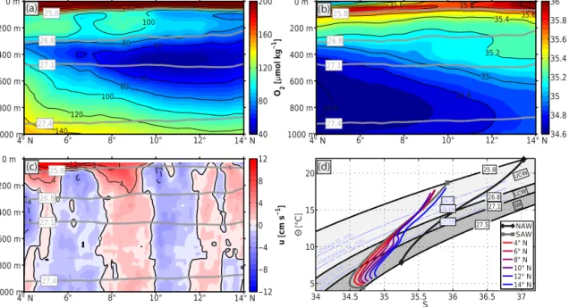
Figure 2.Mean sections of(a)oxygen,(b)salinity and(c)zonal velocity along 23^◦W between 4 and 14^◦N. Black contours denote isolines of the respective mean field. Gray solid contours mark mean surfaces of potential density in kg m⁻³. Note that no data of mean zonal velocity were derived for the upper 30 m.(d)Meanθ-Scharacteristics for North Atlantic Water (NAW) and South Atlantic Water (SAW) and for different latitudes along 23^◦W (details of reference regimes for NAW and SAW are given in the text). Data from about the upper 100 m of the water column were excluded. Black solid lines denote isopycnal surfaces, which define the different water mass regimes for UCW (upper central water), LCW (lower central water) and IW (intermediate water). Blue dashed lines denote isopycnal surfaces, which define different oxygen regimes with respect to the mean vertical oxygen profile in the ETNA.

2 Data and methods

This study uses a combined set of hydrographic, oxygen and velocity data, which consists of (i) repeat shipboard and moored observations, (ii) the MIMOC (monthly, isopycnal and mixed-layer ocean climatology), (iii) float observations provided by the Argo program and (iv) satellite derived sur- face velocities provided by Aviso. Further, data products of the different oxygen budget terms are used, which were de- rived in recent studies.

2.1 Repeat ship sections along 23^◦W

Hydrographic, oxygen and velocity data were obtained dur- ing repeated research cruises carried out mainly along 23^◦W in the ETNA in the period from 2006 to 2015 (1999 to 2015 for velocity; see Table 1 for details). The data set is an update of the 23^◦W ship section data used in Brandt et al. (2015). In the present study, data records from 4 to 14^◦N (ETNA OMZ regime) were taken into account.

Hydrographic and oxygen data were acquired during CTD (conductivity–temperature–depth) casts, typically performed on a uniform latitude grid with half-degree resolution. Ve- locity data were acquired with different Acoustic Doppler Current Profiler (ADCP) systems; vessel-mounted ADCPs (vm-ADCPs) recorded velocities continuously throughout

the section and pairs of lowered ADCPs (l-ADCPs), attached to the CTD rosette, recorded during CTD casts.

Based on these data sets, meridional sections of hydrogra- phy, oxygen and velocity were linearly interpolated for each ship section onto a homogeneous depth–latitude grid with a resolution of 10 m and 0.05^◦, respectively. Details of the methodology as well as on measurement errors are given in Brandt et al. (2010). For a single research cruise, the accu- racy of hydrographic and oxygen data was assumed to be generally better than 0.002^◦C, 0.002 and 2 µmol kg⁻¹ for temperature, salinity and dissolved oxygen, respectively. The accuracy of 1 h averaged velocity data from vm-ADCPs and single velocity profiles from l-ADCPs was better than 2–4 and 5 cm s⁻¹, respectively.

Mean sections along 23^◦W were calculated (Fig. 2a to c) from 13 (hydrography/oxygen) and 31 (velocity) individ- ual ship sections, respectively (Table 1). For the depth range 100–1000 m, the averaging of all sections yielded an average standard error of the mean fields (which is considered to re- sult mostly from oceanic variability) of about 1.8 µmol kg⁻¹, 0.06^◦C, 0.009 and 1.1 cm s⁻¹for oxygen, temperature, salin- ity and zonal velocity, respectively.

Moreover, a meridional section of the decadal oxygen and salinity trend was estimated. First, the data from each ship section were interpolated on a density grid (grid spacing 0.01 kg m⁻³)by applying an average depth–density relation

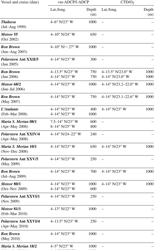
Table 1.Research cruises carried out in the eastern tropical North Atlantic between 4 and 14^◦N mainly along the 23^◦W section between 1999 and 2015. Different columns denote the latitude section along mean longitude (lat./long.) and maximum profile depth available/used here (depth in meters) for velocity observations performed with vessel-mounted and lowered Acoustic Doppler Current Profilers (vm-ADCPs/l- ADCPs) as well as for hydrographic and oxygen observations performed with a conductivity–temperature–depth sonde (CTD/O₂). Note that during some research cruises, two velocity and/or hydrographic sections were obtained.

Vessel and cruise (date) vm-ADCP/l-ADCP CTD/O₂

Lat./long. Depth Lat./long. Depth

(m) (m)

Thalassa (Jul–Aug 1999)

4–6^◦N/23^◦W 1000 – –

Meteor55 (Oct 2002)

4–10^◦N/24^◦W 650 – –

Ron Brown (Jun–Aug 2003)

4–10^◦N/∼27^◦W 1000 – –

PolarsternAnt XXII/5 (Jun 2005)

4–14^◦N/23^◦W 300 – –

Ron Brown 4–13.5^◦N/23^◦W 750 4–13.5^◦N/23.0^◦W 1000

(Jun 2006) 4–14^◦N/23^◦W 750 4–14^◦N/23.0^◦W 1000

Meteor68/2 (Jun–Jul 2006)

4–14^◦N/23^◦W 1000 4–14^◦N/23.2–22.0^◦W 1000 Ron Brown

(May 2007)

4–14^◦N/23^◦W 750 4–14^◦N/23.1–22.6^◦W 1000

L’Atalante 4–14^◦N/23^◦W 400 4–14^◦N/23^◦W 1000

(Feb–Mar 2008) 4–14^◦N/23^◦W 1000

Maria S. Merian08/1 7.5–14^◦N/23^◦W 600 – –

(Apr–May 2008) 8–14^◦N/25^◦W 800

PolarsternAnt XXIV/4 (Apr–May 2008)

4–14^◦N/24–22^◦W 240 – –

Maria S. Merian10/1 (Nov–Dec 2008)

4–14^◦N/23^◦W 650 4–14^◦N/23^◦W 1000 PolarsternAnt XXV/5

(May 2009)

4–14^◦N/23^◦W 250 – –

Ron Brown (Jul–Aug 2009)

4–14^◦N/23^◦W 700 4–14^◦N/23^◦W 1000 Meteor80/1 4–14^◦N/23^◦W 1000 4–14^◦N/23^◦W 1000

(Oct–Nov 2009) 4–14^◦N/23^◦W 600

PolarsternAnt XXVI/1 (Nov 2009)

4–14^◦N/23^◦W 250 – –

Meteor81/1 (Feb–Mar 2010)

4–13^◦N/22^◦W 1000 – –

PolarsternAnt XXVI/4 (Apr–May 2010)

4–13.5^◦N/23^◦W 250 – –

Ron Brown (May 2010)

4–14^◦N/23^◦W 1000 – –

Maria S. Merian18/2 4–5^◦N/23^◦W 1000 – –

(May–Jun 2011) 4–14^◦N/23^◦W 1000

Table 1.Continued.

Vessel and cruise (date) vm-ADCP/l-ADCP CTD/O₂ Lat./long. Depth Lat./long. Depth

(m) (m)

Maria S. Merian18/3 (Jun–Jul 2011)

4–14^◦N/23^◦W 600 4–14^◦N/23^◦W 1000 Ron Brown

(Jul–Aug 2011)

4–14^◦N/23^◦W 700 – –

Maria S. Merian22 4–8^◦N/23^◦W 1000 4–14^◦N/23^◦W 1000 (Oct–Nov 2012) 4–14^◦N/23^◦W 1000

Meteor106 (Apr–May 2014)

4–14^◦N/23^◦W 1000 4–14^◦N/23^◦W 1000 PolarsternPS88.2

(Nov 2014)

4–14^◦N/23^◦W 1000 4–14^◦N/23^◦W 1000 Meteor119

(Sep–Oct 2015)

4–14^◦N/23^◦W 1000 4–14^◦N/23^◦W 1000

in the depth range 0–1000 m. Then, linear regressions were calculated (using a 95 % confidence level to determine their significance) at each grid point in latitude–density space. The resulting sections were subsequently projected onto the depth grid.

In order to relate changes in oxygen to changes in salinity, shipboard observations were used to calculate the correlation between both variables at every grid point of the section. All calculations were evaluated in density space and the results were subsequently projected onto the depth grid.

2.2 Moored observations

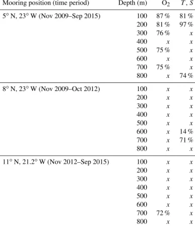
Multi-year moored observations (2009–2015) were per- formed in the ETNA to record hourly to interannual oxy- gen variability at three different positions: 5^◦N/23^◦W, 8^◦N/23^◦W and 11^◦N/21^◦W (see Table 2 for details about available data). All moorings were equipped with oxygen (AADI Aanderaa optodes of model types 3830 and 4330) and CTD sensors (Sea-Bird SBE37 microcats), which were attached next to each other on the mooring cable to allow an appropriate estimate of the dissolved oxygen on density surfaces. At every mooring site, eight evenly distributed op- tode/microcat combinations were installed in the depth range between 100 to 800 m, delivering multi-year oxygen time se- ries with a temporal resolution of up to 5 min.

Moorings were serviced and redeployed generally every 18 months. In order to achieve the highest possible long- term sensor accuracy, optodes and microcats were carefully calibrated against oxygen and CTD measurements (from a CTD/O₂ unit) by attaching them to the CTD rosette during regular CTD casts immediately prior to and after the mooring deployment period. Optodes were additionally calibrated in the laboratory on board to expand the range of reference cali-

bration points. Details of the optode calibration methodology are given in Hahn et al. (2014). The root mean square er- ror of temperature and salinity measurements (microcats) as well as dissolved oxygen measurements (optodes) was about 0.003^◦C, 0.006 and 3 µmol kg⁻¹, respectively.

Oxygen and salinity time series from the three mooring sites were 10-day low-pass filtered and subsequently inter- polated in depth space between 100 and 800 m. Based on this uniformly gridded data set, oxygen and salinity anoma- lies were calculated by (i) interpolating the moored and ship- board observations on a regular density grid (grid spacing 0.01 kg m⁻³), (ii) subtracting the respective mean profiles in density space obtained solely from shipboard observations and (iii) projecting the calculated anomalies back onto the depth grid (by applying an average depth–density relation).

This calculation removed the effect of isopycnal heave due to internal waves, mesoscale eddies or seasonal variability in the circulation. Depth averages of these oxygen and salinity anomaly time series were calculated for the two depth layers (200–400 and 500–800 m).

Linear trends were fitted to the oxygen and salinity anomaly time series from the combined observational data set of moored and shipboard observations for the two respec- tive depth layers. A weighted linear regression scheme was used, where a single ship section was weighted similar to 30 days of moored observations. Intervals on a 95 % confi- dence level were calculated for the estimated trends.

Moored observations were additionally used to calculate a correlation between oxygen and salinity (see also Sect. 2.1 for a similar analysis based on shipboard observations). As we consider only long-term variability, the correlation was computed from the 90-day median of the mooring time se- ries at the three respective latitudes. All calculations were

Table 2.Moored observations carried out in the eastern tropical North Atlantic between 2009 and 2015. Column “depth (m)” denotes the instrument depth at the respective mooring. Columns “O₂” and “T,S” denote the percentage of available oxygen and hydrographic data, respectively, compared to the total time period. A cross (“x”) marks data coverage of better than 99 %.

Mooring position (time period) Depth (m) O₂ T,S 5^◦N, 23^◦W (Nov 2009–Sep 2015) 100 87 % 81 % 200 81 % 97 %

300 76 % x

400 x x

500 75 % x

600 x x

700 75 % x

800 x 74 %

8^◦N, 23^◦W (Nov 2009–Oct 2012) 100 x x

200 x x

300 x x

400 x x

500 x x

600 x 14 %

700 x 71 %

800 x x

11^◦N, 21.2^◦W (Nov 2012–Sep 2015) 100 x x

200 x x

300 x x

400 x x

500 x x

600 x x

700 72 % x

800 x x

evaluated in density space and the results were subsequently projected onto the depth grid.

2.3 MIMOC

The monthly, isopycnal and mixed-layer ocean climatology (MIMOC) (Schmidtko et al., 2013) was used as a reference mean state in order to (i) perform a water mass analysis and (ii) quantify the temporal evolution of salinity anomalies in the tropical Atlantic. The climatological fields of potential temperature and salinity were interpolated on respective den- sity layers, and meanθ-Scharacteristics were defined for the two predominant water masses NAW and SAW found in the tropical Atlantic.

2.4 Argo float data set

All Argo data (Roemmich et al., 2009) avail- able for the study region were considered (https://doi.org/doi:10.13155/29825). Argo float data are collected and made freely available by the international Argo project and the national programs that contribute to it.

For the analysis, only delayed mode data with a data quality flag of “probably good” or better were used.

The Argo profile data were used in this study to quan- tify the temporal evolution of salinity anomalies in the tropi- cal Atlantic on two characteristic density surfaces (26.8 and 27.2 kg m⁻³). Anomalies of salinity were calculated with re- spect to the mean state given by MIMOC (see Sect. 2.3) for the period 2004–2016. Subsequently, mean salinity anoma- lies were calculated for different periods and a decadal ten- dency was estimated for the whole period.

2.5 Surface geostrophic velocity from altimeter products

Surface geostrophic velocities derived from satellite altime- try were used in this study to estimate the decadal change of the near-surface circulation and ventilation of the ETNA.

The altimeter product was produced by Ssalto/Duacs and dis- tributed by Aviso, with support from Cnes (http://www.aviso.

altimetry.fr/duacs/). Absolute geostrophic velocity data were taken from the delayed time global product MADT (Maps of Absolute Dynamic Topography) given in the version “all sat merged”. The data were extracted for the box 4–14^◦N/35–

20^◦W for the data period January 1993–September 2015 (processing date: 27 November 2015).

The two main variability patterns of the surface circula- tion in the tropical North Atlantic can be described by the first complex EOF (empirical orthogonal function) mode of the zonal geostrophic velocity anomaly, where the real part of the EOF pattern mimics the meridional migration of the NECC and the imaginary pattern reflects the variability in its strength (Hormann et al., 2012). We applied an EOF analy- sis to the grid-point-wise filtered (mean and seasonal cycle removed and subsequently 2-year low-pass filtered) time se- ries of Aviso zonal geostrophic velocity for the region given above in order to capture the interannual to decadal variabil- ity of the NECC/nNECC throughout the past decades. The first two EOF modes explained 23 and 14 % of the total vari- ance of the filtered time series and can be considered simi- larly to the real and imaginary patterns of the complex EOF as given in Hormann et al. (2012).

2.6 Oxygen budget terms

The oceanic oxygen distribution is governed on the one hand by oxygen-supplying processes such as physical transport and photosynthetic oxygen production and on the other hand by oxygen consumption driven by biological respiration and remineralisation of sinking organic matter (Karstensen et al., 2008; Brandt et al., 2015). In the ETNA, supply and consumption have not been in balance for the past decades (oxygen consumption was about 10–20 % larger than the supply processes), resulting in the aforementioned multi- decadal oxygen trend (Brandt et al., 2010; Hahn et al., 2014;

Karstensen et al., 2008). Mathematically, the oxygen bud- get is balanced when we allow for an oxygen tendency in addition to the oxygen supply and consumption terms.

However, in order to investigate causes for the change in the oxygen trend from decadal to multi-decadal timescales (Brandt et al., 2015), temporal changes in the oxygen bud- get terms have to be analyzed. Following Hahn et al. (2014) and Brandt et al. (2015), we formulate the non-steady-state depth-dependent oxygen budget for the ETNA over the lati- tude range 6–14^◦N as

[∂_tO₂

| {z }

[1]

]⁽ⁱ⁾=aOU R

| {z }

[2]

+K_e∂_yyO₂

| {z }

[3]

+K_ρ∂_zzO₂

| {z }

[4]

+ [R_O2

|{z}

[5]

]⁽ⁱ⁾, (1)

where the superscript on both sides of the equation denotes the time variation with respect either to the decadal(i=1) or multi-decadal (i=2)oxygen trend. The oxygen budget given by Eq. (1) describes the components contributing to the changes of the oxygen concentration, all of which are given in µmol kg⁻¹yr⁻¹. Term [1] (∂_tO₂)on the left-hand side of the equation marks the observed temporal change of oxygen (oxygen tendency). While the multi-decadal oxygen trend was already considered in Hahn et al. (2014), the es- timate of the decadal oxygen trend and its inclusion in the oxygen budget is a central part of this study (details of the calculation are given in Sect. 2.1). Term [2] (aOU R) de- fines the oxygen consumption, which has been determined

in Karstensen et al. (2008) following an approach that re- lates the apparent oxygen utilization (AOU) to water mass ages. Term [3] (K_e∂yyO₂) is the divergence of the merid- ional oxygen flux driven by eddy diffusion (Hahn et al., 2014). Term [4] (K_ρ∂_zzO₂)is the divergence of the diapy- cnal oxygen flux due to turbulent mixing (Fischer et al., 2013). Term [5] includes all other oxygen supply mecha- nisms which could not be directly estimated from observa- tional data: mean advection, zonal eddy diffusion and sub- mesoscale processes. This term is calculated as the residual oxygen supply based on terms [1] to [4]. Here, we follow the argumentation given in Hahn et al. (2014) by consider- ing the meridional structure of the eddy-driven meridional oxygen supply (term [3] in our Eq. 1) as well as the hori- zontal oxygen distribution (see also Fig. 10 therein); they ar- gued for a major contribution of the mean zonal advection in the upper 350 m, while zonal eddy diffusion and mean meridional advection have only a minor effect, and subme- soscale processes are not assumed to affect the oxygen dis- tribution well below the base of the mixed layer (Thomsen et al., 2016). Strictly, estimates of mean advection require the analysis of advective oxygen fluxes through the bound- aries of a closed volume. Such measurements are however not available. Nevertheless, in Sect. 4.3, we present a rough estimate of the zonal advective flux across the 23^◦W section derived from data taken only along that section. Note that vertical advection, which was recently proposed in a model study (Pena-Izquierdo et al., 2015) to be present as part of two stacked subtropical cells, is not considered in the ob- servationally based oxygen budget but will be discussed in Sect. 4.3 as well.

Given the data set in this study, a complete analysis of the temporal change of the consumption and supply terms, which ultimately are responsible for the change in the oxygen trend, cannot be performed due to insufficient data coverage and respective uncertainty reasons. Nevertheless, the decadal and multi-decadal oxygen trends ([∂_tO₂]⁽¹⁾and[∂_tO₂]⁽²⁾)are ap- plied separately in the oxygen budget. All other directly cal- culated terms (consumption, meridional eddy supply and di- apycnal supply) are kept time invariant, while the residual oxygen supply is calculated for the respective time periods (R_O⁽¹⁾

2 andR_O⁽²⁾

2)based on the two oxygen trends. This ad hoc approach is used to particularly discuss zonal advection as a potential driver for the change in the oxygen trend. However, in Sect. 4.3, we also analyze and discuss the potential of all other ventilation terms in having driven the decadal oxygen trend.

3 Results

In this section, results will be shown from the combined anal- ysis of moored, shipboard and float observations in the trop- ical Atlantic with a particular focus on the ETNA OMZ in order to investigate and quantify decadal changes of oxygen

2006 2008 2010 2012 2014 2016

−20 0 20

O2’ [µmol kg−1]

Year 2006 2008 2010 2012 2014 2016

−20 0 20

O2’ [µmol kg−1]

Year

2006 2008 2010 2012 2014 2016

−0.1 0 0.1

S’

Year 2006 2008 2010 2012 2014 2016

−0.1 0 0.1

S’

Year

(d) (c)

(b) (a)

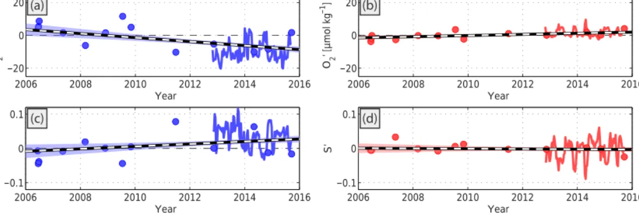
Figure 3. Oxygen (a and b) and salinity (c and d) anomaly time series from moored observations (solid line) at 11^◦N, 21^◦W and shipboard observations (dots) at 11^◦N, 23^◦W. Panels (a) and (c) show averages between 200 and 400 m. Panels (b) and (d) show averages between 500 and 800 m. Black dashed lines show respective trends from combined moored and shipboard observations:

(a)−12.2±4.9 µmol kg⁻¹decade⁻¹,(b)3.4±1.6 µmol kg⁻¹decade⁻¹,(c)0.036±0.026 decade⁻¹and(d)−0.004±0.018 decade⁻¹.

2006 2008 2010 2012 2014 2016

−20 0 20

O2’ [µmol kg−1]

Y ear 2006 2008 2010 2012 2014 2016

−20 0 20

O2’ [µmol kg−1]

Y ear

2006 2008 2010 2012 2014 2016

−0.1 0 0.1

S’

Y ear 2006 2008 2010 2012 2014 2016

−0.1 0 0.1

S’

Y ear

(d) (c)

(b) (a)

Figure 4. Oxygen (aand b) and salinity (candd) anomaly time series from moored (solid line) and shipboard (dots) observations at 8^◦N, 23^◦W. Panels (a)and (c)show averages between 200 and 400 m. Panels (b) and (d) show averages between 500 and 800 m.

Black dashed lines show respective trends from combined moored and shipboard observations: (a) −13.9±8.7 µmol kg⁻¹ decade⁻¹, (b)4.8±4.4 µmol kg⁻¹decade⁻¹,(c)−0.003±0.020 decade⁻¹and(d)−0.014±0.025 decade⁻¹.

as well as their correlation with changes in salinity. Changes in the velocity field were estimated based on repeat shipboard observations as well as satellite observations obtained mainly in the ETNA OMZ. Eventually, the oxygen budget of the ETNA was reanalyzed and revised from Hahn et al. (2014) with respect to both decadal and long-term oxygen changes.

3.1 Mean state in the ETNA

Given the mean 23^◦W section from shipboard observa- tions, the core of the deep OMZ is located at 10^◦N and at 430 m depth with a minimum oxygen concentration of 41.6 µmol kg⁻¹ (Fig. 2a). Between 100 and 250 m, pro- nounced oxygen maxima at 5^◦N and 8–9^◦N coincide well with the core positions of the near-surface NECC and nNECC (Fig. 2c). Similar patterns could not be observed in the salinity distribution (Fig. 2b). However, the largest merid- ional salinity gradient was found in the CW layer (25.8–

27.1 kg m⁻³)around 10^◦N and coincides with the northern edge of the near-surface eastward nNECC mirroring the tran- sition zone from SACW to NACW, i.e., from low salinity close to the Equator to high salinity in the northern part of the section.

The transition from SAW to NAW is well reflected in the θ-S diagram (Fig. 2d), which showsθ-S characteristics for particular latitudes based on the mean hydrographic ship sec- tion along 23^◦W (Fig. 2b; temperature not shown). Follow- ing Rhein et al. (2005), a simple water mass analysis was evaluated taking into account NAW and SAW, whose char- acteristics were defined from MIMOC for their respective source areas (25–30^◦N/60–10^◦W and 5^◦S–0^◦N/40^◦W–

0^◦E) (not shown). This revealed a strong spreading of SAW towards the north in the upper 300 m (UCW layer) with a SAW fraction of 0.9 close to the Cabo Verde archipelago at 13^◦N. Below 300 m (LCW and intermediate water (IW) lay- ers), fractions of SAW and NAW are similar, while NAW has

2006 2008 2010 2012 2014 2016

−20 0 20

O2’ [µmol kg−1]

Year 2006 2008 2010 2012 2014 2016

−20 0 20

O2’ [µmol kg−1]

Year

2006 2008 2010 2012 2014 2016

−0.1 0 0.1

S’

Year 2006 2008 2010 2012 2014 2016

−0.1 0 0.1

S’

Year

(d) (c)

(b) (a)

Figure 5. Oxygen (a and b) and salinity (c and d) anomaly time series from moored (solid line) and shipboard (dots) observa- tions at 5^◦N, 23^◦W. Panels (a)and (c)show averages between 200 and 400 m. Panels (b) and (d) show averages between 500 and 800 m. Black dashed lines show respective trends from combined moored and shipboard observations:(a)2.6±7.8 µmol kg⁻¹decade⁻¹, (b)−1.1±4.9 µmol kg⁻¹decade⁻¹,(c)−0.049±0.019 decade⁻¹and(d)−0.006±0.015 decade⁻¹.

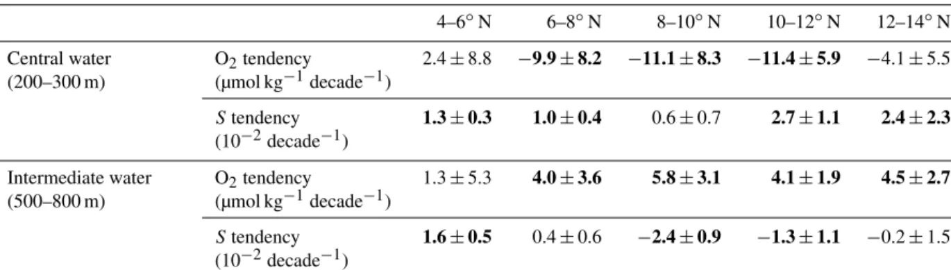
Table 3.Oxygen and salinity tendencies (2006–2015) with the 95 % confidence interval estimated for five different latitude boxes along 23^◦W and for the central water (200–300 m) and intermediate water (500–800 m) layers, respectively. Oxygen tendency was estimated from shipboard observations (cf. Fig. 6a) and salinity tendency was estimated from float observations (cf. Fig. 6c). Bold values define regimes with a significant decadal change.

4–6^◦N 6–8^◦N 8–10^◦N 10–12^◦N 12–14^◦N Central water

(200–300 m)

O₂tendency

(µmol kg⁻¹decade⁻¹)

2.4±8.8 −9.9±8.2 −11.1±8.3 −11.4±5.9 −4.1±5.5 Stendency

(10⁻²decade⁻¹)

1.3±0.3 1.0±0.4 0.6±0.7 2.7±1.1 2.4±2.3 Intermediate water

(500–800 m)

O₂tendency

(µmol kg⁻¹decade⁻¹)

1.3±5.3 4.0±3.6 5.8±3.1 4.1±1.9 4.5±2.7 Stendency

(10⁻²decade⁻¹)

1.6±0.5 0.4±0.6 −2.4±0.9 −1.3±1.1 −0.2±1.5

its southernmost extension at about 550 m with a fraction of 0.2 at 6^◦N.

3.2 Interannual variability and decadal change of oxygen and salinity

In this section, we present the temporal variability of oxygen and salinity obtained from shipboard, moored and float ob- servations of the most recent decade and investigate the cor- relation between these two variables. Decadal trends were derived at the aforementioned mooring positions as well as for the 23^◦W section between 4 and 14^◦N.

While the mean 23^◦W oxygen section shows a minimum oxygen concentration of 41.6 µmol kg⁻¹(see Sect. 3.1), in- dividual CTD profiles taken in the core of the deep OMZ between 300 and 700 m throughout the past decade regu- larly reached minimum oxygen concentrations well below 40 µmol kg⁻¹ (see also Stramma et al., 2009). An absolute minimum of 36.5 µmol kg⁻¹was observed at 12.5^◦N, 23^◦W

at 410 m during the RVMaria S. Meriancruise MSM22 in November 2012.

The combined analysis of shipboard and moored observa- tions (for details, see Sect. 2.2) revealed a remarkable oxy- gen change in the ETNA OMZ at latitudes 11 and 8^◦N throughout the past decade (Figs. 3a, b and 4a, b). Oxygen strongly decreased in the upper depth layer (200–400 m) and increased below (500–800 m), with salinity partly showing opposite trends (Figs. 3c, d and 4c, d). Superimposed on this decadal change, additional variability on intraseasonal to in- terannual timescales was observed. At 5^◦N, intraseasonal to interannual oxygen variability was the dominant signal (Fig. 5), and a decadal oxygen change could not be observed for this latitude. Note that besides the energetic salinity vari- ability on intraseasonal to interannual timescales, the combi- nation of shipboard and moored observations also suggests salinity fluctuations on a decade-long timescale in the upper depth layer (200–400 m; Fig. 5c).

Depth (m)

34.6 34.8

35.0 35.2

35.4 35.6

26.8

27.1 27.2

4° N 6° 8° 10° 12° 14° N

0

200

400

600

800

1000

Stendency[decade−1]

< −0.2

−0.1 0 0.1

> 0.2

95 % conf.< ≥

Depth (m) 34.8 35.0

35.2 35.4 35.6

26.8

27.1 27.2

4° N 6° 8° 10° 12° 14° N

0

200

400

600

800

1000

S tendency [decade−1]

< −0.2

−0.1 0 0.1

> 0.2

95 % conf.< ≥

Depth (m) 60

60 60

80

80

80

100 100

100

120 120

26.8

27.1 27.2

4° N 6° 8° 10° 12° 14° N

0

200

400

600

800

1000

O2 tendency [μmol kg−1 decade−1]

< −30

−20

−10 0 10 20

> 30

95 % conf.< ≥

(c) (b) (a)

Figure 6.Depth–latitude section of the linear trend (filled contours) of(a)oxygen and(b, c)salinity in the ETNA along 23^◦W. Pan- els(a)and(b)were calculated from repeat shipboard observations in the period 2006–2015. Panel(c)was calculated from Argo float observations in the period 2006–2015. All calculations were done on density surfaces with subsequent projection onto depth surfaces.

Gray-hatched areas mark non-significant regimes with respect to 95 % confidence. Mean fields of oxygen and salinity, respectively, are given as gray contours. Thick black contours define isopycnal surfaces 26.8, 27.1 and 27.2 kg m⁻³.

Based on shipboard observations, the 23^◦W section of decadal oxygen tendency for the period 2006–2015 (Fig. 6a) revealed coherent large-scale patterns of oxygen decrease and oxygen increase. Even though only a part of the lo- cal trends is statistically significant, the spatial coherence of the trends suggests robust trend patterns. Note also that significant patterns were larger than twice the smooth- ing and interpolation scale of the individual ship sections.

A strongly decreasing oxygen concentration with up to

−20 µmol kg⁻¹decade⁻¹ was found in the latitude range from 6 to 14^◦N and at a depth range 200 to 400 m (on average−5.9±3.5 µmol kg⁻¹decade⁻¹). Between 400 and 1000 m, oxygen was found to increase with an average mag- nitude of about 4.0±1.6 µmol kg⁻¹decade⁻¹between 6 and 14^◦N. Locally, a significant oxygen increase was observed

Figure 7.Vertical profiles of the slopes of the linear fits of oxygen against salinity with 95 % confidence intervals for moored (white- colored dashed line) and shipboard observations (colored dots) at positions(a)5^◦N, 23^◦W,(b)8^◦N, 23^◦W and(c)11^◦N, 21^◦W.

(d)Depth–latitude section (along 23^◦W) of the slope of the linear fit of oxygen against salinity (filled contours). Gray-hatched areas define non-significant regimes with respect to 95 % confidence.

below the OMZ core depth at 500–700 m in the latitude range 7–13^◦N as well as at 800–1000 m in the latitude range 4–

11^◦N. Box averages of decadal oxygen tendency for selected latitude and depth ranges together with their 95 % confidence estimates are presented in Table 3.

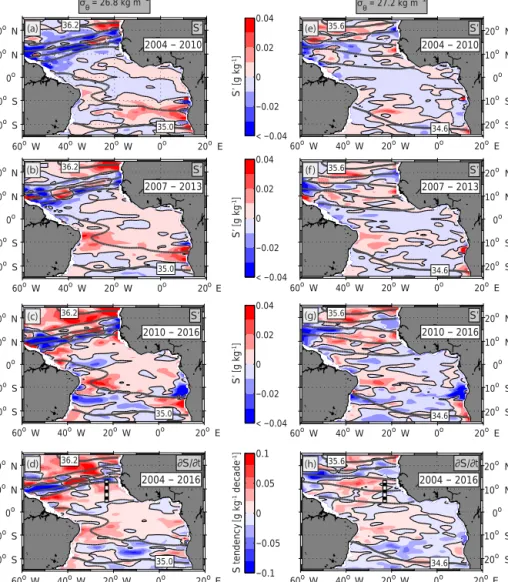
Shipboard observations mainly showed no significant decadal salinity tendency for the period 2006–2015 (Fig. 6b).

In a similar approach, we additionally calculated the decadal salinity tendency from Argo float observations (with refer- ence to the seasonal cycle of MIMOC) for the same time period (Fig. 6c). This resulted in a more robust estimate (see Table 3 for corresponding box averages) showing a salinity increase over almost the whole latitude range at the depth

60^oW 40^oW 20^oW 0^o 20^oE 20^o S 10^o S 0^o 10^o N 20^o N

34.6

35.6 ∂S/∂t

2004 − 2016 60^oW 40^oW 20^oW 0^o 20^oE

20^o S 10^o S 0^o 10^o N 20^o N

34.6

35.6 S’

2010 − 2016 60^oW 40^oW 20^oW 0^o 20^oE

20^o S 10^o S 0^o 10^o N 20^o N

34.6

35.6 S’

2007 − 2013 60^oW 40^oW 20^oW 0^o 20^oE

20^o S 10^o S 0^o 10^o N 20^o N

34.6

35.6 S’

2004 − 2010 σ_θ = 27.2 kg m⁻¹

−0.1

−0.05 0 0.05 0.1

Stendency[g kg-1 decade-1]

60^oW 40^oW 20^oW 0^o 20^oE 20^oS

10^oS 0^o 10^oN 20^oN

35.0

36.2 ∂S/∂t

2004 − 2016

< −0.04

−0.02 0 0.02 0.04

S’ [g kg-1]

60^oW 40^oW 20^oW 0^o 20^oE

20^oS 10^oS 0^o 10^oN 20^oN

35.0

36.2 S’

2010 − 2016

< −0.04

−0.02 0 0.02 0.04

S’ [g kg-1]

60^oW 40^oW 20^oW 0^o 20 E 20^oS

10^oS 0^o 10^oN 20^oN

35.0

36.2 S’

2007 − 2013

< −0.04

−0.02 0 0.02 0.04

S’ [g kg-1]

35.0 36.2

60^oW 40^oW 20^oW 0^o 20^oE 20^oS

10^oS 0^o 10^oN

20 N^o S’

2004 − 2010 σ_θ = 26.8 kg m⁻¹

(h) (g) (f) (e)

(d) (c) (b) (a)

o

Figure 8.Salinity anomalies (filled contours) in the tropical Atlantic at the isopycnal surface 26.8 kg m⁻³from Argo float observations for the period(a)2004–2010,(b)2007–2013 and(c)2010–2016.(d)Salinity trend (filled contours) calculated from all salinity anomalies at isopycnal surface 26.8 kg m⁻³between 2004 and 2016. The black–white dashed line marks the 23^◦W section between 4 and 14^◦N for reference. Gray contours in panels(a)to(d)define the mean salinity distribution. Panels(e)to(h)are same as(a)to(d)but for isopycnal surface 27.2 kg m⁻³.

range of about 100 to 350 m. Between 400 and 1000 m, salin- ity decreased between about 7 and 11^◦N as well as increased between about 4 and 7^◦N.

Variability in physical ventilation processes may drive co- herent changes in different tracers such as salinity or oxy- gen. Based on shipboard and moored observations, we cal- culated the correlation between oxygen and salinity (see Sect. 2.1 and 2.2 for details of the calculation) and iden- tified significant regimes along 23^◦W (Fig. 7). A signifi- cant negative correlation was found below the deep oxy- cline and south of the OMZ core (average slope∂O₂/∂S=

−255±140 µmol kg⁻¹)– a regime with a pronounced pos- itive gradient in salinity and negative gradient in oxygen on isopycnal surfaces in the northeast direction (cf. Fig. 2 in this study; Kirchner et al., 2009; Pena-Izquierdo et al., 2015).

North of the OMZ core, the correlation is positive, which agrees well with the positive oxygen and salinity gradient in northward direction in this regime. Note that above the deep oxycline (upper 300 m) the correlations obtained from moored and shipboard observations partly disagree with each other, which might be due to generally larger variability and the different time periods covered by both observational data sets.

The box averages (Table 3) for selected latitude and depth ranges show that significant decadal changes both in oxygen and salinity were found in the CW layer at 6–8^◦N and 10–

12^◦N as well as in the IW layer between 8 and 12^◦N. All significant tendencies were inversely related to each other and agreed well with regimes of significant anticorrelation of oxygen and salinity (Fig. 7).