Interannual to decadal changes in the western boundary circulation in the Atlantic at 11°S
Rebecca Hummels1, Peter Brandt1, Marcus Dengler1, Jürgen Fischer1, Moacyr Araujo2, Doris Veleda2, and Jonathan V. Durgadoo1
1GEOMAR Helmholtz Centre for Ocean Research Kiel, Kiel, Germany,2DOCEAN, Department of Oceanography, UFPE, Recife, Brazil
Abstract
The western boundary current system off Brazil is a key region for diagnosing variations of the Atlantic meridional overturning circulation (AMOC) and the southern subtropical cell. In July 2013 a mooring array was installed off the coast at 11°S similar to an array installed between 2000 and 2004 at the same location. Here we present results from two research cruises and thefirst 10.5 months of moored observations in comparison to the observations a decade ago. Average transports of the North Brazil Undercurrent and the Deep Western Boundary Current (DWBC) have not changed between the observational periods. DWBC eddies that are predicted to disappear with a weakening AMOC are still present. Upper layer changes in salinity and oxygen within the last decade are consistent with an increased Agulhas leakage, while at depths water mass changes are likely related to changes in the North Atlantic as well as tropical circulation changes.1. Introduction
The circulation system in the Atlantic transports large amounts of heat as part of the meridional overturning circulation (MOC) and is to a large extent responsible for the mean climate state in the Atlantic sector. On decadal to multidecadal time scales MOC variability plays a dominant role for climate variability in the entire Atlantic sector. Within the tropical Atlantic, interannual climate variability and associated rainfall variability have a multifaceted socioeconomic impact on the countries from adjacent continents.
The upper oceanflow at the western boundary at 11°S can be decomposed into contributions from the AMOC, the southern wind-driven subtropical cell (STC), and the Sverdrup-related transport [Schott et al., 2005]. Using a coupled climate model,Chang et al.[2008] showed that on decadal time scales a drastic (forced) slowdown of the Atlantic MOC (AMOC) reduces the strength and variability of the West African monsoon and hence the rainfall over West Africa. They identified significant changes in the ocean circulation responsible for their results: a slowdown of the AMOC leads to a reversal of the North Brazil Undercurrent (NBUC) and through interaction with the STCs, to a substantial warming of sea surface tempera- tures (SSTs) in the eastern and southern equatorial Atlantic. On shorter time scales such as interannual, the varia- bility of the tropical circulation including the NBUC is found to be mainly wind driven [Biastoch et al., 2008;Hüttl and Böning, 2006].
To date, the only time series of NBUC transport variability spanning several decades estimated from observations was presented inZhang et al.[2011]. In their study, where geostrophic NBUC transports were estimated from historical hydrographic observations, multidecadal variability has a range of about 6.7 Sverdrup (Sv, 106m3/s). Evidence for such strong NBUC variations from direct current observations is still pending.
In the framework of the German Bundesministerium für Bildung und Forschung project RACE, a mooring array consisting of four moorings equipped with current meters, was deployed in July 2013 at the western boundary at 11°S off the coast of Brazil. In addition, repeated shipboard observations along the sections at 11°S and 5°S were conducted. These observations repeat similar observations at the same location between 2000 and 2004. To address recent decadal changes, the present study compares the two distinct observational multiparameter time series data sets across the NBUC/Deep Western Boundary Current (DWBC) circulation system: the consistently reprocessed and studied 2000–2004 moored and ship measure- ments and the unpublished 2013–2014 analogue data set.
Geophysical Research Letters
RESEARCH LETTER
10.1002/2015GL065254
Key Points:
•Study of interannual to decadal variability of NBUC transports from observations and a model
•Transports over the period 2000–2004 and 2013–2014 have not changed significantly
•Water mass changes at the western boundary are related to Atlantic circulation changes
Supporting Information:
•Supporting Information S1
Correspondence to:
R. Hummels, rhummels@geomar.de
Citation:
Hummels, R., P. Brandt, M. Dengler, J. Fischer, M. Araujo, D. Veleda, and J. V. Durgadoo (2015), Interannual to decadal changes in the western boundary circulation in the Atlantic at 11°S,Geophys. Res. Lett.,42, 7615–7622, doi:10.1002/2015GL065254.
Received 16 JUL 2015 Accepted 20 AUG 2015
Accepted article online 25 AUG 2015 Published online 16 SEP 2015
©2015. American Geophysical Union.
All Rights Reserved.
2. Mean Flow
2.1. Ship Sections of Alongshore Velocity
Individual sections of alongshore velocity (slanted toward 36°T) for the available 7 ship cruises were con- structed from acoustic Doppler current profiler (ADCP) measurements between 2000 and 2014 (Figure 1a).
Shipboard ADCP data, covering the depth range between about 20 m and some intermediate depth (about 500–1000 m dependent on the instrument type used), were combined with data from ADCPs lowered on- station with the conductivity-temperature-depth (CTD) rosette in order to construct full-depth velocity sections (see Schott et al. [2005] for details). Transports are evaluated in density layers (indicated in Figures 1a–1c) defined by the following neutral density (γn) surfaces:γn= 24.5 kg m 3divides surface from thermocline waters, γn= 26.8 kg m 3 represents the lower limit of waters supplying the Equatorial Undercurrent. The boundary between intermediate and deep water was chosen asγn= 27.7 kg m 3. The North Atlantic Deep Water (NADW) layer is subdivided into upper, middle, and lower NADW using γn= 28.025 kg m 3andγn= 28.085 kg m 3.γn= 28.135 kg m 3is chosen as the border between NADW and Antarctic Bottom Water (AABW). The selection of these neutral density surfaces to distinguish the transport of different water masses follows Schott et al.[2005], but using neutral instead of potential density surfaces.
Neutral densities are the continuous analogue of discretely defined and locally referenced potential density sur- faces. They have a better accuracy infinding the best-practice isopycnal surface in the global ocean, and their calculation is simpler than the assembly of the discretely defined and referenced potential density surfaces [Jackett and McDougall, 1997].
The mean northward transport of the NBUC from the seven ship sections is 23 ± 3 Sv. Uncertainties are given in terms of the standard error. In the layers of the NADW the mean southward transport by the DWBC is 29 ± 7 Sv (Figure 1a). Compared toSchott et al.[2005], the averages are similar for the NBUC but somewhat lower for the DWBC based on thefivefirst cruises only (Table 1).
2.2. Mean Properties From the Moored Array
In the previous mooring data set (2000–2004) several mooring segments were lost due to instrument failure and requiredfilling of the gaps. For this study three gapfilling methods were tested and resulting transport time series are compared. For thefirst method, which was used inSchott et al.[2005], the four leading EOFs are calculated from the gappy mooring record (explaining 62% of the variance contained in mooring data) and subsequently used to reconstruct data tofill the gaps. The second method uses the four leading EOFs derived from the seven ship sections (explaining 86% of variance in shipboard data), which have a higher spatial, but lower temporal resolution. In another attempt multichannel singular-spectrum analysis (MSSA) is performed using the Singular Spectrum Analysis - MultiTaper Method toolkit described inGhil et al.
[2002] available under http://web.atmos.ucla.edu/tcd//ssa/. Using either of these three methods the gap- filled time series are low-passfiltered (cutoff at 10 days, as the focus here is on longer time scales) and subsequently mapped into sections every 2.5 days using a Gaussian-weighted interpolation with horizontal mapping scales of 20 km (cutoff radius at 150 km) and vertical mapping scales of 60 m (cutoff at 1500 m).
These sections are the base to obtain the transport time series (section 3).
Average transports calculated from the different gap-filled time series agree within 0.6 Sv for the NBUC and 0.1 Sv for the DWBC. Thus, in the following, the transport time series using the ship EOF gap-filling method is used. Average moored NBUC and DWBC transports for the two observational periods are not significantly different from each other (Table 1). The significance here and in the following is tested with thettest for com- parison of means at the 95% confidence interval. The average NBUC transport is 26 ± 1.1 Sv for the moored observations, which is also not significantly different from the ship-based estimate (Table 1). On the contrary, the average DWBC transport is only 17.5 ± 1.7 Sv, which is substantially lower than the ship-based estimate.
However, as shown below, the larger southward transport of the ship-based estimate is biased by intrasea- sonal variability (Figure 1e).
3. Transport Time Series
The transport time series from moored observations exhibits the transport variability of both NBUC and DWBC in much more detail (Figures 1d and 1e). NBUC transports mapped every 2.5 days range between about 10 and 45 Sv, DWBC transports between 60 Sv and 20 Sv. Twelve month averages of NBUC transports
Figure 1.(a) Individual velocity sections with transports estimated in the indicated boxes. (b) Average along shore velocity section from the seven ship sections shown in Figure 1a. (c) Average along shore velocity section from the moored observations. Red/black dashed lines in Figures 1a–1c enclose the boxes for NBUC/DWBC transport calculations. The insets in Figures 1b and 1c depict the orientation and location of the sections and moorings. Transport times series (d) for the NBUC and (e) for the DWBC estimated from moored observations (black line) together with the 90 day low-passfiltered time series (black dashed line). For the black lines data gaps arefilled with ship empirical orthogonal functions (EOFs), transport time series with data gapsfilled with EOFs from the mooring array as blue lines, and gapsfilled with the MSSA method as red lines. Red dots denote transports estimated from the shipboard observations.
for thefirst observational period (2000–2004) range between 25 ± 1.8 in March 2001 to February 2002 and 27.7 ± 3.1 Sv from March 2002 to February 2003 (Table 1). The average NBUC transport between July 2013 and May 2014 is 26.8 Sv ± 1.8 Sv. When considering the mean annual cycle from thefirst period, the transport in the later period (27.4 Sv) remains in the range of the 12 month averages of 2000–2004.
Within the NADW layer the moored transport time series does not show a decline in DWBC transport as could be interpreted from the ship sections. The 12 month averages range between 13 ± 3.9 and 21.4
± 2.8 Sv, whereas the estimate from the new observational period of 19.2 ± 5.2 Sv (Table 1) falls within this range ( 19.9 Sv when considering the annual cycle). As indicated in Figures 1a and 1e, four of the seven sections were conducted during elevated southwardflow well above the average. These sections captured the full extent of DWBC eddies and thus maxima in southward DWBC transport [Dengler et al., 2004;Schott et al., 2005].
To contextualize the observed interannual transport time series of the NBUC, it is compared to other available transport estimates (Figure 2). Outputs from the hindcast simulation of a 1/10° global nested ocean model, INALT01 [Durgadoo et al., 2013], covering the time period between 1956 and 2007 are analyzed. Detailed analysis of the model runs at 11°S shows that transports calculated in a predefined box (as used for the observa- tions) and from the coast to thefixed longitude of 33°W (see Figure S1 in the supporting information for details) are significantly correlated (r= 0.89) at the 95% confidence level using attest for correlation. This permits the direct comparison of the box transports from observations (Table 1) with trans- ports from the numerical simulations until 33°W.
Interannual variability between the INALT01 simulation and transport esti- mates from observations agrees well for the period 2000 to 2004 (Figure 2), e.g., even the increased annual mean transport in 2003 is reproduced by the model. As a measure of the strength of interannual variability, the standard deviation (std) of the 15 year high- pass-filtered transport time series from INALT01 is similar to that of the annual mean observed transports, 1.38 Sv and 1.3 Sv, respectively.
The agreement on interannual time scale encouraged us to further compare decadal variability of INALT01 trans- ports to the geostrophic transport Figure 2.Annual transport anomaly time series calculated for INALT01
(magenta) until 33°W, together with geostrophic transport anomalies fromZhang et al.[2011] (blue) and annual transport anomalies from the moored observations (black squares) calculated within the red dashed box as indicated in Figure 1c. The long-term variability (15 year low-pass filtered) is illustrated by dashed lines according to the color coding.
Anomalies of the different time series are calculated with respect to the mean of the INALT01 simulation for overlapping periods; i.e., subtracted means are 16.25 Sv forZhang et al.[2011], 14.88 Sv for INALT01, and 25.2 Sv for moored observations.
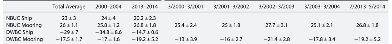
Table 1. Average Transports Estimated From Shipboard and Moored Observations (Gaps Filled With Four Leading EOFs Calculated From the Ship Sections) in Different Time Periodsa
Average Transport Estimates (Sv) Annual Transport Estimates (Sv)
Total Average 2000–2004 2013–2014 3/2000–3/2001 3/2001–3/2002 3/2002–3/2003 3/2003–3/2004 7/2013–5/2014
NBUC Ship 23 ± 3 24 ± 4 20.2 ± 2.3
NBUC Mooring 26 ± 1.1 25.8 ± 1.2 26.8 ± 1.8 25.4 ± 2.4 25 ± 1.8 27.7 ± 3.1 25.1 ± 2.1 26.8 ± 1.8
DWBC Ship 29 ± 7 34.8 ± 8.6 14.7 ± 0.6
DWBC Mooring 17.5 ± 1.7 17 ± 1.6 19.2 ± 5.2 13 ± 3.9 16 ± 2.7 21.4 ± 2.8 17.8 ± 3.4 19.2 ± 5.2
aAverages are calculated as the mean of the individual transport estimates, and error estimates are standard errors. The number of degrees of freedom (n) for the calculation of the standard error for the ship sections is taken as the number of individual sections; for the time series it is the length of the time series divided by the decorrelation time scale of the autocorrelation, i.e., ~50 days.
calculations presented inZhang et al.[2011]. However,Zhang et al.[2011] included data from 12°S to 4.5°S and between the coast and 33°W–28°W. As the model also shows significant correlation and similar interann- ual variability between transport time series at 11°S and 5°S (r= 0.62, std5°S= 1.55 Sv) the comparison of all of these transport time series is appropriate.
The phase and period (~30 years) of the multidecadal NBUC variability agree among the model and the study ofZhang et al.[2011]. However, the range of multidecadal variability obtained byZhang et al.[2011] when considering data between 12°S and 4.5°S (Figure S2) is ~6.7 Sv and thus larger compared to the range derived for INALT01 at 5°S (~5.5 Sv) and 11°S (~4.6 Sv). Furthermore, the larger multidecadal variability at 5°S compared to 11°S for INALT01 points toward local forcing mechanisms. The role of wind-driven versus thermohaline forcing for NBUC variability is being explored in a separate study.
4. Decadal Changes in Salinity and Oxygen
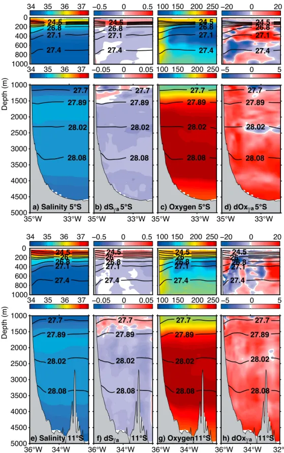
Comparison of the average sections of salinity and oxygen for the period of 2000–2004 (five cruises for salinity and four for oxygen) and 2013–2014 (two cruises) gives an indication of decadal changes in the water mass properties at this location. Here the focus is on water mass changes on isopycnal coordinates, the robustness of the observed trends, and possible causes. Therefore, salinity and oxygen differences on isopycnal coordinates between the two observational periods are examined for two latitudes, 5°S and 11°S (Figure 3). To further corroborate the detected trends in salinity, the hydrographic data from the seven ship sections are complemented by hydrographic data from the World Ocean Atlas, the Argo program, and CTD data from cruises carried out by the Brazilian Navy (Figures S4 and S5).
4.1. Salinity
In general, the decadal changes in salinity are coherent between 5°S and 11°S (Figures 3b and 3f) and indi- cate an increase within the central water range aboveγn= 26.8 kg m 3(Figures 3a and 3e). Within the Antarctic Intermediate Water (AAIW) layer the difference of the two observational periods shows only small trends with a slight decrease in the upper part of that layer changing toward an increase in salinity at the border to the NADW (γn= 27.7 kg m 3). However, evaluation of historical hydrographic data shows an increase in salinity (even if reduced in magnitude to the trend in the central water range) throughout the AAIW range (Figures S4b and S5). Hence, the results concerning the AAIW appear ambiguous, while the increase in salinity aboveγn= 26.8 kg m 3 is consistent among the ship sections and the historical hydrographic data (Figures 3 and S4a). Within the depth layers associated with the NADW, salinity gener- ally decreases. The trends below 1500 m obtained exclusively from the seven ship sections analyzed in this study (no additional data available) are small in magnitude but different from zero according to the errors of the trend (Figure S4b).
4.2. Oxygen
Within the central and intermediate water range decadal oxygen changes are noisy (Figures 3 and S5b). The coherent features between 5°S and 11°S in the upper layer are the general patchiness and a decrease in oxy- gen within the AAIW layer between 600 and 1000 m close to the western boundary (aroundγn= 27.4 kg m 3).
At depths of the NADW the oxygen signal is coherent with depth and among 5°S and 11°S showing an increase in oxygen during the last decade (Figures 3d and 3h).
5. Summary and Discussion
The variability in NBUC and DWBC transport at 5°S and 11°S in the Atlantic is investigated using seven ship cruises, two mooring time series (2000–2004 and 2013–2014), and a numerical simulation. While former studies relying on direct observations focused more on intraseasonal to interannual variability of transports and velocity [Dengler et al., 2004;Schott et al., 2005;Veleda et al., 2012], the focus of this study is on interannual to decadal changes in transports, velocity, salinity, and oxygen at this location.
Transport estimates from the ship surveys as well as from the moored observations show that the NBUC transport is similar in magnitude and variability in 2013–2014 compared to the period 2000–2004 (Figure 1 and Table 1). Interannual NBUC transport variability based on direct velocity observations agrees with the interannual variability obtained from the forced ocean model simulation (Figure 2).
Figure 3.(a, e) Mean salinity and (c, g) oxygen (inμmol kg 1) sections at 5°S (top row) and 11°S (bottom row) for the seven cruises averaged on density surfaces and converted back to pressure coordinates as well as (b, f) salinity and (d, h) oxygen (inμmol kg 1) differences between the two observational periods (2013–2014 and 2000–2004) calculated on density surfaces and subsequently converted back to the pressure grid. In each panel contoured density surfaces areγn= [24.5, 25, 25.5, 26, 26.3, 26.8, 27.1 27.4, 27.7, 27.89, 28.02, 28.08] kg m 3as also shown in Figures S4 and S5.
The error estimates of NBUC transports obtained from moored observations suggest that decadal varia- bility operating with an amplitude of≥2.5 Sv (as found byZhang et al.[2011] and the numerical simula- tion) would be identifiable with the current observing system at 11°S but could not be detected so far.
The observations further show that the transport in the NADW layer at 11°S is still (in 2013–2014) accomplished by deep eddies, which have similar properties as assessed during the period of 2000–2004 (Figure S3). In this layer average transports also do not exhibit significant changes in 2013–2014 compared to the period of 2000–2004 (Table 1).Dengler et al.[2004] suggested a laminarflow at 11°S instead of deep eddies for a weaker DWBC, which is obviously not the case yet.
Increasing salinity over the past decades within the NBUC region was reported byBiastoch et al.[2009] asso- ciated with an increase of Agulhas leakage due to the strengthening of the westerlies [Durgadoo et al., 2013].
The Agulhas leakage constitutes the main source of heat and salt for the surface branch of the AMOC.
Biastoch et al.[2009] obtained a salinity trend of +0.028/decade between 1965 and 2005 from available observational data between 100 and 600 m depth and between 40°W–30°W and 5°S–10°S. The salinity change on isopycnals presented in this study averaged over the entire section and between 100 and 600 m depths results in a salinity increase of 0.024 at 11°S between the two observational periods, which are roughly a decade apart. However, the ship sections as well as the analysis of additional hydrographic data show that the strongest salinity trend above 0.1/decade is found in the neutral density range 25.0 kg m 3≤γn≤26.8 kg m 3between about 100 und 250 m depth (Figures 3, S4, and S5).
Apart from these trends, interannual variability of salinity is most pronounced in this density range (Figure S4), where amplitudes above 0.1 were observed. Recently,Kolodziejczyk et al.[2014] could indeed track salinity anomalies from the Agulhas region toward the NBUC region propagating along the northward and westward branch of the subtropical gyre of the South Atlantic. They report salinity anomalies of up to +0.12 reaching the western boundary in 2013 on the isopycnalγn= 26.3 kg m 3consistent with this study (Figures 3, S4, and S5).
Within the upper AAIW layer, salinity changes on isopycnals appear ambiguous between the ship sections and the analysis of historical hydrographic data (Figures 3 and S4). In addition, decadal oxygen changes within this layer are patchy (Figures 3d and 3h). Within the depth range of the AAIW and within the longitudinal range, where a southward recirculation of the NBUC was identified [Schott et al., 2005;Silva et al., 2009, Figure 1], ele- vated eddy kinetic energy was detected in previous observations [Boebel et al., 1999]. This elevated mesoscale variability (see also Figures S1b–S1d) together with the large lateral gradients in the mean oxygen distribution (Figures 3c and 3g) might be responsible for the patchiness in the oxygen trends in this region.
The most coherent feature within the AAIW layer between 5°S and 11°S is the oxygen decrease between 600 and 1000 m close to the western boundary, where northward velocities are strongest. A possible explanation of the observed decrease here is an increased Agulhas leakage. Oxygen concentrations on neutral density surfaceγn= 27.4 kg m 3are higher in the South Atlantic compared to the South Indian Ocean (Figure S6).
At the transition from AAIW to NADW (γn= 27.7 kg m 3) an increase in salinity is observed, whichfits to the generalfindings of changes in the AAIW layer: a warming and increase in salinity on isopycnals denser than the AAIW salinity minimum and usually a cooling and freshening on lighter isopycnals [Schmidtko and Johnson, 2012].
In summary, the salinity increase within the central water and the oxygen decrease within the AAIW range supportfindings from previous studies suggesting an increased Agulhas leakage. Ambiguous salinity trends and a patchiness of oxygen trends within the upper AAIW layer point toward the existence of strong mesoscale activity.
Within the NADW range salinity changes on isopycnals averaged between 1500 and 4000 m over the entire section at 11°S result in a freshening of 0.007/decade. Regarding the middle and lower NADW, this is in gen- eral agreement with the results ofDickson et al.[2002], who reported a freshening trend of 0.01/decade over the last 3–4 decades in the deep and abyssal layers of the Labrador Sea. They attribute this freshening to the general freshening of the dense overflows farther upstream instead of local climate forcing, which now seems detectable south of the equator. However, this does not explain the oxygen increase within this layer.
Steinfeldt and Rhein[2004] suggested that the decrease in the fraction of“young”NADW between 1999 and 2002 was linked to an enhanced recirculation of the DWBC close to the equator. Consequently, it could be speculated that if this recirculation has decreased within recent years and NADW follows a more direct route
along the western boundary, oxygen should be less detrained, and hence, a positive oxygen trend would be expected as detected at 5°S and 11°S (Figures 3d and 3h). Unfortunately, no observations exist to support this hypothesis. Changes in the upper NADW could mark the arrival of low salinity and increased oxygen waters formed during the intense convection period in the late 80s and early 90s in the subpolar North Atlantic [Molinari et al., 1998;van Sebille et al., 2011]. In a recent study,Rhein et al.[2015] estimate a travel time of newly formed NADW from the subpolar latitudes to 10°S of about 27 years. This time scale would support the above hypothesis explaining the observed salinity and oxygen trends. However, such travel time estimates are subject to large uncertainties and mixing along the DWBC route with ambient water masses could dominate the signal arriving at 10°S.
This study gives afirst insight from moored and shipboard observations into interannual to decadal changes within the western boundary circulation system within the tropical South Atlantic, which is a key region in order to understand interannual to decadal AMOC and STC variability. The mooring time series at 11°S, which is anticipated to continue, represents a contribution to the South AMOC observing system [Meinen et al., 2013], which still needs to be further developed compared to its North Atlantic counterpart to allow assessing interannual to decadal AMOC variability, its latitudinal coherence, and its impact on climate variations in the tropics and beyond.
References
Biastoch, A., C. W. Böning, J. Getzlaff, J.-M. Molines, and G. Madec (2008), Causes of interannual-decadal variability in the meridional overturning circulation of the midlatitude North Atlantic Ocean,J. Clim.,21(24), 6599–6615.
Biastoch, A., C. W. Boning, F. U. Schwarzkopf, and J. R. E. Lutjeharms (2009), Increase in Agulhas leakage due to poleward shift of Southern Hemisphere westerlies,Nature,462(7272), 495–498.
Boebel, O., C. Schmid, and W. Zenk (1999), Kinematic elements of Antarctic Intermediate Water in the western South Atlantic,Deep Sea Res.
Part II,46(1–2), 355–392.
Chang, P., R. Zhang, W. Hazeleger, C. Wen, X. Wan, L. Ji, R. J. Haarsma, W.-P. Breugem, and H. Seidel (2008), Oceanic link between abrupt changes in the North Atlantic Ocean and the African monsoon,Nat. Geosci.,1(7), 444–448.
Dengler, M., F. A. Schott, C. Eden, P. Brandt, J. Fischer, and R. J. Zantopp (2004), Break-up of the Atlantic deep western boundary current into eddies at 8 degrees S,Nature,432(7020), 1018–1020.
Dickson, B., I. Yashayaev, J. Meincke, B. Turrell, S. Dye, and J. Holfort (2002), Rapid freshening of the deep North Atlantic Ocean over the past four decades,Nature,416(6883), 832–837.
Durgadoo, J. V., B. R. Loveday, C. J. C. Reason, P. Penven, and A. Biastoch (2013), Agulhas leakage predominantly responds to the Southern Hemisphere westerlies,J. Phys. Oceanogr.,43(10), 2113–2131.
Ghil, M., et al. (2002), Advanced spectral methods for climatic time series,Rev. Geophys.,40(1), 1003, doi:10.1029/2000RG000092.
Hüttl, S., and C. W. Böning (2006), Mechanisms of decadal variability in the shallow subtropical-tropical circulation of the Atlantic Ocean: A model study,J. Geophys. Res.,111, C07011, doi:10.1029/2005JC003414.
Jackett, D. R., and T. J. McDougall (1997), A neutral density variable for the world’s oceans,J. Phys. Oceanogr.,27(2), 237–263.
Kolodziejczyk, N., G. Reverdin, F. Gaillard, and A. Lazar (2014), Low-frequency thermohaline variability in the Subtropical South Atlantic pycnocline during 2002–2013,Geophys. Res. Lett.,41, 6468–6475, doi:10.1002/2014GL061160.
Meinen, C. S., S. Speich, R. C. Perez, S. Dong, A. R. Piola, S. L. Garzoli, M. O. Baringer, S. Gladyshev, and E. J. D. Campos (2013), Temporal variability of the meridional overturning circulation at 34.5°S: Results from two pilot boundary arrays in the South Atlantic,J. Geophys. Res.
Oceans,118, 6461–6478, doi:10.1002/2013JC009228.
Molinari, R. L., R. A. Fine, W. D. Wilson, R. G. Curry, J. Abell, and M. S. McCartney (1998), The arrival of recently formed Labrador sea water in the Deep Western Boundary Current at 26.5°N,Geophys. Res. Lett.,25(13), 2249–2252, doi:10.1029/98GL01853.
Rhein, M., D. Kieke, and R. Steinfeldt (2015), Advection of North Atlantic Deep Water from the Labrador Sea to the southern hemisphere, J. Geophys. Res. Oceans,120, 2471–2487, doi:10.1002/2014JC010605.
Schmidtko, S., and G. C. Johnson (2012), Multidecadal warming and shoaling of Antarctic Intermediate Water,J. Clim.,25(1), 207–221.
Schott, F. A., M. Dengler, R. Zantopp, L. Stramma, J. Fischer, and P. Brandt (2005), The shallow and deep western boundary circulation of the South Atlantic at 5 degrees–11 degrees S,J. Phys. Oceanogr.,35(11), 2031–2053.
Silva, M., M. Araujo, J. Servain, P. Penven, and C. A. D. Lentini (2009), High-resolution regional ocean dynamics simulation in the southwestern tropical Atlantic,Ocean Model.,30, 256–269.
Steinfeldt, R., and M. Rhein (2004), Spreading velocities and dilution of North Atlantic Deep Water in the tropical Atlantic based on CFC time series,J. Geophys. Res.,109, C03046, doi:10.1029/2003JC002050.
van Sebille, E., M. O. Baringer, W. E. Johns, C. S. Meinen, L. M. Beal, M. F. de Jong, and H. M. van Aken (2011), Propagation pathways of classical Labrador Sea water from its source region to 26°N,J. Geophys. Res.,116, C12027, doi:10.1029/2011JC007171.
Veleda, D., M. Araujo, R. Zantopp, and R. Montagne (2012), Intraseasonal variability of the North Brazil Undercurrent forced by remote winds, J. Geophys. Res.,117, C11024, doi:10.1029/2012JC008392.
Zhang, D., R. Msadek, M. J. McPhaden, and T. Delworth (2011), Multidecadal variability of the North Brazil Current and its connection to the Atlantic meridional overturning circulation,J. Geophys. Res.,116, C04012, doi:10.1029/2010JC006812.
Acknowledgments
This study was funded by the Deutsche Bundesministerium für Bildung und Forschung (BMBF) as part of the pro- jects RACE (03F0651B) and SPACES (03G0835A) and through support of R/V Sonnecruises and by the Deutsche Forschungsgemeinschaft as part of the project FOR1740 and through cruises with R/VMeteor. The INALT01 model experiments were performed at the high-performance computing centers in Stuttgart (HLRS) and at the Christian- Albrechts-Universität zu Kiel (NESH). The authors are grateful for continuing sup- port from GEOMAR Helmholtz Centre for Ocean Research Kiel and thank the Brazilian Navy for making their hydro- graphic data available. Argo data were collected and made freely available by the International Argo Project and the national initiatives that contribute to it (http://www.argo.net). Data from the World Ocean Atlas Database were retrieved from https://www.nodc.noaa.
gov/OC5/woa13/woa13data.html. We would like to thank C. Böning and A.
Köhl for their helpful discussions and two anonymous reviewers for their comments that lead to significant improvements of the manuscript.
The Editor thanks two anonymous reviewers for their assistance in evaluating this paper.